GRASP and Iterated Local Search-Based Cellular Processing algorithm for Precedence-Constraint Task List Scheduling on Heterogeneous Systems

Abstract

High-Performance Computing systems rely on the software’s capability to be highly parallelized in individual computing tasks. However, even with a high parallelization level, poor scheduling can lead to long runtimes; this scheduling is in itself an NP-hard problem. Therefore, it is our interest to use a heuristic approach, particularly Cellular Processing Algorithms (CPA), which is a novel metaheuristic framework for optimization. This framework has its foundation in exploring the search space by multiple Processing Cells that communicate to exploit the search and in the individual stagnation detection mechanism in the Processing Cells. In this paper, we proposed using a Greedy Randomized Adaptive Search Procedure (GRASP) to look for promising task execution orders; later, a CPA formed with Iterated Local Search (ILS) Processing Cells is used for the optimization. We assess our approach with a high-performance ILS state-of-the-art approach. Experimental results show that the CPA outperforms the previous ILS in real applications and synthetic instances.

1. Introduction

According to the website www.top500.org, the supercomputer Fugaku from the Fujitsu RIKEN Center for Computational Science in Japan consists of 7,299,072 processing units. The above gives an outstanding parallel computing power. However, without accurate and efficient scheduling methods, parallel programs can be very computationally inefficient. In this paper, we approach the precedence-constraint task scheduling of parallel programs on systems formed by heterogeneous processing units to minimize the final computing time [1]. Scheduling is a well-known NP-hard optimization problem [2], as well as the task scheduling for parallel systems [3]. Therefore, different scheduling approaches were developed for this problem: Heuristics [4,5,6,7], Local Searches [8,9,10], and Metaheuristics [11,12,13,14,15]. Unfortunately, the wide variety of works in the state-of-the-art differs in their objective definitions and uses different sets of instances. From the relevant works in the state-of-the-art, we highlight [11]. To our knowledge, it is the only work that compares the obtained results against the optimal values for their synthetic instances, which are fourteen scheduling problem instances that are easily reproducible. In [11], four high-performance Iterated Local Search (ILS) algorithms are proposed, the best ILS nearly reaches all the optimal values, obtaining an approximation factor of 1.018 (desirable values are near to 1.0). Thus, we assess our proposal with the best-proposed algorithm in [11].

Scheduling precedence-constraint tasks for heterogeneous systems has been addressed with a lot of variants: energy-aware [16], idle energy-aware [8,17], energy constraint [18], communication delays and energy [19], budget constraint [20], fault-tolerant [21], security-aware [22], volunteer computing systems [23], among others. A related problem is the job shop problem [24]. However, in a parallel program, scheduling is a single job (the parallel program) without dedicated machines to a single task. On the other hand, in scheduling, any machine can compute any task, similar to the job shop’s flexible problem [25] but with a single job. In Section 2, we detail our studied version of scheduling precedence-constraint tasks on heterogeneous systems.

In this paper, we use a recent metaheuristic optimization framework called Cellular Processing Algorithm (CPA) [26,27]. CPAs are more like a framework than a strict algorithm. The main idea is to cycle between exploring the search space with multiple limited-effort algorithms (Processing Cells) and sharing information (communication) among these Processing Cells. The limited-effort algorithms can explore the search space independently from one another and communicate their findings using shared memory or other combining methods. However, despite the communication, the Processing Cells should keep looking independently and not as a whole algorithm. In this way, we avoid the computational cost of converging the whole population (when the solutions reach the same search space area) or exploring the search space with a single solution algorithm (like Greedy Randomized Adaptive Search Procedure (GRASP) or Iterated Local Search).

As stated before, CPAs are flexible, e.g., a cellular processing algorithm can initialize each Processing Cell with different heuristics to ensure the splitting of the search space among the Processing Cells [28]. Additionally, the Processing Cells can be homogeneous or heterogeneous, which means that the Processing Cells can be multiple instances of the same algorithm [29] or completely different algorithms [30]. Furthermore, we can create a soft-heterogeneous CPA with differently-configured instances of the same algorithm. Thus, with all its flexibility, there is still much to research for CPAs and its applications.

The remainder of the paper is organized as follows. Section 2 details the studied precedence-constraint task scheduling problem on heterogeneous systems. In Section 3, we introduce the related and proposed algorithms for our experimentation. Section 4 contains the experimental setup, and parameter settings. Section 5 analyzes the experimental results according to the achieved median values using non-parametric statistical tests. Finally, Section 6 gives our conclusions and future work on scheduling precedence-constraint tasks on heterogeneous systems and the Cellular Processing Algorithms.

2. Problem Description

The High-Performance Computing systems (HPC) addressed in this paper consist of a set of heterogeneous machines M completely interconnected. Every machine $m_j\in M$ has different hardware characteristics, which yields different processing times for the same task. Without loss of generality, we make the following assumptions:

• Every machine has a connection link with any other machine.
• The communication links have no conflicts.
• All the communication links operate at the same speed.
• Every machine can send/receive information to/from another while executing a task.
• The communication cost between tasks in the same machine is depreciated.

2.1. Instance of the Problem

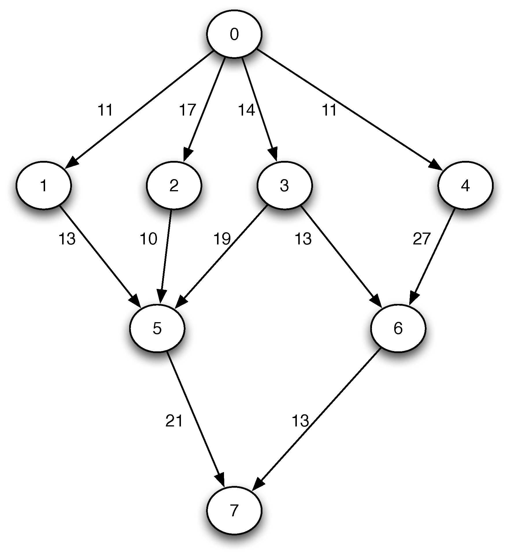
An instance of the problem is made up of two parts, a Directed Acyclic Graph (DAG) and the computation cost of the tasks in every machine. We represent the set of tasks of a parallel computing program and their precedencies as a DAG. Therefore, the parallel program is represented as the graph $G=(T,C)$ where T is the set of tasks (vertices) and C is the set of communication costs between tasks (edges) (see Figure 1). The complete instance of the problem is formed by G and the computational costs $P_{i,j}$ of each task $t_i$ in every machine $m_j$ (see

Table 1. Computational costs of the tasks $P_{i,j}$ on every machine.

Task	${\mathit{m}}_1$	${\mathit{m}}_2$	${\mathit{m}}_3$
$t_0$	11	13	9
$t_1$	10	15	11
$t_2$	9	12	14
$t_3$	12	16	10
$t_4$	15	11	19
$t_5$	13	9	5
$t_6$	11	15	13
$t_7$	11	15	10

).

Any task $t_i$ cannot be initiated until its precedent tasks $t_j\in T|(t_j,t_i)\in C$ finalize their executions and communications $\left(C_{j,i}\right)$. However, when any pair of tasks are scheduled in the same machine, the actual communication cost $C_{j,i}^{\prime }$ between them is depreciated.

2.2. Objective Function

In this work, we follow the approach of list scheduling algorithms. List scheduling algorithms are a family of heuristics in which tasks are ordered according to a particular priority criterion. The task execution order is equivalent to a DAG $G=(T,C)$ topological order from the task graph, without violating the precedence constraints.

Table 2. Tasks’ order of execution.

Task

${\mathit{t}}_0$

${\mathit{t}}_4$

${\mathit{t}}_3$

${\mathit{t}}_1$

${\mathit{t}}_2$

${\mathit{t}}_5$

${\mathit{t}}_6$

${\mathit{t}}_7$

shows an example of a feasible order for the task graph from Figure 1.

Although the task order of execution is not indispensable for the scheduling, it simplifies the objective function computation [1], i.e., because it is not necessary to compute different combinations of the tasks, starting and finish times, to compute the minimum makespan [3,15,17]. However, this approach has the deficiency that the optimal value may not be possible in every task execution order. Algorithm 1 details the computation of the makespan objective function, using the computation times $P_{i,j}$ from Table 1 and a time counter ($Tim{e}_j$) for each machine, to keep track of the last executed task in each machine.

Algorithm 1 Makespan objective function

Input: $G=(T,C)$, computational costs $P_{t_i,j}$, and an order execution of the tasks $O=\{o_1,\cdots ,o_{\left|T\right|}\}$.

Output: $makespan$

1: $Tim{e}_j\leftarrow 0$, $\forall m_j\in M$

2: for $x=1$ to $\left|O\right|$ do

3:   $t_{current}$ = $o_x$

4:   $j\leftarrow$ the index of the machine $m_j$ assign to $t_{current}$

5:   if $\forall u=\{1,...,|T\left|\right\}\nexists (t_u,t_{current})\in C$ then

6:    $t{s}_{current}\leftarrow Tim{e}_j$

7:    $t{f}_{current}\leftarrow t{s}_{current}+P_{t_{current},j}$

8:     $Tim{e}_j\leftarrow t{f}_{current}$

9:   else

10:    $t_{u^{*}}\leftarrow {argmax}_{\left\{t_u\right|(t_u,t_{current})\in C\}}$$(t{f}_u+C_{t_u,t_{current}}^{\prime })$

11:    $t{s}_{current}\leftarrow max(t{f}_{u^{*}}+C_{t_{u^{*}},t_{current}}^{\prime },Tim{e}_j)$

12:    $t{f}_{current}\leftarrow t{s}_{current}$ + $P_{t_{current},j}$

13:     $Tim{e}_j\leftarrow t{f}_{current}$

14:   end if

15: end for

16: return$makespan\leftarrow max\left\{t{f}_i\right\}\forall t_i\in T$

Finally, the parallel program makespan (computation time) is the difference between the start and the ending of the first and last tasks. The makespan objective function uses the auxiliary variables $t{s}_i$ (the starting time of task i), $t{f}_i$ (the finish time of task i), and $C_{i,j}^{\prime }$ which is the communication cost that is zero if the tasks are executed in the same machine. The objective is to compute the tasks, from the first to the last of the feasible execution order. Finally, the parallel program makespan (computation time) is the difference between the start and end of the first and last tasks. The complexity of the Algorithm 1 is $O\left(\right|T|·|C\left|\right)$, although, in practice, it is remarkably lower than that, because not all the edges in G are connected to every node.

3. Algorithms Descriptions

This section introduces the generic metaheuristic frameworks (Section 3.1 and Section 3.2), as well as a high-performance algorithm in the state-of-the-art (Section 3.3). Finally, our proposed algorithm is detailed in Section 3.4.

3.1. Iterated Local Search (ILS)

The ILS is a multi-start metaheuristic search based on local improvements ($LocalSearch$) and solution alterations ($Perturbation$) [31], see Algorithm 2. This algorithm starts initializing the current solution $s^{\prime }$ with a random solution, which is also assigned to the best solution $s_{best}$ (see lines 3 and 4). The main loop of the algorithm iterates over the solution $s^{\prime }$ applying a perturbation followed by a Local Search [32], if the ILS detects a new best-known solution, then $s_{best}$ is updated (see line 7). The above process continues until the stopping criterion is reached, usually a maximum Central Processing Unit (CPU) time or a fixed number of objective function evaluations.

Algorithm 2 Iterated Local Search.

Input: Problem to solve

Output:  $s_{best}$

1: $s^{\prime }\leftarrow$ Random initial solution

2: $s_{best}\leftarrow s^{\prime }$

3: while Stopping criterion not reached do

4:   $s^{\prime }$$\leftarrow Perturbation\left(s^{\prime }\right)$

5:   $s^{\prime }$$\leftarrow LocalSearch\left(s^{\prime }\right)$

6:   if $f\left(s^{\prime }\right)<f\left(s_{best}\right)$ then

7:     $s_{best}\leftarrow s^{\prime }$

8:   end if

9: end while

3.2. Greedy Randomized Adaptive Search Procedure (GRASP)

GRASP is a multi-start metaheuristic algorithm that builds a solution by selecting one promising fragment of the solution at a time [33], see Algorithm 3. The inner loop of the GRASP, in line 5 builds a $Solution$ by adding random individual elements from a Restricted Candidate List ($RCL$) (see line 11). In order to build the $RCL$, the algorithm evaluates the increase of the partial objective and stores its maximum and minimum values (see lines 7 and 8) to set a limit for the original candidate list ($CL$) (see line 9), thus creating the $RCL$ (see line 10); this process occurs at every step of the construction.

Algorithm 3 Greedy Randomized Adaptive Search Procedure.
Input: Problem to solve
Output: $s_{best}$
1: $s_{best}\leftarrow$ Random initial solution
2: while Stopping criterion not reached do
3:   $Solution\leftarrow \varnothing$	▹ An empty initial solution
4:   $i=0$
5:   while $Solution$ is not complete do
6:    $CL\leftarrow SelectFeasibleElements\left(\right)$
7:    $f_{max}\leftarrow max(PartialObjectiveEvaluation\left(t_i\right)\forall t_i\in CL)$
8:    $f_{min}\leftarrow min(PartialObjectiveEvaluation\left(t_i\right)\forall t_i\in CL)$
9:    $limit\leftarrow f_{min}+\alpha (f_{max}-f_{min})$
10:    $RCL\leftarrow BuildRCL(CL,limit)$
11:    $Solutio{n}_i=t_r|t_r\in RCL$	▹ Add to $Solution$ a random element from the $RCL$
12:    $i=i+1$
13:   end while
14:   $Solution\leftarrow LocalSearch\left(Solution\right)$	▹ The Local Search procedure is optional
15:   if $f\left(\mathrm{Solution}\right)<f\left(s_{best}\right)$ then
16:    $s_{best}\leftarrow Solution$
17:   end if
18:  end while

The $RCL$ only includes candidate tasks whose incremental costs are bounded by $f_{min}+\alpha (f_{max}-f_{min})$ in line 9. Where $f_{max}$ and $f_{min}$ are the maximum and minimum incremental cost of the objective function, for all the candidate elements $t_i\in CL$, which is calculated with a modification of Algorithm 1 named $PartialObjectiveEvaluation$ that evaluates up to the last element in the partial solution. Additionally, $\alpha \in [0,1]$ defines the greedy level of the algorithm; where $\alpha =0$ defines a completely greedy search, and $\alpha =1$ defines a completely random search. Additionally, the candidate list ($CL$) must be created or updated every iteration of the inner loop (see line 6). Once the $Solution$ is constructed, an optional $LocalSearch$ procedure can be used to improve the current $Solution$ (see line 14). Furthermore, $s_{best}$ is updated every time a complete $Solution$ outperforms the objective value of $s_{best}$ (see line 16). Finally, the outer loop in line 2 restarts the $Solution$ and iterates until the algorithm reaches the stopping criterion.

3.3. State-of-the-Art (Earliest Finish Time) EFT-ILS

In [11], the authors introduce an ILS, which will be called Earliest Finish Time (EFT)-ILS (in this paper), see Algorithm 4. EFT-ILS consists of two phases; the first explores random feasible execution orders of the tasks’ graph from lines 3 to 10. After each new ordering $o^{\prime }$, the algorithm assigns the machines to the tasks that produce their Earliest Finish Time (EFT) (see line 5 and Algorithm 5). For heavy computational instances, we suggest using an external stopping criterion as CPU time, see line 10. The second phase initializes an ILS described in Section 3.1, using the best order $o_{best}$ and solution $s_{best}$, found by the first phase, as initial solution. The next subsection details the Local Search and perturbation processes.

Algorithm 4 Earliest Finish Time-Iterated Local Search.
Input:  $G=(T,C)$, computational costs $P_{i,j}$.
Output:  $s_{best}$, $o_{best}$
1: $s^{\prime }\leftarrow$ Random initial solution
2: $s_{best}\leftarrow s^{\prime }$
3: for $i=1$ to $MaxIterations$ do
4:   $o^{\prime }\leftarrow$ Random DAG G topological order
5:   $s^{\prime }\leftarrow EFT\left(o^{\prime }\right)$
6:   if $f\left(s^{\prime }\right)<f\left(s_{best}\right)$ then
7:     $s_{best}\leftarrow s^{\prime }$
8:     $o_{best}\leftarrow o^{\prime }$
9:   end if
10: end for	▹ If the external stopping criterion is reach stop the for loop
11: $ILS(s_{best},o_{best})$

Algorithm 5 Earliest Finish Time Function

Input:  An order execution of the tasks $O=\{o_1,\cdots ,o_{\left|T\right|}\}$

Output:  An assignation of machines to tasks

1: for $i=1$ to $\left|T\right|$ do

2:     Assign to the task $o_i$ the machine $m_j$ which produce their minimum finish time.

3: end for

3.3.1. EFT-ILS Local Search

The Local Search (LS) in EFT-ILS is based on the first improvement pivoting rule, see Algorithm 6. This algorithm evaluates the tasks in the execution order O (see line 2). The algorithm generates neighbors $s^{\prime }$ assigning machines $m_j\in M$ to the current task $t_{current}$, if a neighbor improves solution s then s is updated (see line 7), as consequence the search is reinitialized in line 8. Finally, the algorithm verifies an auxiliary external stopping criterion before continuing with the neighbor generation process to avoid exceeding the maximum CPU time or objective function evaluations.

Algorithm 6 EFT-ILS Local Search procedure.
Input:  Solution to improve s, and an order execution of the tasks $O=\{o_1,...,o_{\left|T\right|}\}$
Output:  s
1: for $i=1$ to $\left|T\right|$ do
2:     $t_{current}\leftarrow o_i$	▹ Assigns the task $o_i$ in the execution order as the current task
3:     for $j=1$ to $\left|M\right|$ do
4:        $s^{\prime }\leftarrow s$
5:        Assign $t_{current}$ in $s^{\prime }$ to the machine $m_j$
6:        if $f\left(s^{\prime }\right)<f\left(s\right)$ then
7:             $s\leftarrow s^{\prime }$
8:             $i=1$, $j=1$
9:        end if
10:     end for	▹ If the external stopping criterion is reach stop the Local Search
11:  end for

3.3.2. EFT-ILS Perturbation

EFT-ILS uses a perturbation process based on a probability. Every task $t_i$ of the solution has a probability to be changed from its current machine. If the probability occurs the task $t_i$ will be moved from its current machine and assigned to a new random one. For our experiment, we use a probability of 5% which is the best probability presented in [11].

3.4. Proposed GRASP-Cellular Processing Algorithm (GRASP-CPA)

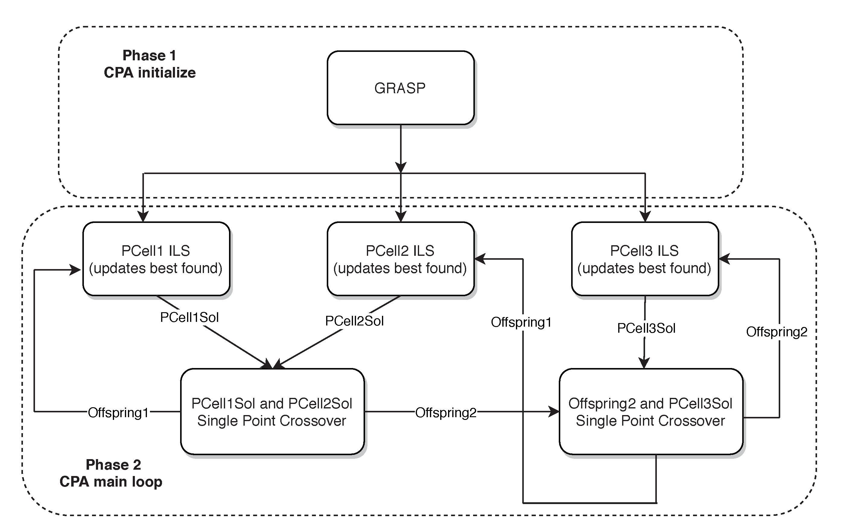
In a similar manner as in EFT-ILS, our proposed algorithm GRASP-CPA consists of two phases (see Figure 2). First, a GRASP explores feasible tasks’ orders for the next phase of the algorithm. In the second phase, the algorithm uses the best order $o_{best}$ and solution $s_{best}$ found by GRASP, in a homogeneous Cellular Processing Algorithm (CPA). The algorithm is composed by three ILS Processing Cells (PCells), the PCells have two functions that are independent from their ILS procedure. The first is to update the global best solution $s_{best}$ if the PCell finds a better solution. The second is to update their current solutions through the communication processes. The communication is performed using the well-known single point-crossover from Genetic Algorithms (GAs), where two solutions from different PCells split and combine their information [12,34]. This phase continues until a fixed number of iterations or CPU seconds is reached.

Algorithm 7 describes our GRASP-CPA proposal, where the $GRASPConstruction$ produces feasible orderings $o^{\prime }$ that are evaluated using $EFT$ to produce the solution $s^{\prime }$ (see lines 5 and 6). Here, we can see that the algorithm uses a $GRASPConstruction$ that receives an $\alpha$ value that can be either 0.9 or 1 with the same probability. This $\alpha$ value is used to restrict the candidate list (see lines 9 and 10 from Algorithm 3). GRASP algorithms usually use $\alpha$ values between 0.1 and 0.3. However, preliminary experimentation proved that the our proposed $\alpha$ values where the ones with the best performance for the instances used. Finally, line 12 executes the cellular processing section of the algorithm.

Algorithm 7 GRASP-CPA
Input:  $G=(T,C)$, computational costs $P_{i,j}$.
Output:  $s_{best}$, $o_{best}$
1: $s^{\prime }\leftarrow$ Random initial solution
2: $s_{best}\leftarrow s^{\prime }$
3: for $i=1$ to $MaxIterations$ do
4:     $\alpha \leftarrow randomFrom(0.9,1.0)$
5:     $o^{\prime }\leftarrow GRASPConstruction\left(\alpha \right)$
6:     $s^{\prime }\leftarrow EFT\left(o^{\prime }\right)$.
7:     if $f\left(s^{\prime }\right)<f\left(s_{best}\right)$ then
8:         $s_{best}\leftarrow s^{\prime }$
9:         $o_{best}\leftarrow o^{\prime }$
10:     end if
11: end for	▹ If the external stopping criterion is reach stop the for loop
12: $CPA(s_{best},o_{best})$.

Algorithm 8 Cellular Processing Algorithm section of the algorithm (GRASP-CPA)

Input:  $s_{best}$, $o_{best}$

Output:   $s_{best}$

1:  $PCell{1}_{s_{current}}\leftarrow s_{best}$

2:  $PCell{2}_{s_{current}}\leftarrow s_{best}$

3:  $PCell{3}_{s_{current}}\leftarrow s_{best}$

4: while stopping criterion not reached do

5:     $PCell1ILS\left(PCell{1}_{s_{current}}\right)$

6:     $PCell2ILS\left(PCell{2}_{s_{current}}\right)$

7:     $PCell3ILS\left(PCell{3}_{s_{current}}\right)$

8:     $Communication(PCell{1}_{s_{current}},PCell{2}_{s_{current}},PCell{3}_{s_{current}})$

9:  end while

Algorithm 8 shows the general idea of the $CPA(s_{best},o_{best})$ function. Here, the execution of the ILS Processing Cells (see lines 5 and 7) iterate five times each one, which limits the inner computational effort of the Processing Cells. After the Processing Cells’ execution, the $Communication$ processes the current solutions, recombining the $s_{best}$ of PCell1 with the $s_{best}$ of PCell2, the first offspring becomes the new current solution in PCell1. At the same time, the second offspring is used for a second recombination with the $s_{best}$ of PCell3. The resulting offsprings from the second recombination become the new current solution of PCell2 and PCell3. This process continues until the stopping criterion is reached (see line 4).

4. Experimental Setup

This section describes the experimental set of instances, the experimental configuration, and the statistical indicators of confidence in the results.

4.1. Parallel Application Instances

The applications used in the experimentation are:

• Double precision floating point FORTRAN benchmark (Fpppp) [35].
• The Laser Interferometer Gravitational-Wave Observatory (LIGO) application [36].
• Robot control application (Robot)
• Sparse matrix solver (Sparse).
• A benchmark of fourteen small synthetic instances from [11].

The applications Fpppp, Robot, and Sparse are included in the Standard Task Graph Set (STG) in [37]. We performed the same treatment to the original applications instances as in [8], considering different (Communication to Computation Ratios, CCRs) CCRs $=\{0.1,0.5,1,5,10\}$, (Heterogeneity Factors) HFs $=\{0.1,0.25,0.5,0.75,1\}$, and number of machines $\left|M\right|=\{8,16,32,64\}$. The combination of the mentioned configurations for the four parallel applications gives a total of $4·5·5·4=400$ instances. The nomenclature for the large instance set of Fpppp, Robot, and Sparse instances used in this work is Application-Machines-Tasks-HF-CCR. For the small benchmark in [11], the nomenclature is Name-Machines-Tasks. We made available the complete instance set in [38].

4.2. Experimental Settings

In the case of EFT-ILS, we use the best configuration in [11] (see

Table 3. Parameter settings for EFT-ILS and GRASP-CPA.

	EFT-ILS	GRASP-CPA
Phase 1 stopping criterion:	50 iterations/5 min	50 iterations/5 min
Phase 2 stopping criterion:	100,000 MaxEvaluations	100,000 MaxEvaluations
α:	-	$1.0$ and $0.9$
Communication:	-	single-point cx, $p_r=1.0$
ILS max iterations:	unlimited/MaxEvaluations	5/MaxEvaluations
Perturbation:	Section 3.3.2, $P_m=0.05$	Section 3.3.2, $P_m=0.05$
Local Search	Algorithm 6	Algorithm 6

). The GRASP-CPA uses a few extra parameters. One of them is the $\alpha$ value of the GRASP algorithm, for which we carried out extensive experimentation with $\alpha =\{0.1,0.2,0.3,0.4,0.5,0.6,0.7,0.8,0.9,1.0\}$, finding that the best values for these instances were 1.0 and 0.9 without a clear dominance. Thus, we decide to use 1.0 and 0.9 as $\alpha$ values randomly with an equal probability before the $GRASPConstruction$ (see line 5 of Algorithm 5). We use the same Local Search, perturbation process, and perturbation probability $p_m$ in both algorithms for a fair comparison. Finally, to ensure the CPA communication process, we set the probability of recombination $p_r$ as 100%. In both algorithms, the first phase has two stopping criteria, 50 iterations or a maximum of 5 min, while the second phase uses a stopping criterion of 100,000 objective function evaluations. Every instance from Section 4.1 is run 100 independent times. The complete experimental parameter settings are shown in Table 3. We made available the algorithm implementations at [39,40].

4.3. Statistical Indicators

To assess statistical confidence in our experimentation, we compute the median value from the independent runs as well as the interquartile range (IQR). The tables presenting our results follow the format $MEDIA{N}_{IQR}$. The tables also emphasize the best and second-best reported values for every problem with a gray and light background, respectively. For the sake of completeness, we apply the non-parametric Wilcoxon signed ranks test on the results to assess statistical differences in a pairwise comparison for every problem, at 95% confidence level [41]. A symbol ▲ indicates that EFT-ILS was statistically worse than GRASP-CPA according to the Wilcoxon signed ranks test; we use ▽ otherwise. Finally, we marked as ‘–’ the cases where there were no statistical differences.

5. Results

First, we start analyzing the results of the large benchmark set of 400 scheduling problems. Focusing on the Fpppp instance set (see

Table 4. Fpppp instances median and IQR of EFT-ILS and GRASP-CPA over 100 independent runs. Light gray emphasizes the best results.

Problem	EFT-ILS	GRASP-CPA	Problem	EFT-ILS	GRASP-CPA
Fpppp-8-334-0.1-0.1	$9.40E{1}_{1.1E0}-$	$9.39E{1}_{1.2E0}$	Fpppp-32-334-0.1-0.1	$2.28E{2}_{8.4E0}-$	$2.28E{2}_{6.8E0}$
Fpppp-8-334-0.1-0.5	$6.05E{2}_{9.8E0}▲$	$6.00E{2}_{8.7E0}$	Fpppp-32-334-0.1-0.5	$8.88E{2}_{2.1E1}▿$	$8.93E{2}_{3.2E1}$
Fpppp-8-334-0.1-1	$1.49E{3}_{2.5E1}▲$	$1.48E{3}_{2.7E1}$	Fpppp-32-334-0.1-1	$1.12E{3}_{3.0E1}▲$	$1.12E{3}_{2.5E1}$
Fpppp-8-334-0.1-5	$2.65E{3}_{9.2E1}▲$	$2.60E{3}_{8.8E1}$	Fpppp-32-334-0.1-5	$1.55E{3}_{7.0E1}▲$	$1.52E{3}_{7.6E1}$
Fpppp-8-334-0.1-10	$2.12E{3}_{7.7E1}▲$	$2.05E{3}_{9.7E1}$	Fpppp-32-334-0.1-10	$5.66E{3}_{2.7E2}▲$	$5.51E{3}_{3.2E2}$
Fpppp-8-334-0.25-0.1	$8.67E{2}_{1.1E1}▲$	$8.61E{2}_{1.1E1}$	Fpppp-32-334-0.25-0.1	$8.44E{2}_{2.8E1}-$	$8.40E{2}_{3.3E1}$
Fpppp-8-334-0.25-0.5	$2.65E{3}_{3.7E1}▲$	$2.64E{3}_{3.7E1}$	Fpppp-32-334-0.25-0.5	$5.71E{2}_{1.4E1}▿$	$5.75E{2}_{1.6E1}$
Fpppp-8-334-0.25-1	$1.94E{3}_{3.0E1}▲$	$1.93E{3}_{3.3E1}$	Fpppp-32-334-0.25-1	$2.66E{2}_{8.5E0}-$	$2.67E{2}_{6.8E0}$
Fpppp-8-334-0.25-5	$5.86E{2}_{2.1E1}▲$	$5.73E{2}_{2.4E1}$	Fpppp-32-334-0.25-5	$2.76E{3}_{1.5E2}▲$	$2.70E{3}_{1.3E2}$
Fpppp-8-334-0.25-10	$2.82E{3}_{1.2E2}▲$	$2.70E{3}_{1.3E2}$	Fpppp-32-334-0.25-10	$4.42E{3}_{1.6E2}-$	$4.41E{3}_{1.7E2}$
Fpppp-8-334-0.5-0.1	$3.87E{2}_{4.7E0}▲$	$3.83E{2}_{5.6E0}$	Fpppp-32-334-0.5-0.1	$1.04E{3}_{3.6E1}-$	$1.03E{3}_{3.4E1}$
Fpppp-8-334-0.5-0.5	$2.25E{3}_{3.9E1}▲$	$2.23E{3}_{3.8E1}$	Fpppp-32-334-0.5-0.5	$1.23E{3}_{4.1E1}▿$	$1.24E{3}_{4.2E1}$
Fpppp-8-334-0.5-1	$2.07E{3}_{4.4E1}▲$	$2.06E{3}_{4.2E1}$	Fpppp-32-334-0.5-1	$6.64E{2}_{1.8E1}-$	$6.66E{2}_{1.6E1}$
Fpppp-8-334-0.5-5	$4.23E{3}_{1.4E2}▲$	$4.08E{3}_{1.3E2}$	Fpppp-32-334-0.5-5	$2.41E{3}_{1.5E2}-$	$2.41E{3}_{1.4E2}$
Fpppp-8-334-0.5-10	$2.73E{3}_{1.3E2}▲$	$2.60E{3}_{1.5E2}$	Fpppp-32-334-0.5-10	$3.08E{3}_{1.2E2}▲$	$3.03E{3}_{1.1E2}$
Fpppp-8-334-0.75-0.1	$3.00E{2}_{5.8E0}▲$	$2.96E{2}_{4.8E0}$	Fpppp-32-334-0.75-0.1	$8.78E{2}_{3.1E1}▲$	$8.71E{2}_{3.1E1}$
Fpppp-8-334-0.75-0.5	$3.93E{2}_{8.4E0}▲$	$3.89E{2}_{6.0E0}$	Fpppp-32-334-0.75-0.5	$1.28E{3}_{2.7E1}-$	$1.28E{3}_{2.8E1}$
Fpppp-8-334-0.75-1	$7.64E{2}_{1.7E1}▲$	$7.53E{2}_{1.4E1}$	Fpppp-32-334-0.75-1	$7.89E{2}_{2.3E1}-$	$7.97E{2}_{1.9E1}$
Fpppp-8-334-0.75-5	$2.87E{3}_{1.3E2}▲$	$2.77E{3}_{1.4E2}$	Fpppp-32-334-0.75-5	$8.48E{2}_{3.1E1}▲$	$8.38E{2}_{2.4E1}$
Fpppp-8-334-0.75-10	$4.92E{3}_{1.9E2}▲$	$4.74E{3}_{2.4E2}$	Fpppp-32-334-0.75-10	$2.54E{3}_{7.0E1}▲$	$2.51E{3}_{7.3E1}$
Fpppp-8-334-1-0.1	$7.97E{2}_{1.1E1}▲$	$7.86E{2}_{1.0E1}$	Fpppp-32-334-1-0.1	$6.90E{2}_{2.2E1}-$	$6.90E{2}_{2.4E1}$
Fpppp-8-334-1-0.5	$1.31E{3}_{3.3E1}▲$	$1.30E{3}_{2.3E1}$	Fpppp-32-334-1-0.5	$6.28E{2}_{2.3E1}-$	$6.29E{2}_{1.8E1}$
Fpppp-8-334-1-1	$3.21E{2}_{7.3E0}▲$	$3.16E{2}_{8.4E0}$	Fpppp-32-334-1-1	$6.81E{1}_{1.7E0}-$	$6.82E{1}_{1.8E0}$
Fpppp-8-334-1-5	$4.63E{3}_{2.0E2}▲$	$4.53E{3}_{2.2E2}$	Fpppp-32-334-1-5	$2.13E{3}_{1.1E2}-$	$2.13E{3}_{8.0E1}$
Fpppp-8-334-1-10	$3.35E{3}_{1.4E2}▲$	$3.21E{3}_{1.0E2}$	Fpppp-32-334-1-10	$4.46E{3}_{2.5E2}▲$	$4.34E{3}_{1.9E2}$
Fpppp-16-334-0.1-0.1	$3.70E{2}_{7.7E0}-$	$3.72E{2}_{9.6E0}$	Fpppp-64-334-0.1-0.1	$2.60E{2}_{1.7E0}▲$	$2.60E{2}_{1.4E0}$
Fpppp-16-334-0.1-0.5	$1.93E{3}_{6.5E1}-$	$1.92E{3}_{7.8E1}$	Fpppp-64-334-0.1-0.5	$5.54E{1}_{8.4E-1}▿$	$5.58E{1}_{7.8E-1}$
Fpppp-16-334-0.1-1	$8.72E{2}_{2.7E1}▲$	$8.66E{2}_{3.4E1}$	Fpppp-64-334-0.1-1	$7.31E{2}_{1.1E1}▿$	$7.36E{2}_{1.0E1}$
Fpppp-16-334-0.1-5	$3.26E{3}_{1.2E2}-$	$3.25E{3}_{1.2E2}$	Fpppp-64-334-0.1-5	$2.00E{3}_{1.0E2}▿$	$2.03E{3}_{9.2E1}$
Fpppp-16-334-0.1-10	$5.57E{3}_{2.4E2}▲$	$5.37E{3}_{3.0E2}$	Fpppp-64-334-0.1-10	$2.26E{3}_{1.1E2}▿$	$2.28E{3}_{1.3E2}$
Fpppp-16-334-0.25-0.1	$1.80E{3}_{4.2E1}▲$	$1.78E{3}_{4.5E1}$	Fpppp-64-334-0.25-0.1	$8.93E{2}_{5.2E0}▿$	$8.97E{2}_{6.1E0}$
Fpppp-16-334-0.25-0.5	$1.78E{3}_{5.7E1}-$	$1.78E{3}_{6.0E1}$	Fpppp-64-334-0.25-0.5	$1.33E{3}_{1.4E1}▿$	$1.34E{3}_{1.6E1}$
Fpppp-16-334-0.25-1	$5.15E{2}_{2.5E1}-$	$5.12E{2}_{1.6E1}$	Fpppp-64-334-0.25-1	$9.48E{2}_{2.0E1}-$	$9.52E{2}_{2.6E1}$
Fpppp-16-334-0.25-5	$1.87E{3}_{7.0E1}▲$	$1.85E{3}_{7.9E1}$	Fpppp-64-334-0.25-5	$2.06E{3}_{9.9E1}-$	$2.06E{3}_{9.6E1}$
Fpppp-16-334-0.25-10	$8.07E{2}_{3.3E1}▲$	$7.79E{2}_{3.1E1}$	Fpppp-64-334-0.25-10	$1.74E{3}_{7.6E1}-$	$1.75E{3}_{8.1E1}$
Fpppp-16-334-0.5-0.1	$1.46E{3}_{3.0E1}▲$	$1.44E{3}_{2.6E1}$	Fpppp-64-334-0.5-0.1	$2.04E{2}_{3.3E-1}▲$	$2.04E{2}_{1.5E0}$
Fpppp-16-334-0.5-0.5	$1.35E{3}_{3.6E1}-$	$1.35E{3}_{4.0E1}$	Fpppp-64-334-0.5-0.5	$1.13E{3}_{1.1E1}▲$	$1.13E{3}_{1.2E1}$
Fpppp-16-334-0.5-1	$3.80E{2}_{1.4E1}▲$	$3.74E{2}_{1.1E1}$	Fpppp-64-334-0.5-1	$5.96E{2}_{1.1E1}▲$	$6.01E{2}_{7.4E0}$
Fpppp-16-334-0.5-5	$2.82E{3}_{1.7E2}-$	$2.85E{3}_{1.3E2}$	Fpppp-64-334-0.5-5	$1.23E{3}_{6.1E1}▲$	$1.26E{3}_{6.0E1}$
Fpppp-16-334-0.5-10	$9.22E{2}_{2.9E1}▲$	$8.94E{2}_{3.4E1}$	Fpppp-64-334-0.5-10	$1.61E{3}_{6.8E1}-$	$1.62E{3}_{5.4E1}$
Fpppp-16-334-0.75-0.1	$3.27E{2}_{7.2E0}▲$	$3.24E{2}_{9.2E0}$	Fpppp-64-334-0.75-0.1	$1.18E{2}_{8.0E-2}▲$	$1.18E{2}_{6.7E-1}$
Fpppp-16-334-0.75-0.5	$5.87E{2}_{2.2E1}-$	$5.85E{2}_{1.7E1}$	Fpppp-64-334-0.75-0.5	$4.72E{2}_{9.2E0}▿$	$4.76E{2}_{1.1E1}$
Fpppp-16-334-0.75-1	$6.12E{2}_{2.2E1}-$	$6.12E{2}_{2.0E1}$	Fpppp-64-334-0.75-1	$4.98E{2}_{1.2E1}-$	$5.00E{2}_{1.1E1}$
Fpppp-16-334-0.75-5	$3.73E{3}_{2.6E2}▲$	$3.68E{3}_{1.9E2}$	Fpppp-64-334-0.75-5	$8.96E{2}_{4.9E1}-$	$9.06E{2}_{5.3E1}$
Fpppp-16-334-0.75-10	$1.99E{3}_{1.0E2}▲$	$1.92E{3}_{8.2E1}$	Fpppp-64-334-0.75-10	$3.44E{3}_{1.4E2}-$	$3.46E{3}_{1.4E2}$
Fpppp-16-334-1-0.1	$7.48E{2}_{1.8E1}▲$	$7.40E{2}_{1.7E1}$	Fpppp-64-334-1-0.1	$8.22E{1}_{5.2E-1}▿$	$8.26E{1}_{6.8E-1}$
Fpppp-16-334-1-0.5	$9.56E{2}_{2.7E1}-$	$9.47E{2}_{2.8E1}$	Fpppp-64-334-1-0.5	$3.55E{2}_{3.8E0}▿$	$3.56E{2}_{2.5E0}$
Fpppp-16-334-1-1	$4.58E{2}_{1.3E1}▲$	$4.54E{2}_{1.5E1}$	Fpppp-64-334-1-1	$1.28E{3}_{1.2E1}▿$	$1.29E{3}_{1.4E1}$
Fpppp-16-334-1-5	$1.45E{3}_{6.4E1}-$	$1.44E{3}_{6.8E1}$	Fpppp-64-334-1-5	$8.50E{2}_{5.1E1}-$	$8.58E{2}_{5.8E1}$
Fpppp-16-334-1-10	$9.84E{2}_{3.5E1}▲$	$9.54E{2}_{4.2E1}$	Fpppp-64-334-1-10	$4.34E{3}_{1.6E2}▿$	$4.39E{3}_{1.8E2}$

▲ GRASP-CPA outperforms EFT-ILS with statistical difference, otherwise ▽, − no statistical difference.

), GRASP-CPA outperformed with statistical significance EFT-ILS in 53 instances, not statistically outperforming in any instance with 8 and 16 machines. However, for the instances with 32 and 64 machines, EFT-ILS outperformed GRASP-CPA in 3 and 11 instances, respectively.

Regarding the LIGO benchmark results from

Table 5. LIGO instances median and IQR of EFT-ILS and GRASP-CPA over 100 independent runs. Light gray emphasizes the best results.

Problem	EFT-ILS	GRASP-CPA	Problem	EFT-ILS	GRASP-CPA
LIGO-8-76-0.1-0.1	$6.10E{2}_{1.9E1}▲$	$6.08E{2}_{1.4E1}$	LIGO-32-76-0.1-0.1	$5.40E{2}_{1.4E0}▿$	$5.41E{2}_{1.3E0}$
LIGO-8-76-0.1-0.5	$9.24E{2}_{1.8E1}-$	$9.20E{2}_{2.0E1}$	LIGO-32-76-0.1-0.5	$6.00E{2}_{1.2E1}▿$	$6.02E{2}_{1.3E1}$
LIGO-8-76-0.1-1	$1.04E{3}_{2.5E1}▲$	$1.03E{3}_{3.8E1}$	LIGO-32-76-0.1-1	$3.03E{1}_{8.5E-1}-$	$3.03E{1}_{8.3E-1}$
LIGO-8-76-0.1-5	$1.36E{3}_{5.2E1}▲$	$1.30E{3}_{7.1E1}$	LIGO-32-76-0.1-5	$1.30E{3}_{6.3E1}▲$	$1.26E{3}_{8.7E1}$
LIGO-8-76-0.1-10	$1.48E{3}_{7.5E1}▲$	$1.46E{3}_{1.1E2}$	LIGO-32-76-0.1-10	$2.01E{3}_{1.2E2}▲$	$1.96E{3}_{1.1E2}$
LIGO-8-76-0.25-0.1	$4.91E{2}_{1.4E1}▲$	$4.82E{2}_{1.1E1}$	LIGO-32-76-0.25-0.1	$1.03E{2}_{8.1E-1}-$	$1.03E{2}_{7.2E-1}$
LIGO-8-76-0.25-0.5	$7.54E{2}_{2.4E1}▲$	$7.49E{2}_{1.8E1}$	LIGO-32-76-0.25-0.5	$8.64E{1}_{1.5E0}▲$	$8.59E{1}_{2.4E0}$
LIGO-8-76-0.25-1	$4.76E{2}_{1.7E1}▲$	$4.70E{2}_{1.2E1}$	LIGO-32-76-0.25-1	$8.43E{2}_{2.2E1}-$	$8.42E{2}_{2.7E1}$
LIGO-8-76-0.25-5	$2.15E{2}_{8.1E0}▲$	$2.11E{2}_{9.3E0}$	LIGO-32-76-0.25-5	$5.86E{2}_{2.0E1}-$	$5.82E{2}_{2.3E1}$
LIGO-8-76-0.25-10	$1.74E{3}_{1.2E2}▲$	$1.71E{3}_{8.4E1}$	LIGO-32-76-0.25-10	$8.25E{2}_{5.9E1}▲$	$8.06E{2}_{6.4E1}$
LIGO-8-76-0.5-0.1	$4.30E{2}_{1.1E1}▲$	$4.24E{2}_{1.1E1}$	LIGO-32-76-0.5-0.1	$6.76E{2}_{0.0E0}-$	$6.76E{2}_{0.0E0}$
LIGO-8-76-0.5-0.5	$8.17E{2}_{2.4E1}▲$	$8.05E{2}_{2.6E1}$	LIGO-32-76-0.5-0.5	$3.72E{2}_{8.4E0}▿$	$3.77E{2}_{1.0E1}$
LIGO-8-76-0.5-1	$8.06E{2}_{2.6E1}▿$	$8.15E{2}_{3.0E1}$	LIGO-32-76-0.5-1	$4.22E{2}_{1.3E1}-$	$4.22E{2}_{1.3E1}$
LIGO-8-76-0.5-5	$1.77E{3}_{1.1E2}-$	$1.76E{3}_{8.6E1}$	LIGO-32-76-0.5-5	$6.40E{2}_{3.2E1}▲$	$6.33E{2}_{3.3E1}$
LIGO-8-76-0.5-10	$3.41E{2}_{2.6E1}▿$	$3.46E{2}_{2.3E1}$	LIGO-32-76-0.5-10	$1.70E{3}_{1.0E2}▲$	$1.63E{3}_{6.1E1}$
LIGO-8-76-0.75-0.1	$1.75E{2}_{3.7E0}▲$	$1.71E{2}_{4.5E0}$	LIGO-32-76-0.75-0.1	$5.70E{2}_{0.0E0}-$	$5.70E{2}_{0.0E0}$
LIGO-8-76-0.75-0.5	$5.19E{2}_{1.6E1}▲$	$5.09E{2}_{1.4E1}$	LIGO-32-76-0.75-0.5	$3.19E{2}_{1.4E0}-$	$3.19E{2}_{1.2E0}$
LIGO-8-76-0.75-1	$7.62E{2}_{2.6E1}▲$	$7.52E{2}_{2.0E1}$	LIGO-32-76-0.75-1	$6.60E{1}_{1.5E0}▿$	$6.61E{1}_{1.0E0}$
LIGO-8-76-0.75-5	$4.78E{2}_{2.6E1}▲$	$4.71E{2}_{2.5E1}$	LIGO-32-76-0.75-5	$1.42E{3}_{5.5E1}▲$	$1.39E{3}_{9.4E1}$
LIGO-8-76-0.75-10	$9.21E{2}_{4.2E1}▲$	$8.73E{2}_{6.3E1}$	LIGO-32-76-0.75-10	$1.46E{3}_{7.0E1}▲$	$1.44E{3}_{8.4E1}$
LIGO-8-76-1-0.1	$1.41E{2}_{3.8E0}▲$	$1.36E{2}_{3.0E0}$	LIGO-32-76-1-0.1	$4.23E{2}_{0.0E0}-$	$4.23E{2}_{0.0E0}$
LIGO-8-76-1-0.5	$4.13E{2}_{1.3E1}-$	$4.16E{2}_{1.1E1}$	LIGO-32-76-1-0.5	$1.09E{2}_{2.9E0}▿$	$1.10E{2}_{2.3E0}$
LIGO-8-76-1-1	$8.08E{2}_{2.0E1}-$	$8.09E{2}_{1.7E1}$	LIGO-32-76-1-1	$1.59E{2}_{3.5E0}-$	$1.59E{2}_{4.5E0}$
LIGO-8-76-1-5	$4.22E{2}_{2.3E1}▲$	$4.11E{2}_{2.1E1}$	LIGO-32-76-1-5	$5.48E{2}_{4.0E1}▲$	$5.33E{2}_{3.2E1}$
LIGO-8-76-1-10	$2.75E{2}_{1.5E1}▲$	$2.68E{2}_{1.2E1}$	LIGO-32-76-1-10	$2.25E{3}_{2.6E2}▲$	$2.14E{3}_{1.2E2}$
LIGO-16-76-0.1-0.1	$5.52E{1}_{5.0E-1}▿$	$5.54E{1}_{9.8E-1}$	LIGO-64-76-0.1-0.1	$6.02E{2}_{4.5E-1}▲$	$6.02E{2}_{1.1E0}$
LIGO-16-76-0.1-0.5	$5.87E{2}_{7.0E0}▿$	$5.89E{2}_{6.8E0}$	LIGO-64-76-0.1-0.5	$4.22E{2}_{1.5E1}-$	$4.17E{2}_{1.4E1}$
LIGO-16-76-0.1-1	$7.78E{2}_{3.6E1}▿$	$7.85E{2}_{3.3E1}$	LIGO-64-76-0.1-1	$1.72E{2}_{3.7E0}▿$	$1.73E{2}_{3.8E0}$
LIGO-16-76-0.1-5	$1.28E{3}_{8.7E1}-$	$1.28E{3}_{8.7E1}$	LIGO-64-76-0.1-5	$1.10E{3}_{3.9E1}-$	$1.11E{3}_{4.9E1}$
LIGO-16-76-0.1-10	$2.23E{3}_{1.5E2}-$	$2.23E{3}_{1.7E2}$	LIGO-64-76-0.1-10	$1.32E{3}_{7.7E1}▲$	$1.27E{3}_{6.8E1}$
LIGO-16-76-0.25-0.1	$2.94E{2}_{0.0E0}▲$	$2.94E{2}_{4.5E-1}$	LIGO-64-76-0.25-0.1	$5.92E{1}_{6.8E-1}▿$	$5.93E{1}_{8.5E-1}$
LIGO-16-76-0.25-0.5	$2.98E{2}_{1.1E0}▲$	$2.97E{2}_{1.9E0}$	LIGO-64-76-0.25-0.5	$1.69E{2}_{1.9E0}-$	$1.69E{2}_{2.4E0}$
LIGO-16-76-0.25-1	$1.01E{2}_{1.5E0}-$	$1.02E{2}_{1.7E0}$	LIGO-64-76-0.25-1	$4.27E{2}_{1.7E1}▿$	$4.30E{2}_{1.2E1}$
LIGO-16-76-0.25-5	$1.02E{3}_{5.2E1}-$	$1.03E{3}_{4.5E1}$	LIGO-64-76-0.25-5	$1.68E{3}_{7.5E1}-$	$1.69E{3}_{8.0E1}$
LIGO-16-76-0.25-10	$5.77E{2}_{3.7E1}▲$	$5.57E{2}_{2.1E1}$	LIGO-64-76-0.25-10	$1.81E{3}_{9.3E1}▲$	$1.78E{3}_{8.9E1}$
LIGO-16-76-0.5-0.1	$1.35E{2}_{1.8E-1}-$	$1.35E{2}_{2.4E-1}$	LIGO-64-76-0.5-0.1	$6.26E{2}_{0.0E0}-$	$6.26E{2}_{0.0E0}$
LIGO-16-76-0.5-0.5	$3.62E{2}_{8.8E0}-$	$3.62E{2}_{7.4E0}$	LIGO-64-76-0.5-0.5	$6.21E{2}_{5.6E0}-$	$6.22E{2}_{2.7E0}$
LIGO-16-76-0.5-1	$9.26E{2}_{4.1E1}-$	$9.19E{2}_{3.4E1}$	LIGO-64-76-0.5-1	$3.26E{2}_{8.1E0}▲$	$3.22E{2}_{1.2E1}$
LIGO-16-76-0.5-5	$2.80E{2}_{9.2E0}-$	$2.81E{2}_{8.6E0}$	LIGO-64-76-0.5-5	$1.25E{3}_{7.8E1}-$	$1.27E{3}_{8.9E1}$
LIGO-16-76-0.5-10	$2.45E{2}_{1.7E1}-$	$2.42E{2}_{1.2E1}$	LIGO-64-76-0.5-10	$9.80E{2}_{5.5E1}▲$	$9.47E{2}_{5.3E1}$
LIGO-16-76-0.75-0.1	$4.93E{2}_{0.0E0}-$	$4.93E{2}_{0.0E0}$	LIGO-64-76-0.75-0.1	$2.72E{2}_{0.0E0}-$	$2.72E{2}_{0.0E0}$
LIGO-16-76-0.75-0.5	$1.65E{2}_{5.6E0}-$	$1.65E{2}_{4.2E0}$	LIGO-64-76-0.75-0.5	$2.79E{2}_{0.0E0}-$	$2.79E{2}_{0.0E0}$
LIGO-16-76-0.75-1	$3.78E{2}_{1.1E1}▲$	$3.76E{2}_{1.4E1}$	LIGO-64-76-0.75-1	$3.33E{2}_{1.4E1}▲$	$3.27E{2}_{9.3E0}$
LIGO-16-76-0.75-5	$1.09E{3}_{5.0E1}-$	$1.10E{3}_{6.0E1}$	LIGO-64-76-0.75-5	$8.42E{2}_{6.0E1}▲$	$8.17E{2}_{5.0E1}$
LIGO-16-76-0.75-10	$6.77E{2}_{4.5E1}-$	$6.74E{2}_{3.6E1}$	LIGO-64-76-0.75-10	$2.42E{3}_{1.2E2}▲$	$2.33E{3}_{9.7E1}$
LIGO-16-76-1-0.1	$1.11E{2}_{5.2E-1}▲$	$1.11E{2}_{1.3E0}$	LIGO-64-76-1-0.1	$3.01E{2}_{0.0E0}-$	$3.01E{2}_{0.0E0}$
LIGO-16-76-1-0.5	$1.34E{2}_{1.8E0}-$	$1.34E{2}_{1.7E0}$	LIGO-64-76-1-0.5	$2.55E{2}_{0.0E0}-$	$2.55E{2}_{0.0E0}$
LIGO-16-76-1-1	$2.85E{2}_{6.7E0}-$	$2.85E{2}_{4.7E0}$	LIGO-64-76-1-1	$1.63E{2}_{2.1E0}-$	$1.63E{2}_{2.1E0}$
LIGO-16-76-1-5	$1.39E{2}_{6.0E0}▲$	$1.38E{2}_{6.0E0}$	LIGO-64-76-1-5	$1.50E{3}_{8.2E1}-$	$1.51E{3}_{7.5E1}$
LIGO-16-76-1-10	$2.24E{2}_{2.4E1}▲$	$2.29E{2}_{2.3E1}$	LIGO-64-76-1-10	$1.20E{2}_{7.8E0}▲$	$1.18E{2}_{8.3E0}$

, GRASP-CPA outperformed EFT-ILS in 45 instances. EFT-ILS only outperformed GRASP-CPA in 13 instances, distributed as follows: two, three, five, and three for the instances with 8, 16, 32, and 64 machines, respectively.

For the Robot benchmark (see

Table 6. Robot instances median and IQR of EFT-ILS and GRASP-CPA over 100 independent runs. Light gray emphasizes the best results.

Problem	EFT-ILS	GRASP-CPA	Problem	EFT-ILS	GRASP-CPA
Robot-8-88-0.1-0.1	$1.89E{3}_{2.7E1}▲$	$1.88E{3}_{1.6E1}$	Robot-32-88-0.1-0.1	$1.07E{3}_{2.3E0}-$	$1.07E{3}_{2.3E0}$
Robot-8-88-0.1-0.5	$7.22E{1}_{1.3E0}-$	$7.20E{1}_{1.2E0}$	Robot-32-88-0.1-0.5	$1.07E{3}_{3.8E0}▲$	$1.06E{3}_{1.1E1}$
Robot-8-88-0.1-1	$2.02E{3}_{4.4E1}▲$	$1.98E{3}_{3.7E1}$	Robot-32-88-0.1-1	$1.32E{3}_{1.3E1}▿$	$1.33E{3}_{1.1E1}$
Robot-8-88-0.1-5	$3.03E{3}_{1.1E2}-$	$3.04E{3}_{1.0E2}$	Robot-32-88-0.1-5	$2.44E{3}_{9.8E1}▲$	$2.35E{3}_{1.0E2}$
Robot-8-88-0.1-10	$2.39E{3}_{1.0E2}▲$	$2.24E{3}_{9.0E1}$	Robot-32-88-0.1-10	$2.97E{2}_{1.1E1}▲$	$2.74E{2}_{1.1E1}$
Robot-8-88-0.25-0.1	$6.45E{2}_{1.1E1}▲$	$6.40E{2}_{9.3E0}$	Robot-32-88-0.25-0.1	$1.26E{3}_{3.0E0}-$	$1.26E{3}_{2.4E0}$
Robot-8-88-0.25-0.5	$6.52E{2}_{9.9E0}▲$	$6.50E{2}_{8.2E0}$	Robot-32-88-0.25-0.5	$8.73E{1}_{8.8E-1}▲$	$8.71E{1}_{8.9E-1}$
Robot-8-88-0.25-1	$4.71E{2}_{6.4E0}▿$	$4.73E{2}_{8.1E0}$	Robot-32-88-0.25-1	$1.91E{3}_{2.7E1}-$	$1.91E{3}_{2.6E1}$
Robot-8-88-0.25-5	$1.55E{3}_{4.5E1}-$	$1.56E{3}_{4.5E1}$	Robot-32-88-0.25-5	$3.05E{3}_{1.1E2}-$	$3.04E{3}_{8.9E1}$
Robot-8-88-0.25-10	$2.73E{3}_{9.6E1}▲$	$2.66E{3}_{8.2E1}$	Robot-32-88-0.25-10	$1.85E{3}_{8.2E1}▲$	$1.68E{3}_{7.6E1}$
Robot-8-88-0.5-0.1	$1.03E{3}_{1.6E1}▲$	$1.02E{3}_{1.3E1}$	Robot-32-88-0.5-0.1	$3.75E{2}_{2.7E0}▲$	$3.74E{2}_{7.7E-1}$
Robot-8-88-0.5-0.5	$7.93E{2}_{1.6E1}▲$	$7.85E{2}_{1.5E1}$	Robot-32-88-0.5-0.5	$3.23E{2}_{3.8E0}▲$	$3.21E{2}_{3.8E0}$
Robot-8-88-0.5-1	$7.45E{2}_{1.1E1}▲$	$7.41E{2}_{1.2E1}$	Robot-32-88-0.5-1	$8.58E{2}_{1.2E1}▿$	$8.65E{2}_{1.4E1}$
Robot-8-88-0.5-5	$1.35E{3}_{4.0E1}▲$	$1.34E{3}_{3.0E1}$	Robot-32-88-0.5-5	$7.28E{2}_{1.7E1}-$	$7.24E{2}_{1.8E1}$
Robot-8-88-0.5-10	$3.60E{2}_{1.8E1}▲$	$3.49E{2}_{1.4E1}$	Robot-32-88-0.5-10	$1.98E{3}_{7.2E1}-$	$1.99E{3}_{6.3E1}$
Robot-8-88-0.75-0.1	$5.64E{2}_{1.2E1}▲$	$5.60E{2}_{1.1E1}$	Robot-32-88-0.75-0.1	$9.42E{2}_{0.0E0}-$	$9.42E{2}_{1.5E0}$
Robot-8-88-0.75-0.5	$1.59E{3}_{2.1E1}▲$	$1.58E{3}_{1.7E1}$	Robot-32-88-0.75-0.5	$1.28E{3}_{1.5E1}-$	$1.28E{3}_{1.2E1}$
Robot-8-88-0.75-1	$1.40E{3}_{2.9E1}-$	$1.40E{3}_{2.2E1}$	Robot-32-88-0.75-1	$1.39E{3}_{1.3E1}-$	$1.39E{3}_{1.8E1}$
Robot-8-88-0.75-5	$2.52E{3}_{7.1E1}▲$	$2.41E{3}_{8.0E1}$	Robot-32-88-0.75-5	$1.50E{3}_{5.0E1}▿$	$1.51E{3}_{4.4E1}$
Robot-8-88-0.75-10	$1.09E{3}_{4.2E1}▲$	$1.04E{3}_{3.8E1}$	Robot-32-88-0.75-10	$4.75E{2}_{1.5E1}▲$	$4.56E{2}_{1.8E1}$
Robot-8-88-1-0.1	$3.04E{2}_{7.2E0}▲$	$2.96E{2}_{5.7E0}$	Robot-32-88-1-0.1	$1.02E{3}_{3.2E0}-$	$1.02E{3}_{3.2E0}$
Robot-8-88-1-0.5	$3.73E{2}_{9.3E0}▲$	$3.66E{2}_{8.0E0}$	Robot-32-88-1-0.5	$4.67E{2}_{0.0E0}-$	$4.67E{2}_{4.1E-1}$
Robot-8-88-1-1	$1.38E{3}_{4.0E1}▲$	$1.36E{3}_{4.3E1}$	Robot-32-88-1-1	$7.96E{2}_{2.3E1}▲$	$7.78E{2}_{3.2E1}$
Robot-8-88-1-5	$9.94E{2}_{2.8E1}-$	$9.95E{2}_{2.8E1}$	Robot-32-88-1-5	$1.16E{3}_{3.1E1}▲$	$1.14E{3}_{2.9E1}$
Robot-8-88-1-10	$2.01E{3}_{7.0E1}▲$	$1.93E{3}_{6.7E1}$	Robot-32-88-1-10	$1.39E{3}_{6.0E1}-$	$1.38E{3}_{4.5E1}$
Robot-16-88-0.1-0.1	$6.78E{2}_{3.5E0}-$	$6.78E{2}_{1.3E0}$	Robot-64-88-0.1-0.1	$2.13E{2}_{5.1E-1}-$	$2.13E{2}_{1.0E0}$
Robot-16-88-0.1-0.5	$1.91E{3}_{1.3E1}▿$	$1.92E{3}_{1.6E1}$	Robot-64-88-0.1-0.5	$8.75E{2}_{1.2E1}▿$	$8.78E{2}_{1.6E1}$
Robot-16-88-0.1-1	$1.15E{3}_{2.2E1}-$	$1.14E{3}_{2.4E1}$	Robot-64-88-0.1-1	$9.45E{2}_{1.2E1}-$	$9.46E{2}_{1.2E1}$
Robot-16-88-0.1-5	$5.16E{2}_{1.8E1}▿$	$5.19E{2}_{1.5E1}$	Robot-64-88-0.1-5	$2.55E{3}_{8.3E1}▲$	$2.50E{3}_{8.0E1}$
Robot-16-88-0.1-10	$2.53E{3}_{7.1E1}▲$	$2.46E{3}_{6.8E1}$	Robot-64-88-0.1-10	$3.27E{3}_{1.2E2}▲$	$3.17E{3}_{9.8E1}$
Robot-16-88-0.25-0.1	$6.00E{1}_{5.0E-1}▿$	$6.01E{1}_{5.3E-1}$	Robot-64-88-0.25-0.1	$1.35E{3}_{3.7E0}-$	$1.35E{3}_{5.4E-1}$
Robot-16-88-0.25-0.5	$3.67E{2}_{2.4E0}-$	$3.67E{2}_{2.1E0}$	Robot-64-88-0.25-0.5	$1.64E{3}_{1.7E1}-$	$1.64E{3}_{1.1E1}$
Robot-16-88-0.25-1	$5.48E{2}_{1.1E1}-$	$5.47E{2}_{8.2E0}$	Robot-64-88-0.25-1	$1.09E{3}_{1.0E1}-$	$1.09E{3}_{9.7E0}$
Robot-16-88-0.25-5	$3.78E{3}_{1.4E2}-$	$3.79E{3}_{1.2E2}$	Robot-64-88-0.25-5	$2.23E{3}_{7.3E1}-$	$2.22E{3}_{7.6E1}$
Robot-16-88-0.25-10	$3.53E{3}_{1.4E2}▲$	$3.46E{3}_{1.9E2}$	Robot-64-88-0.25-10	$1.72E{2}_{6.4E0}▲$	$1.69E{2}_{3.9E0}$
Robot-16-88-0.5-0.1	$9.34E{2}_{1.9E0}▿$	$9.35E{2}_{1.2E0}$	Robot-64-88-0.5-0.1	$3.57E{2}_{0.0E0}-$	$3.57E{2}_{0.0E0}$
Robot-16-88-0.5-0.5	$1.38E{3}_{2.0E1}-$	$1.37E{3}_{1.7E1}$	Robot-64-88-0.5-0.5	$1.10E{3}_{1.3E1}-$	$1.10E{3}_{1.3E1}$
Robot-16-88-0.5-1	$2.34E{2}_{2.8E0}▿$	$2.35E{2}_{2.7E0}$	Robot-64-88-0.5-1	$4.51E{2}_{4.0E0}▲$	$4.49E{2}_{5.6E0}$
Robot-16-88-0.5-5	$1.89E{3}_{7.5E1}-$	$1.89E{3}_{6.5E1}$	Robot-64-88-0.5-5	$1.79E{3}_{8.2E1}-$	$1.79E{3}_{7.7E1}$
Robot-16-88-0.5-10	$3.33E{3}_{1.1E2}▲$	$3.24E{3}_{1.1E2}$	Robot-64-88-0.5-10	$3.18E{3}_{1.1E2}▲$	$3.13E{3}_{9.4E1}$
Robot-16-88-0.75-0.1	$3.48E{2}_{3.6E-1}-$	$3.48E{2}_{7.4E-1}$	Robot-64-88-0.75-0.1	$8.15E{2}_{0.0E0}-$	$8.15E{2}_{0.0E0}$
Robot-16-88-0.75-0.5	$1.63E{2}_{1.6E0}▲$	$1.63E{2}_{1.6E0}$	Robot-64-88-0.75-0.5	$1.58E{3}_{1.3E1}▲$	$1.58E{3}_{5.7E0}$
Robot-16-88-0.75-1	$7.18E{2}_{2.0E1}▲$	$7.14E{2}_{1.9E1}$	Robot-64-88-0.75-1	$2.24E{2}_{5.0E0}▲$	$2.19E{2}_{5.5E0}$
Robot-16-88-0.75-5	$2.36E{2}_{7.6E0}▲$	$2.28E{2}_{6.9E0}$	Robot-64-88-0.75-5	$2.53E{3}_{9.0E1}▲$	$2.47E{3}_{6.5E1}$
Robot-16-88-0.75-10	$8.92E{2}_{4.6E1}-$	$8.98E{2}_{4.6E1}$	Robot-64-88-0.75-10	$4.92E{3}_{1.6E2}▲$	$4.86E{3}_{1.3E2}$
Robot-16-88-1-0.1	$2.81E{2}_{1.3E0}-$	$2.80E{2}_{1.0E0}$	Robot-64-88-1-0.1	$8.45E{2}_{0.0E0}-$	$8.45E{2}_{0.0E0}$
Robot-16-88-1-0.5	$5.14E{2}_{2.6E0}▿$	$5.15E{2}_{3.0E0}$	Robot-64-88-1-0.5	$9.58E{2}_{9.6E-1}▿$	$9.59E{2}_{3.1E0}$
Robot-16-88-1-1	$1.77E{3}_{3.6E1}-$	$1.77E{3}_{2.4E1}$	Robot-64-88-1-1	$2.47E{2}_{1.2E0}▲$	$2.45E{2}_{2.7E0}$
Robot-16-88-1-5	$1.15E{3}_{4.9E1}-$	$1.15E{3}_{4.5E1}$	Robot-64-88-1-5	$1.73E{3}_{4.1E1}▲$	$1.71E{3}_{5.6E1}$
Robot-16-88-1-10	$8.29E{2}_{2.9E1}▲$	$8.22E{2}_{2.9E1}$	Robot-64-88-1-10	$3.07E{3}_{1.3E2}▲$	$3.00E{3}_{1.1E2}$

), GRASP-CPA outperformed EFT-ILS with statistical significance in 48 cases, while EFT-ILS only outperformed GRASP-CPA in 12 instances, where most of them occurred for the instances with 16 machines.

The results for the Sparse benchmark from

Table 7. Sparse instances median and IQR of EFT-ILS and GRASP-CPA over 100 independent runs. Light gray emphasizes the best results.

Problem	EFT-ILS	GRASP-CPA	Problem	EFT-ILS	GRASP-CPA
Sparse-8-96-0.1-0.1	$2.63E{1}_{6.9E-1}-$	$2.63E{1}_{7.3E-1}$	Sparse-32-96-0.1-0.1	$3.70E{2}_{2.1E-1}-$	$3.70E{2}_{1.4E-1}$
Sparse-8-96-0.1-0.5	$2.68E{2}_{9.8E0}▲$	$2.72E{2}_{1.1E1}$	Sparse-32-96-0.1-0.5	$4.96E{2}_{1.5E1}-$	$4.94E{2}_{1.3E1}$
Sparse-8-96-0.1-1	$4.50E{2}_{2.0E1}-$	$4.56E{2}_{2.0E1}$	Sparse-32-96-0.1-1	$5.33E{2}_{2.2E1}▿$	$5.34E{2}_{1.2E1}$
Sparse-8-96-0.1-5	$7.65E{2}_{2.6E1}▲$	$7.56E{2}_{3.2E1}$	Sparse-32-96-0.1-5	$2.36E{2}_{3.4E0}-$	$2.36E{2}_{4.8E0}$
Sparse-8-96-0.1-10	$8.93E{2}_{4.0E1}-$	$8.89E{2}_{4.0E1}$	Sparse-32-96-0.1-10	$1.41E{3}_{5.8E0}▲$	$1.41E{3}_{7.8E0}$
Sparse-8-96-0.25-0.1	$5.10E{2}_{1.1E1}-$	$5.08E{2}_{1.3E1}$	Sparse-32-96-0.25-0.1	$1.95E{2}_{8.5E0}-$	$1.96E{2}_{7.6E0}$
Sparse-8-96-0.25-0.5	$2.20E{1}_{7.7E-1}-$	$2.21E{1}_{8.0E-1}$	Sparse-32-96-0.25-0.5	$1.41E{2}_{2.4E0}-$	$1.41E{2}_{4.2E0}$
Sparse-8-96-0.25-1	$3.28E{2}_{1.9E1}▿$	$3.30E{2}_{1.5E1}$	Sparse-32-96-0.25-1	$4.32E{2}_{1.2E1}-$	$4.33E{2}_{1.3E1}$
Sparse-8-96-0.25-5	$2.09E{2}_{9.2E0}▲$	$2.07E{2}_{9.8E0}$	Sparse-32-96-0.25-5	$6.10E{2}_{4.1E1}-$	$6.14E{2}_{4.6E1}$
Sparse-8-96-0.25-10	$1.46E{3}_{5.6E1}-$	$1.45E{3}_{4.6E1}$	Sparse-32-96-0.25-10	$7.48E{2}_{9.5E0}-$	$7.48E{2}_{7.2E0}$
Sparse-8-96-0.5-0.1	$8.45E{2}_{3.1E1}-$	$8.55E{2}_{3.5E1}$	Sparse-32-96-0.5-0.1	$3.68E{2}_{1.6E1}-$	$3.66E{2}_{1.3E1}$
Sparse-8-96-0.5-0.5	$8.47E{2}_{2.1E1}-$	$8.44E{2}_{3.0E1}$	Sparse-32-96-0.5-0.5	$3.47E{1}_{1.2E0}▲$	$3.42E{1}_{1.1E0}$
Sparse-8-96-0.5-1	$5.95E{2}_{2.0E1}-$	$5.98E{2}_{2.6E1}$	Sparse-32-96-0.5-1	$5.27E{2}_{1.7E1}-$	$5.23E{2}_{1.8E1}$
Sparse-8-96-0.5-5	$3.56E{1}_{1.6E0}▲$	$3.52E{1}_{1.2E0}$	Sparse-32-96-0.5-5	$3.54E{2}_{1.8E1}-$	$3.54E{2}_{1.2E1}$
Sparse-8-96-0.5-10	$5.73E{2}_{3.2E1}-$	$5.69E{2}_{2.4E1}$	Sparse-32-96-0.5-10	$4.28E{2}_{2.6E0}▲$	$4.27E{2}_{3.2E0}$
Sparse-8-96-0.75-0.1	$6.50E{2}_{1.3E1}▲$	$6.43E{2}_{1.7E1}$	Sparse-32-96-0.75-0.1	$1.20E{2}_{4.9E0}-$	$1.21E{2}_{4.9E0}$
Sparse-8-96-0.75-0.5	$2.67E{2}_{7.0E0}▲$	$2.64E{2}_{7.9E0}$	Sparse-32-96-0.75-0.5	$2.15E{2}_{5.0E0}-$	$2.15E{2}_{6.0E0}$
Sparse-8-96-0.75-1	$6.52E{2}_{2.3E1}▲$	$6.46E{2}_{2.1E1}$	Sparse-32-96-0.75-1	$2.25E{2}_{8.9E0}-$	$2.28E{2}_{6.6E0}$
Sparse-8-96-0.75-5	$9.51E{2}_{8.3E1}-$	$9.51E{2}_{8.1E1}$	Sparse-32-96-0.75-5	$3.59E{1}_{1.1E0}▲$	$3.58E{1}_{1.0E0}$
Sparse-8-96-0.75-10	$9.99E{2}_{7.1E1}▲$	$9.36E{2}_{6.0E1}$	Sparse-32-96-0.75-10	$6.68E{2}_{2.2E1}▲$	$6.61E{2}_{2.9E1}$
Sparse-8-96-1-0.1	$6.97E{2}_{1.6E1}▲$	$6.92E{2}_{1.5E1}$	Sparse-32-96-1-0.1	$2.98E{1}_{5.7E-1}-$	$2.99E{1}_{5.7E-1}$
Sparse-8-96-1-0.5	$6.47E{2}_{2.4E1}▲$	$6.30E{2}_{2.5E1}$	Sparse-32-96-1-0.5	$2.88E{2}_{7.3E0}-$	$2.88E{2}_{7.2E0}$
Sparse-8-96-1-1	$2.48E{2}_{1.1E1}-$	$2.47E{2}_{7.0E0}$	Sparse-32-96-1-1	$2.05E{2}_{7.2E0}▿$	$2.08E{2}_{6.4E0}$
Sparse-8-96-1-5	$5.41E{2}_{2.3E1}▲$	$5.34E{2}_{2.2E1}$	Sparse-32-96-1-5	$5.95E{2}_{3.2E1}▲$	$5.86E{2}_{1.9E1}$
Sparse-8-96-1-10	$1.96E{2}_{9.8E0}-$	$1.97E{2}_{1.3E1}$	Sparse-32-96-1-10	$1.01E{3}_{7.2E1}▲$	$9.81E{2}_{9.4E1}$
Sparse-16-96-0.1-0.1	$5.47E{2}_{1.5E1}-$	$5.46E{2}_{2.1E1}$	Sparse-64-96-0.1-0.1	$1.36E{2}_{4.2E-1}▿$	$1.37E{2}_{3.7E-2}$
Sparse-16-96-0.1-0.5	$3.55E{2}_{1.3E1}-$	$3.57E{2}_{1.3E1}$	Sparse-64-96-0.1-0.5	$4.74E{2}_{9.6E-1}▿$	$4.74E{2}_{2.7E0}$
Sparse-16-96-0.1-1	$4.59E{2}_{2.0E1}-$	$4.60E{2}_{1.3E1}$	Sparse-64-96-0.1-1	$3.12E{2}_{1.6E0}▿$	$3.15E{2}_{2.2E0}$
Sparse-16-96-0.1-5	$1.91E{2}_{5.7E0}▲$	$1.89E{2}_{5.8E0}$	Sparse-64-96-0.1-5	$3.30E{2}_{9.9E-1}▲$	$3.29E{2}_{1.2E0}$
Sparse-16-96-0.1-10	$5.54E{2}_{7.9E0}-$	$5.54E{2}_{8.4E0}$	Sparse-64-96-0.1-10	$1.39E{2}_{4.0E-1}▲$	$1.38E{2}_{2.2E-1}$
Sparse-16-96-0.25-0.1	$3.04E{2}_{1.1E1}-$	$3.05E{2}_{1.1E1}$	Sparse-64-96-0.25-0.1	$2.73E{2}_{2.2E-1}▲$	$2.73E{2}_{0.0E0}$
Sparse-16-96-0.25-0.5	$2.27E{2}_{9.6E0}-$	$2.28E{2}_{8.3E0}$	Sparse-64-96-0.25-0.5	$4.04E{2}_{4.6E0}▿$	$4.05E{2}_{1.1E0}$
Sparse-16-96-0.25-1	$2.75E{2}_{1.2E1}▿$	$2.78E{2}_{1.2E1}$	Sparse-64-96-0.25-1	$9.32E{1}_{2.5E-1}-$	$9.32E{1}_{9.5E-2}$
Sparse-16-96-0.25-5	$8.10E{2}_{3.4E1}-$	$8.07E{2}_{3.2E1}$	Sparse-64-96-0.25-5	$3.86E{2}_{3.0E1}▲$	$3.64E{2}_{1.9E1}$
Sparse-16-96-0.25-10	$1.09E{3}_{4.5E1}▲$	$1.06E{3}_{3.2E1}$	Sparse-64-96-0.25-10	$5.47E{2}_{4.6E-1}-$	$5.47E{2}_{4.6E-1}$
Sparse-16-96-0.5-0.1	$1.92E{2}_{8.4E0}-$	$1.94E{2}_{5.8E0}$	Sparse-64-96-0.5-0.1	$4.52E{2}_{2.0E0}-$	$4.52E{2}_{5.8E-1}$
Sparse-16-96-0.5-0.5	$2.80E{2}_{1.5E1}-$	$2.82E{2}_{8.6E0}$	Sparse-64-96-0.5-0.5	$1.26E{2}_{7.9E0}▲$	$1.21E{2}_{6.7E0}$
Sparse-16-96-0.5-1	$2.01E{2}_{9.3E0}-$	$2.04E{2}_{9.0E0}$	Sparse-64-96-0.5-1	$2.73E{2}_{3.4E0}▿$	$2.75E{2}_{2.5E0}$
Sparse-16-96-0.5-5	$7.70E{2}_{5.3E1}▲$	$7.59E{2}_{3.9E1}$	Sparse-64-96-0.5-5	$7.03E{2}_{1.0E1}-$	$7.00E{2}_{2.0E1}$
Sparse-16-96-0.5-10	$1.80E{3}_{2.3E1}-$	$1.80E{3}_{3.3E1}$	Sparse-64-96-0.5-10	$1.74E{3}_{0.0E0}▲$	$1.74E{3}_{0.0E0}$
Sparse-16-96-0.75-0.1	$3.53E{2}_{1.5E1}-$	$3.51E{2}_{1.5E1}$	Sparse-64-96-0.75-0.1	$2.89E{2}_{5.2E0}-$	$2.91E{2}_{5.2E0}$
Sparse-16-96-0.75-0.5	$2.93E{2}_{1.2E1}-$	$2.93E{2}_{9.4E0}$	Sparse-64-96-0.75-0.5	$3.57E{2}_{1.1E0}▲$	$3.57E{2}_{5.3E0}$
Sparse-16-96-0.75-1	$3.46E{2}_{1.5E1}▲$	$3.42E{2}_{1.4E1}$	Sparse-64-96-0.75-1	$3.68E{2}_{3.4E0}▿$	$3.72E{2}_{1.2E1}$
Sparse-16-96-0.75-5	$5.94E{2}_{1.7E1}-$	$5.95E{2}_{2.4E1}$	Sparse-64-96-0.75-5	$3.13E{2}_{2.2E0}-$	$3.13E{2}_{0.0E0}$
Sparse-16-96-0.75-10	$1.64E{3}_{3.8E1}-$	$1.63E{3}_{6.6E1}$	Sparse-64-96-0.75-10	$4.64E{2}_{3.3E0}-$	$4.64E{2}_{3.0E0}$
Sparse-16-96-1-0.1	$2.03E{2}_{7.2E0}-$	$2.01E{2}_{7.2E0}$	Sparse-64-96-1-0.1	$2.32E{2}_{0.0E0}-$	$2.32E{2}_{0.0E0}$
Sparse-16-96-1-0.5	$2.49E{2}_{1.2E1}-$	$2.50E{2}_{1.2E1}$	Sparse-64-96-1-0.5	$1.72E{2}_{4.4E0}-$	$1.72E{2}_{2.5E0}$
Sparse-16-96-1-1	$1.79E{2}_{8.0E0}-$	$1.78E{2}_{7.5E0}$	Sparse-64-96-1-1	$8.33E{1}_{0.0E0}▲$	$8.33E{1}_{0.0E0}$
Sparse-16-96-1-5	$3.73E{2}_{1.9E1}-$	$3.73E{2}_{2.0E1}$	Sparse-64-96-1-5	$4.10E{2}_{9.4E0}▲$	$4.07E{2}_{8.6E0}$
Sparse-16-96-1-10	$1.75E{3}_{5.2E1}▲$	$1.73E{3}_{4.9E1}$	Sparse-64-96-1-10	$1.65E{3}_{1.1E0}▲$	$1.65E{3}_{0.0E0}$

show that GRASP-CPA outperformed EFT-ILS with statistical significance in 33 instances, while EFT-ILS outperformed GRASP-CPA in 10 instances.

Finally, for these instances sets, GRASP-CPA achieved 265% more best median values found than EFT-ILS, with statistical significance. Therefore, we consider that GRASP-CPA is superior to EFT-ILS in a relevant proportion of the studied cases.

Furthermore, we analyze the results from the small benchmark of 14 synthetic instances in

Table 8. Small synthetic benchmark instances median and IQR of EFT-ILS and GRASP-CPA over 100 independent runs. Light gray emphasizes the best results.

Problem	EFT-ILS	GRASP-CPA	Optimum	Reference	Time${}_{\mathbf{Enum}}$	Time${}_{\mathbf{EFT-ILS}}$	Time${}_{\mathbf{GRASP-CPA}}$
Ahmad-3-9	${27}_{0.0}-$	${27}_{0.0}$	27	[42]	8s	0s	0s
Daoud-2-11	${60}_{1.5}▲$	$58.5_{4.0}$	56	[43]	46s	0s	0s
Eswari-2-11	${60}_{0.5}▲$	$58.5_{4.0}$	56	[44]	46s	0s	0s
Hamid-3-10	${100}_{0.0}-$	${100}_{0.0}$	100	[45]	71s	0s	0s
Heteropar-4-12	${136}_{0.0}▲$	${124}_{12}$	124	[46]	1677s	0s	0s
Hsu-3-10	${80}_{0.0}▲$	${80}_{0.0}$	80	[47]	64s	0s	0s
Ilavarasan-3-10	${73}_{3.0}▲$	${73}_{0.0}$	73	[48]	65s	0s	0s
Kang1-3-10	${76}_{0.0}▲$	${76}_{1.0}$	73	[49]	67s	0s	0s
Kang2-3-10	${83}_{0.0}▲$	${83}_{0.0}$	79	[50]	68s	0s	0s
Kuan-3-10	${27}_{0.0}▲$	${27}_{0.0}$	26	[51]	25s	0s	0s
Liang-3-10	${73}_{3.0}▲$	${73}_{3.0}$	73	[52]	67s	0s	0s
Sample-3-8	${84}_{2.0}▲$	${82}_{3.0}$	81	[11]	0s	0s	0s
SampleFig-3-8	${66}_{0.0}-$	${66}_{0.0}$	66	[11]	0s	0s	0s
YCLee-3-8	${66}_{0.0}-$	${66}_{0.0}$	66	[53]	0s	0s	0s

. For the 14 synthetic problems, GRASP-CPA achieves the best median value in all the cases, with statistical significance in ten cases. In addition, Table 8 shows the average computing time of the enumerative optimal algorithm (Time${}_{\mathrm{Enum}}$), EFT-ILS (Time${}_{\mathrm{EFT-ILS}}$), and GRASP-CPA (Time${}_{\mathrm{GRASP-CPA}}$) in CPU seconds on a Macbook pro 13-inch late 2011.

Table 9. Small synthetic benchmark instances best results found by EFT-ILS and GRASP-CPA over 100 independent runs. Light gray emphasizes the best results.

Problem	EFT-ILS	GRASP-CPA	Optimum	Reference
Ahmad-3-9	27	27	27	[42]
Daoud-2-11	56	56	56	[43]
Eswari-2-11	56	56	56	[44]
Hamid-3-10	100	100	100	[45]
Heteropar-4-12	136	124	124	[46]
Hsu-3-10	80	80	80	[47]
Ilavarasan-3-10	73	73	73	[48]
Kang1-3-10	73	73	73	[49]
Kang2-3-10	83	82	79	[50]
Kuan-3-10	26	26	26	[51]
Liang-3-10	73	73	73	[52]
Sample-3-8	81	81	81	[11]
SampleFig-3-8	66	66	66	[11]
YCLee-3-8	66	66	66	[53]

presents the best solution found by EFT-ILS and GRASP-CPA, where EFT-ILS computes twelve optimal values, while GRASP-CPA computes 13. Additionally, GRASP-CPA achieves an IQR of $0.0$ in six cases where the algorithm reached the optimal value in the median.

6. Conclusions and Future Work

This paper proposes a new Cellular Processing Algorithm that uses a GRASP construction, called GRASP-CPA, for scheduling precedence-constraint tasks on heterogeneous systems. Experimental results showed that GRASP-CPA outperformed a high-performance algorithm from the state-of-the-art called EFT-ILS, regarding optimal and median values with statistical significance for the proposed set of instances. Two main features of the GRASP-CPA contribute to its performance. The first is the generation of tasks’ execution orders using a GRASP algorithm, conversely to a completely random order generation in EFT-ILS. The second is the communication between different Processing Cells to help explore the search space. We encourage researches to apply the Cellular Processing Algorithm approach to their problems. This approach is more a framework than a strict algorithm that allows flexible implementations with homogeneous or heterogeneous Processing Cells. Despite being a novel approach, it has proven to be effective for several problems and still has many open research areas. As future work, we would like to research other methods to produce tasks’ execution orderings, to improve the results yielded by GRASP-CPA.