Quantification of Energy-Related Parameters for Near-Fault Pulse-Like Seismic Ground Motions

Abstract

An energy-based approach facilitates the explicit consideration of the damage associated with both maximum displacements and cumulative plastic deformations under earthquakes. For structural systems that can undergo pulse-like seismic ground motions close to causative faults, an energy-based approach is deemed especially appropriate with respect to well-established force- or displacement-based strategies. In such a case, in fact, most of the damage is attributable to the dominant pulse-like component, which usually occurs into the velocity time history of the seismic ground motion, thus implying high energy levels imparted to a structural system. In order to enable the implementation of an energy-based approach in the analysis and design of structures under near-fault pulse-like seismic ground motions, this study presents a comprehensive numerical investigation about the influence of seismological parameters and hysteretic behavior on the spectra of the following energy-related parameters: inelastic absolute and relative input energy; input energy reduction factor; hysteretic energy dissipation demand; hysteretic energy reduction factor; dimensionless cumulative plastic deformation ratio. Closed-form approximations are proposed for these spectra, and the numerical values of the corresponding parameters have been also calibrated (with reference to both mean and standard deviation values) as functions of earthquake magnitude, type of hysteretic behavior (i.e., non-degrading or degrading) and ductility level. The outcomes of this study are meant to support the derivation of design spectra for the energy-based seismic design of structures under near-fault pulse-like seismic ground motions.

1. Introduction

A significant number of strong ground motions recorded during recent earthquakes at sites close to the causative seismic fault is characterized by the presence of a dominant pulse-like and often high-amplitude component, which is especially evident in the fault-normal velocity waveform. Such a pulse, which is generated by the constructive interference of the radiated waves due to directivity of the fault rupture, can transmit a large amount of energy to the structures, and can cause prominent variability in the damage potential in the near field [1,2,3,4].

Within this framework, several studies have been conducted in the past years to analyze the main features of pulse-like seismic ground motions as well as to estimate the corresponding pulse period value [5,6,7,8,9,10,11,12,13,14]. Several studies have been also conducted in order to examine the effects of near-fault pulse-like ground motions on the seismic response of structural systems [15,16,17,18,19,20]. In this regard, most studies have focused on the displacement and strength demand for elastic or inelastic structural systems subjected to near-fault pulse-like earthquakes [21,22,23,24,25,26]. However, since pulse-like components are usually detected into the velocity time histories of the ground motion, the energy imparted to a structural system likely represents the most relevant factor in determining the damage potential associated with seismic loads in near-fault areas. In fact, pulse-like ground motion transmits a significant amount of energy in one or two large inelastic excursions accompanied by few reversals of the structural response, thus concentrating the damage in the weakest parts of the structure. This kind of behavior is different from the one that typically occurs under high-frequency seismic motions; in such a case, the energy dissipation takes place over a relatively long time window, and the affected structures undergo to a higher number of reversals in their seismic response without experiencing too much damage if properly designed, since high spectral accelerations usually correspond to a moderate level of the energy transmitted by the earthquake [27].

In this context, the present study provides a systematic investigation about the seismic demand for inelastic structural systems subjected to the near-fault pulse-like seismic ground motion by focusing on energy-related parameters rather than on those expressed in terms of forces or displacements. In particular, this paper is organized as follows. Section 2 illustrates the different inelastic constitutive models employed to derive relevant spectra of energy-related parameters under the fault-normal horizontal component of near-fault pulse-like seismic ground motions. The considered energy-related parameters are presented in Section 3. The main features of the seismic time histories database are then presented in Section 4. Next, Section 5 illustrates the main results of a large numerical analysis intended to provide a comprehensive assessment of the influence of seismological and structural behavior on the spectra of relevant energy-related parameters. Finally, closed-form approximations for these spectra are proposed in Section 6, where a regression analysis is also carried out to estimate the numerical values of the corresponding parameters (with reference to both mean and standard deviation values) as a function of earthquake magnitude, type of hysteretic behavior (i.e., non-degrading or degrading) and ductility level.

2. Nonlinear Modeling of the Inelastic Behavior

The reliable modeling of the inelastic response of masonry, steel or concrete buildings is a challenging task. Although the use of refined finite element models together with the implementation of sophisticated constitutive laws can simulate accurately the structural response, their effectiveness depends on a wide set of parameters, thereby jeopardizing the attempt of deriving general conclusions and practical closed-form results. On the other hand, the use of an idealized single-degree-of-freedom (SDOF) system together with a simplified, yet realistic, piece-wise linear force–deformation or moment–curvature relationship can adequately capture the main features of the global behavior and facilitate the derivation of effective design tools. On this basis, SDOF systems characterized by the constitutive laws listed in

Table 1. Set of nonlinear constitutive laws under consideration.

Model Tag	Model Description
EPP	Elastic-perfectly plastic model including Bauschinger effect
HYST1	Elastoplastic model with hardening
HYST2	Bilinear model with stiffness and low strength degradation, and pinching effect
HYST3	Bilinear model with stiffness and high strength degradation, and pinching effect
HYST4	Takeda’s model
HYST5	Bilinear model with strain softening and stiffness degradation

are considered.

Two non-degrading nonlinear models are taken into account, namely the elastic-perfectly plastic model (EPP) and the elastoplastic model with hardening (HYST1). A variety of hysteretic models with degradation are also considered. The nonlinear models with stiffness and strength degradation that account for the pinching effect (HYST2 and HYST3) are representative of very old structures not designed to resist seismic loads (where HYST3 is characterized by a stronger degradation than HYST2). Takeda’s model (HYST4) includes more refined conditions for the reloading curves and takes also into account the degradation of the stiffness due to increasing damage. It can be considered representative of reinforced concrete structures with stiffness degradation caused by severe shear stresses and slippage of steel bars. Finally, the bilinear model with strain softening and stiffness degradation (HYST5) is here considered because it provides a reasonable approximation of the global dynamic response of regular low-rise masonry buildings with efficient wall-to-diaphragm connections and stiff diaphragms under the assumption that the response is dictated by the in-plane behavior of the walls and dominated by a single mode of vibration. Overall, the main features of these nonlinear models can be adjusted by tuning a set of five parameters, namely p, α, β, γ and ρ. The parameter p is the strain hardening ratio, and it controls the post-yielding stiffness. The parameter α is related to the stiffness of the unloading branch; if it tends to infinity, then there is no stiffness degradation during the unloading phase, while α = 2 can be considered as reference value. The parameter β controls the strength degradation as follows: for β = 0, there is no strength degradation due to energy dissipation, while β = 0.1 can be considered a limit value (for larger values, it can lead to unrealistic results or numerical stability issues). The parameter γ controls the pinching effect due to closing cracks during the reloading phase as follows: for γ = 1, there is no pinching, while γ = 0 corresponds to the maximum pinching effect and γ = 0.5 can be considered a realistic reference value. Finally, ρ controls the level of residual strength. Numerical values of these parameters are settled in such a way as to obtain a reasonable representation of the nonlinear seismic response usually observed in ordinary steel, reinforced concrete or masonry buildings.

The numerical values of the hysteretic model parameters adopted in the present study are listed in

Table 2. Values of the parameters controlling the cyclic behavior of the analyzed systems (EPP: elastic-perfectly plastic model; HYST: hysteretic model).

Model Tag	p	α	β	γ	ρ
EPP	0	100	0	1	-
HYST1	0.1	100	0	1	0.8
HYST2	0.05	2	0.1	0.5	0.8
HYST3	0.05	2	0.1	0.5	0.5
HYST4	0.1	2	0	1	0.8
HYST5	−0.01	1	0.05	1	0.5

. Linear and nonlinear dynamic analyses were carried out by means of an in-house computer program [28]. Figure 1 shows some instances of the cyclic responses for the analyzed hysteretic systems (here and henceforth, length and mass are given in cm and kg, respectively). Constant ductility spectra were computed by carrying out an iterative procedure to identify the strength required to obtain the ductility equal to the assigned target value μ. In this regard, the interested reader can refer, for instance, to [28] for more details.

3. Energy-Related Parameters

The energy-related parameters of interest for the present study were selected with reference to the energy-based design methodology illustrated in [29]. Such an energy-oriented approach in seismic design relies on the energy balance equation in terms of absolute E_Ia or relative input energy E_Ir, which reads as follows:

$$E_{Ia}=E_{ka}+E_{\xi }+E_s+E_H, E_{Ir}=E_{kr}+E_{\xi }+E_s+E_H,$$

(1)

where E_ka and E_kr are the kinetic energies representing the difference between the absolute and relative input energy, respectively, E_ξ is the damping energy, E_s is the elastic strain energy and E_H is the hysteretic energy. Based on Equation (1) the following parameters are therefore considered in the present study:

-

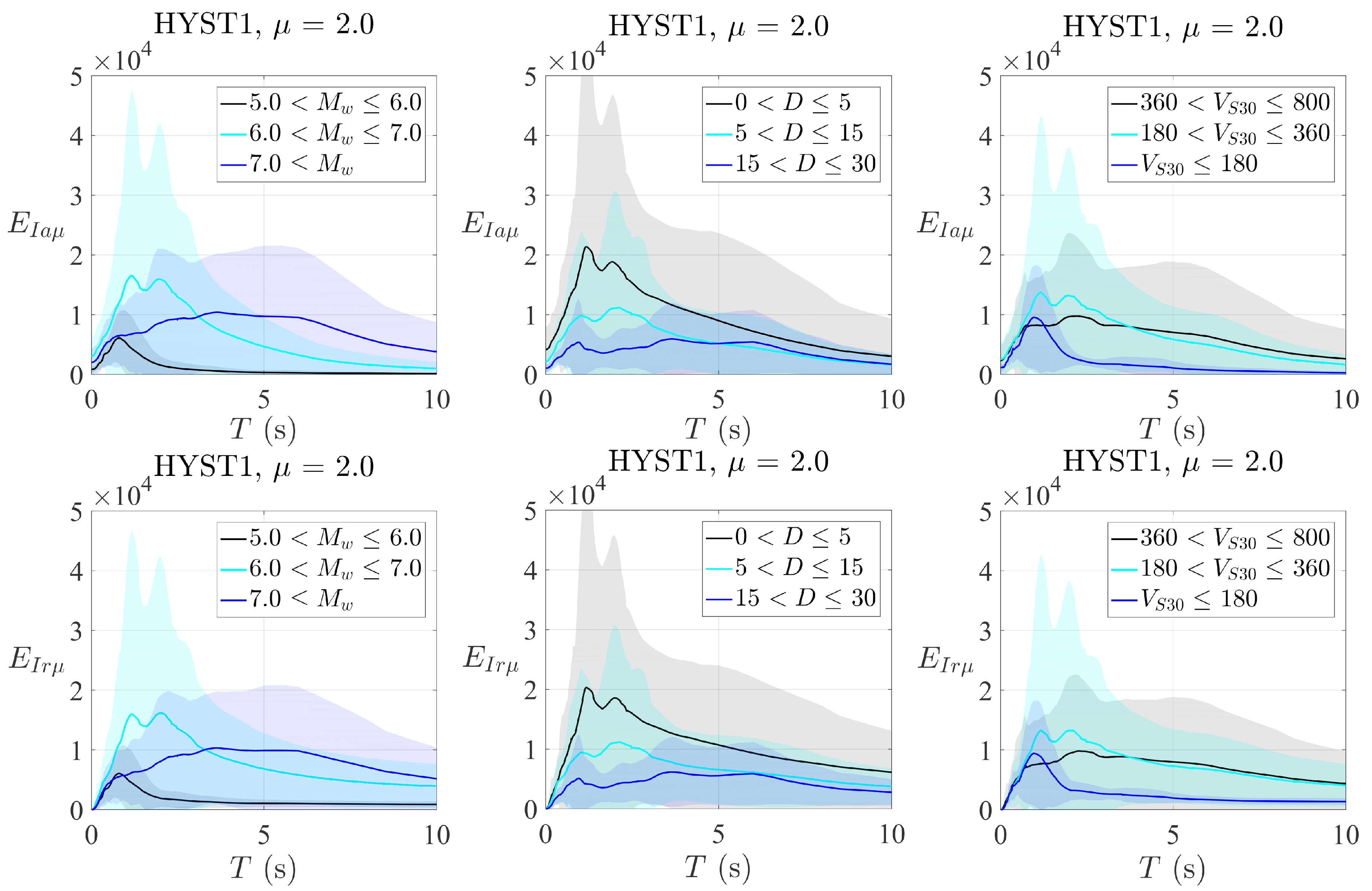
inelastic absolute E_Iaμ and relative E_Irμ input energy for the given ductility demand μ;

-

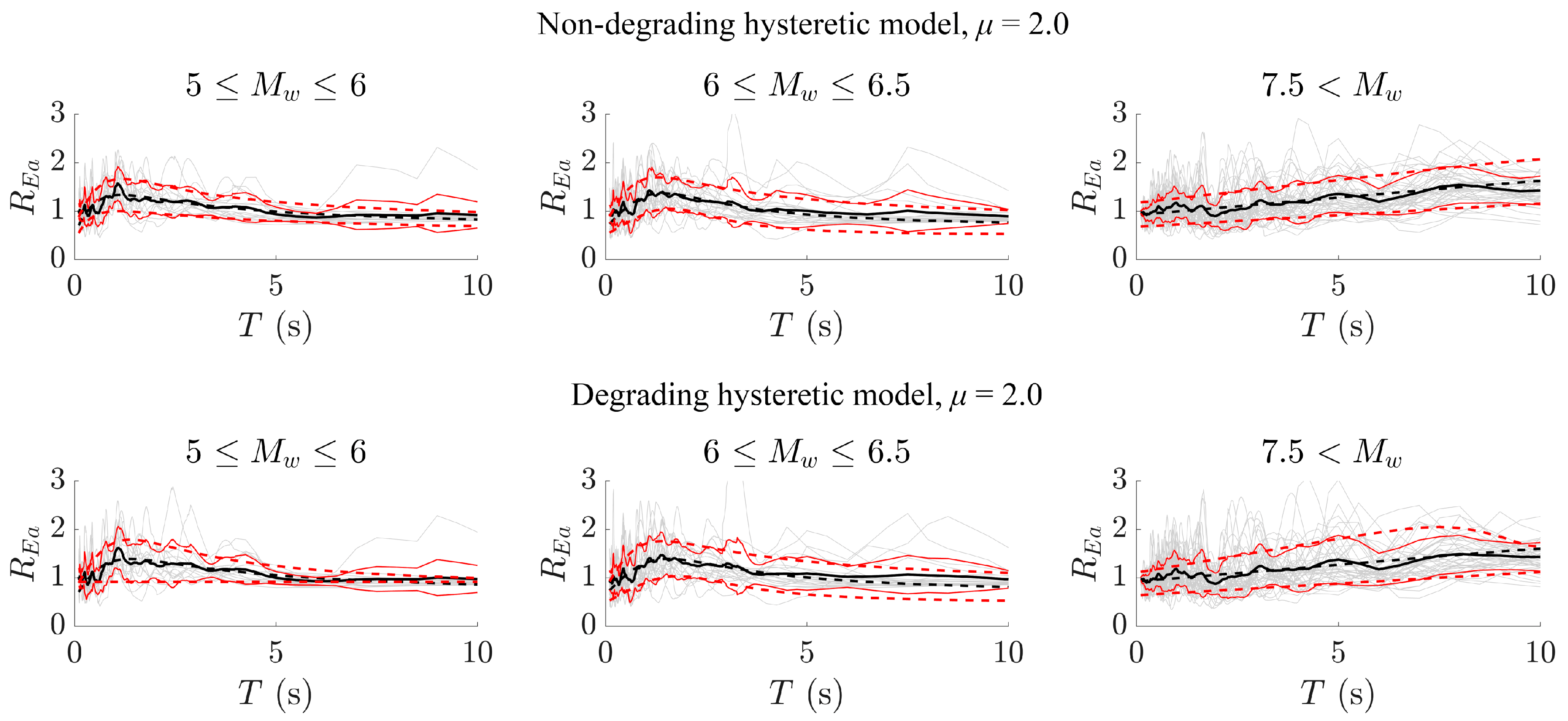
input energy reduction factors, R_Ea = E_Ia/E_Iaμ and R_Er = E_Ir/E_Irμ (i.e., the ratio between the elastic input energy and the inelastic value corresponding to a given ductility demand μ);

-

the hysteretic energy dissipation demand E_H;

-

the hysteretic energy reduction factors, R_Ha = (E_H/E_Ia)_μ and R_Hr = (E_H/E_Ir)_μ (i.e., the ratio between the hysteretic energy dissipation demand and the inelastic input energy value corresponding to a given ductility demand μ);

-

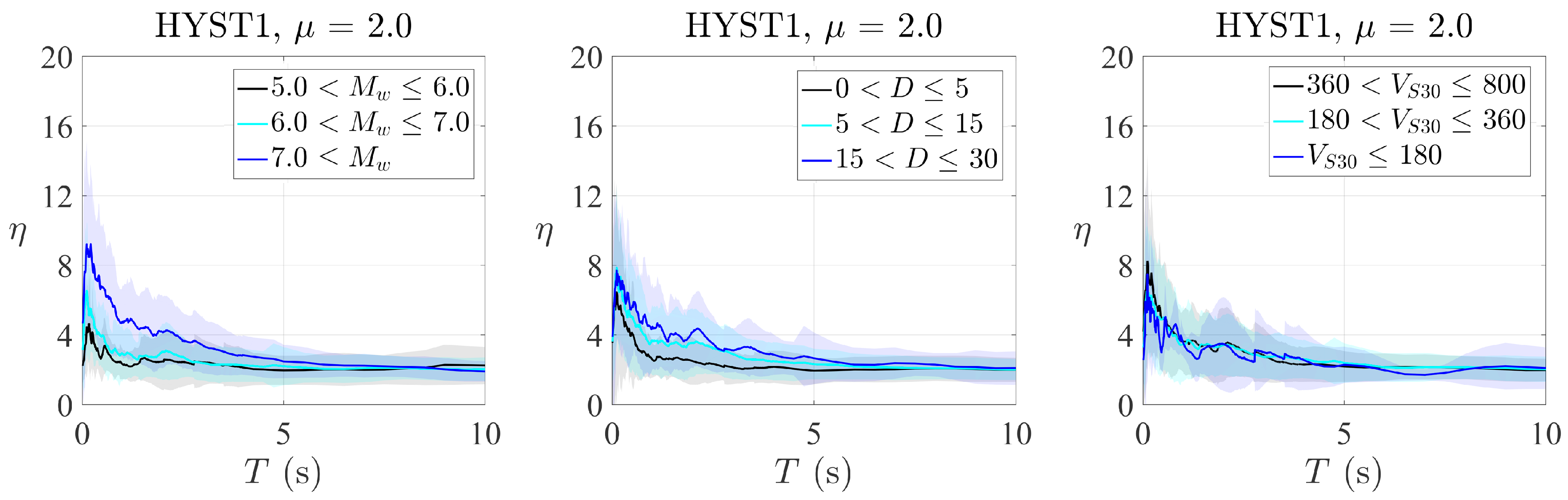
the parameter η that quantifies the plasticity level in terms of dimensionless cumulative plastic deformation ratio, i.e., η = E_H/(R_yδ_y), where R_y and δ_y are the elastic limit strength and displacement, respectively.

The influence of seismological parameters and hysteretic behavior on the spectra of these energy-related parameters is initially examined. Next, closed-form approximations are proposed for these spectra, and the numerical values of the corresponding parameters are also calibrated (with reference to both mean and standard deviation values). Overall, the objectives of this study are twofold. On one hand, it is meant to investigate the role of seismological parameters and hysteretic behavior on the seismic demand from an energy-based perspective. On the other hand, it is also intended to support the formulation of energy-based design spectra.

4. Database of Horizontal Fault-Normal Pulse-like Seismic Ground Motion Records

The dataset of horizontal fault-normal pulse-like seismic ground motions employed in the present study was prepared by collecting relevant time histories from the Engineering Strong-Motion (ESM) database, the Italian Accelerometric Archive (ITACA), the Pacific Earthquake Engineering Research Center (PEER) Ground Motion Database and the Center for Engineering Strong Motion Data (CESMD). The considered dataset is characterized by closest site-to-source distances (D_f) less than 30 km, moment magnitudes (M_w) greater than 5.0 and soil preferred shear-velocities (V_S30) between 160 m/s and 1000 m/s. It is highlighted, however, that the largest part of the selected records belonged to two soil classes only, namely B and C according to the Eurocode 8 soil classification. It is also pointed out that the maximum closest site-to-source distance within the final dataset was slightly larger than the limit distances commonly considered in similar studies, and it was meant to possibly take into account the pulse-like seismic ground motions induced by very large magnitude earthquakes. Moreover, only records with moment magnitudes larger than 5.0 were used in order to focus on the range of magnitude values that generally dictates the hazard in medium-to-high seismicity regions. The full set of values of the most relevant seismological parameters is provided in Figure 2. Herein, the pulse period (T_p) was estimated according to the methodology illustrated in [14]. As already pointed out in previous studies (see for instance [6,9,14]), it is especially highlighted that near-fault pulse-like earthquakes can exhibit very high values of T_p.

5. Sensitivity Analysis

5.1. Clustering of Seismic Records

Spectra of the selected energy-related parameters were computed and then discussed for various subsets of seismic signals having similar seismological characteristics in terms of earthquake magnitude, site-to-source distance and soil type, in such a way as to discriminate the possible influence of each of them. Details about the subsets of seismic records are provided in

Table 3. Definition of the subsets of seismic records for the sensitivity analysis (the number of records is indicated within brackets).

Moment Magnitude Mw	Closest Site-to-Source Distance Df (km)	Soil Type VS30 (m/s)
5–6 (14)	0–5 (31)	<180 (10)
6–7 (64)	5–15 (63)	180–360 (66)
>7 (49)	15–30 (24)	360–800 (51)

.

The spectra were calculated for period values T up to 10 s as follows: step of 0.01 s for T < 4 s, step of 0.025 s for 4 s < T < 5 s and step of 0.5 s for 5 s < T < 10 s. It was pointed out that the spectra were calculated for a period up to 10 s to properly account for seismic records with mid-long pulse periods (as can be observed in Figure 2). For most common practical applications, however, T < 4 s is of special interest, which is why the highest resolution for spectra value calculations was employed in this range.

5.2. Influence of Seismological Parameters

Henceforth, for the sake of conciseness, the spectra calculated for the hysteretic model HYST1 and a ductility level μ equal to 2 only were given in order to assess the influence of most common seismological parameters employed for hazard quantification in design codes, namely earthquake magnitude, site-to-source distance and soil type. It was found, however, that the main findings of this evaluation also hold true for other hysteretic models and ductility level.

In this perspective, absolute E_Iaμ and relative E_Irμ input energy are shown in Figure 3.

It can be inferred from Figure 3 that the differences between absolute and relative input energy spectra were basically negligible. In this regard, it was pointed out in [30] that relative and absolute input energies usually exhibit similar spectra in cases of forward directivity without distinctive acceleration pulses. It was also noted in [30] that the presence of a distinct acceleration pulse generates smaller or larger amplitudes in the short- and long-period ranges of the relative energy spectra, respectively, than those observed in the absolute energy spectra (i.e., the difference between relative and absolute energy becomes largest during sudden energy spikes). As seen in Figure 3, therefore, it is understood that distinctive acceleration pulses are not very common (at least within the considered database), since a large enough set of seismic records basically hides the possible differences between absolute and relative input energy. As expected, the larger the magnitude was, the larger was the period at which the peak value of the relative or absolute energy spectrum was attained. This is attributable to the fact that the peak value of the relative or absolute energy spectrum is commonly attained in the vicinity of the pulse period which, in turn, scales up when the earthquake magnitude increases [14]. Moreover, the larger is the earthquake magnitude, the longer is the period range for which relative or absolute energy spectral values are close to the peak. Figure 3 also confirms that higher energy demands are expected as the site-to-source distance becomes shorter and shorter, whereas it highlights that input energy spectra also become significantly flatter when the distance increases. Furthermore, Figure 3 suggests that absolute and relative input energy spectra are influenced by the soil type for rather low values of V_S30 only, namely less than 180 m/s. Otherwise, no significant effects are produced, since the mean spectra for V_S30 larger than 180 m/s are very close to each other and almost overlap for period values larger than 4 s. This evidence, however, is not conclusive and might be affected by statistical distortion, since the number of seismic records with V_S30 less than 180 m/s is low and much less than the number of those available for V_S30 between 180 m/s and 360 m/s or between 360 m/s and 800 m/s.

It was also convenient to investigate the input energy reduction factors R_Ea and R_Er for a given ductility demand μ. To this end, the spectra related to R_Ea only are shown in Figure 4 because they have similar results as those carried out for R_Er. It can be noted from Figure 4 that the mean spectra of the absolute input energy reduction factor R_Ea in terms of earthquake magnitude and site-to-source distance were not too far each other for period values less than 4 s. On the other hand, mean spectra of the absolute input energy reduction factor in terms of soil type were closer to each other for almost the whole range of period values.

The analysis of the hysteretic energy dissipation demand spectra E_H provided no enlightening new evidence about the role of seismological parameters on the energy demand with respect to the conclusions already drawn from the analysis of absolute E_Iaμ and relative E_Irμ input energy spectra, as can be concluded by comparing Figure 3 and Figure 5.

It was also opportune to investigate the hysteretic energy reduction factors R_Ha and R_Hr for a given ductility demand μ. Assuming the hysteretic energy reduction factor R_Ha as a reference parameter, Figure 6 shows that it was strongly affected by the earthquake magnitude and to a lesser extent by soil type, whereas the site-to-source distance did not produce very large effects. Specifically, the increment of the earthquake magnitude caused a shifting on the right of the period at which the peak of the hysteretic energy reduction factor was attained. In addition, the larger the earthquake magnitude was, the lower was the slope of the post-peak branch of the hysteretic energy reduction factor R_Ha spectrum. Note, however, that the peak value of the hysteretic energy reduction factor R_Ha spectrum did not seem much affected by the earthquake magnitude, and its variability decreased when the earthquake magnitude increased. Regarding the influence of the soil type, it appeared evident for rather low values of V_S30 only, but it might be possible that this evidence could have been corrupted by the low number of seismic records available for V_S30 less than 180 m/s.

Finally, the spectra for the cumulative plastic deformation ratio η are reported in Figure 7. The analysis of this energy-related parameter was especially important because the hysteretic energy demand E_H alone cannot provide a proper assessment of the structural behavior, particularly for reinforced concrete structures. In fact, the hysteretic energy associated with structural systems having small strength and undergoing a large cyclic response can be similar to that experienced by structural systems having large strength but undergoing a small cyclic response.

It is evident that the cumulative plastic deformation ratio η was less affected by seismological parameters with respect to the hysteretic energy demand E_H. As a matter of fact, the mean spectra of the cumulative plastic deformation ratio η differed significantly only for very large earthquake magnitude values and period values less than 4 s.

5.3. Influence of Hysteretic Model and Ductility Level

From a qualitative standpoint, the shape of the energy-related spectra and their sensitivity with respect to the main seismological parameters (i.e., earthquake magnitude, site-to-source distance and soil type) was not markedly affected by the hysteretic model and its constitutive model parameters. From a quantitative standpoint, however, significant differences could be observed for some energy-related parameters. In particular, small differences were observed when comparing mean spectra of absolute E_Iaμ and relative E_Irμ input energy as well as those for input energy reduction factors R_Ea and R_Er and hysteretic energy dissipation demand E_H. The observed differences became larger and larger for increasing values of the ductility level μ. On the other hand, the spectra of the hysteretic energy reduction factors R_Ha and R_Hr as well as those for the cumulative plastic deformation ratio η were affected to a rather larger extent by hysteretic behavior and/or the ductility level μ (see Figure 8 and Figure 9). Particularly, these plots emphasized that large differences can arise in the spectra of the hysteretic energy reduction factor and the cumulative plastic deformation ratio if non-degrading systems (i.e., EPP and HYST1) or degrading ones (i.e., HYST2, HYST3, HSYT4 and HYST5) are compared. These differences were also amplified for increasing values of the ductility level.

As already pointed out in [28], structural systems experiencing stiffness and strength degradation do not necessarily require high yielding strengths for a given ductility value. The fact that the force imposed on systems with degrading behavior is less demanding than that imposed on elastoplastic systems can be explained by considering that the response of the former features a larger number of hysteretic cycles at smaller amplitude. Elastoplastic systems have greater chances of drifting and hence require more strength capacity than the degrading ones to limit the deformation up to the prescribed damage level.

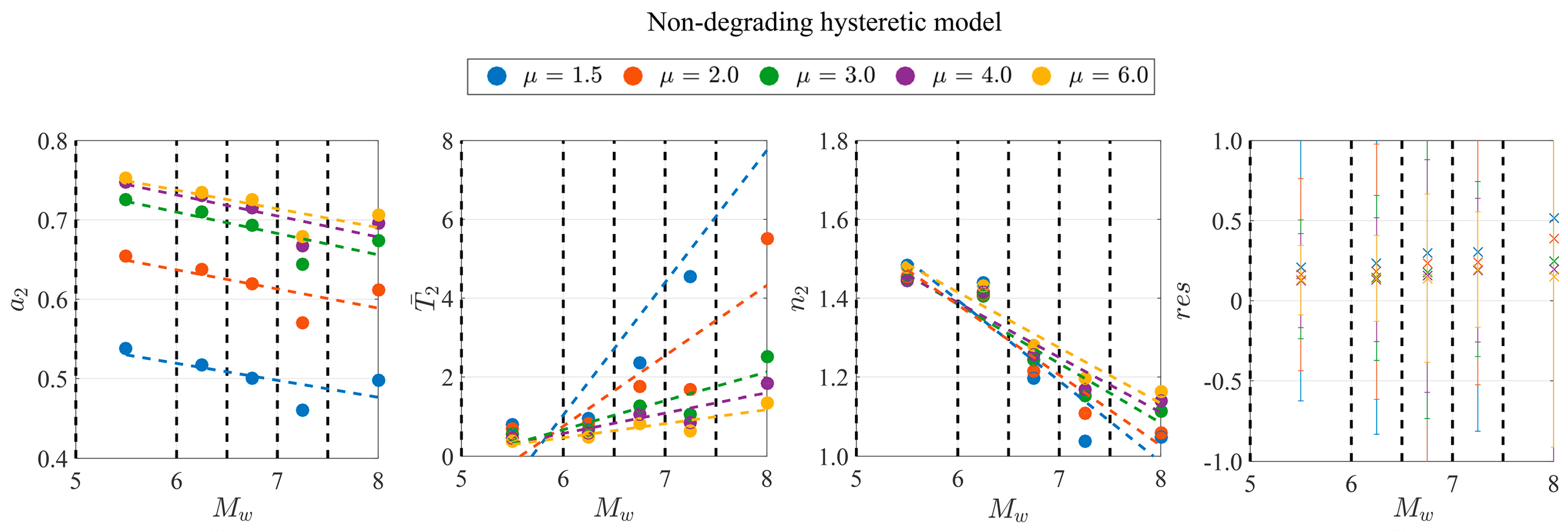
6. Closed-Form Approximation of Energy-Related Spectra

Closed-form approximations for the spectra of relevant energy-related parameters are now proposed. Particularly, the following functional form is proposed to approximate the spectra of input energy and input energy reduction factor:

$${ℱ}_1=b_1+a_1\left(\frac{T}{{\overline{T}}_1}\right)\left[\frac{n_1}{n_1-1+{\left(\frac{T}{{\overline{T}}_1}\right)}^{n_1}}\right]$$

(2)

On the other hand, it is proposed to approximate the spectra of the hysteretic energy reduction factor using the following functional form:

$${ℱ}_2=a_2\left(\frac{T}{{\overline{T}}_2}\right)\left[\frac{n_2}{n_2-1+{\left(\frac{T}{{\overline{T}}_2}\right)}^{n_2}}\right]$$

(3)

Finally, the spectra of the cumulative plastic deformation ratio is approximated using a modified version of the functional form employed in [28]:

$${ℱ}_3={\left[a_3+\left(\frac{1}{\mu }-1\right)e^{-b_3 T^{c_3} {\mu }^{-n_3}}\right]}^{-1}.$$

(4)

These closed-form approximations involve some constants, the numerical values of which are determined through a regression analysis intended to minimize the sum of squared residuals. In order to provide an effective support for the development of energy-based design spectra, mean and standard deviation values were considered in the regression analysis. Additionally, there was also the need to look for a compromise between simplicity and accuracy. To this end, several preliminary regressions analyses were conducted by employing different combinations of the considered seismological parameters and hysteretic behaviors. In so doing, the best compromise was found by considering the earthquake magnitude only together with the type of hysteretic behavior (i.e., non-degrading or degrading) and the associated ductility level. This agreed with the outcomes of the sensitivity analysis. In fact, the earthquake magnitude was found to be the most influent parameter, since it directly affected both pulse period and maximum seismic demand value. The influence of soil type was found to be rather modest, perhaps because of a statistical distortion in the available database, since selected records belong to classes B and C according to the Eurocode 8 soil classification. Since near-fault earthquakes were herein considered, it seems reasonable that the less influential seismological parameter was the site-to-source distance. Furthermore, the sensitivity analysis highlighted that large differences in the spectral values can occur when comparing non-degrading and degrading behaviors (regardless of the specific hysteretic model, at least for typical behaviors observed in ordinary civil constructions made of steel, masonry or concrete) for different ductility levels.

After parameters calibration, it was found that the proposed closed-form approximations provided very good predictions of the energy demand values (see, for instance, the results in Figure 10, Figure 11, Figure 12 and Figure 13). It was pointed out that the regression analysis in Figure 11 and Figure 13 was valid for T > 0.1 s, whereas in general, a better accuracy was achieved for T ≤ 4 s. The greater accuracy for low-mid period values did not depend on the regression model or the parameter calibration. Conversely, this was because there were more spectral values at low period values, whereas just a few data points were available for mid-long period values. This, in turn, implied that the regression analysis was forced to achieve a better accuracy level for low–mid period values rather than for mid–long ones. This is a desired output, since low period values are of interest for most ordinary structural applications.

An attempt was made to correlate the constants involved in Equations (2)–(4) with the earthquake magnitude. In doing so, satisfactory closed-form correlations were obtained for the constants involved in the regression formula of the spectra of the hysteretic energy reduction factor (see Figure 14 and Figure 15). For the remaining energy parameters, no closed-form correlations were found between the constants of the regression formula and the earthquake magnitude. All details about the numerical values of these constants are given in the Appendix A and Supplementary Materials.

7. Conclusions

The analysis of structures under seismic loads in terms of energy provides an alternative standpoint to well-established strategies based on force and displacements. The usefulness of an energy-based approach in earthquake engineering is especially appropriate for structures and infrastructures in near-fault areas, because seismic ground motions here recorded typically exhibit a pulse-like waveform in the velocity component. It is evident, however, that the implementation of an energy-based approach in the assessment and design of structures subjected to near-fault pulse-like earthquakes calls for the definition of relevant design demand spectra. In this perspective, the present work is a further step forward in the potential practical implementation of energy principles in earthquake engineering. First, it explained the role of seismological parameters and hysteretic behavior on the energy demand on inelastic systems. Moreover, it proposed closed-form approximations for relevant energy-based spectra (with reference to mean and standard deviation values), the parameters of which are given as functions of earthquake magnitude, type of hysteretic behavior (i.e., non-degrading or degrading) and ductility level.

References

1. Archuleta, R.J.; Hartzell, S.H. Effects of fault finiteness on near-source ground motion. Bull. Seism. Soc. Am. 1981, 71, 939–957. [Google Scholar]
2. Somerville, P.G.; Graves, R.W. Conditions that give rise to unusually large long period ground motions. In Proceedings of the Seminar on Seismic Isolation, Passive Energy Dissipation and Active Control, Applied Technology Council, San Francisco, CA, USA, 11–12 March 1993; pp. 83–94. [Google Scholar]
3. Hall, J.F.; Heaton, T.H.; Halling, M.W.; Wald, D.J. Near-source ground motion and its effects on flexible buildings. Earthq. Spectra 1995, 11, 569–605. [Google Scholar] [CrossRef]
4. Somerville, P.G.; Smith, N.F.; Graves, R.W.; Abrahamson, N.A. Modification of empirical strong ground motion attenuation relations to include the amplitude and duration effects of rupture directivity. Seism. Res. Lett. 1997, 68, 199–222. [Google Scholar] [CrossRef]
5. Menun, C.; Fu, Q. An analytical model for near-fault ground motions and the response of SDOF systems. In Proceedings of the 7th U.S. National Conference on Earthquake Engineering, Boston, MA, USA, 21–25 July 2002. [Google Scholar]
6. Mavroeidis, G.P.; Papageorgiou, A.S. A mathematical representation of near-fault ground motions. Bull. Seism. Soc. Am. 2003, 93, 1099–1131. [Google Scholar] [CrossRef]
7. Bray, J.D.; Rodriguez-Marek, A. Characterization of forward-directivity ground motions in the near-fault region. Soil Dyn. Earthq. Eng. 2004, 24, 815–828. [Google Scholar] [CrossRef]
8. Mollaioli, F.; Bruno, S.; Decanini, L.D.; Panza, G.F. Characterization of the dynamic response of structures to damaging pulse-type near-fault ground motions. Meccanica 2006, 41, 23–46. [Google Scholar] [CrossRef] [Green Version]
9. Baker, J.W. Quantitative classification of near-fault ground motions using wavelet analysis. Bull. Seism. Soc. Am. 2007, 97, 1486–1501. [Google Scholar] [CrossRef]
10. Lu, Y.; Panagiotou, M. Characterization and representation of near-fault ground motions using cumulative pulse extraction with wavelet analysis. Bull. Seism. Soc. Am. 2013, 104, 410–426. [Google Scholar] [CrossRef]
11. Mukhopadhyay, S.; Gupta, V.K. Directivity pulses in near-fault ground motions—I: Identification, extraction and modeling. Soil Dyn. Earthq. Eng. 2013, 50, 1–15. [Google Scholar] [CrossRef]
12. Chang, Z.; Sun, X.; Zhai, C.; Zhao, J.X.; Xie, L. An improved energy-based approach for selecting pulse-like ground motions. Earthq. Eng. Struct. Dyn. 2016, 45, 2405–2411. [Google Scholar] [CrossRef]
13. Dabaghi, M.; Der Kiureghian, A. Simulation of orthogonal horizontal components of near-fault ground motion for specified earthquake source and site characteristics. Earthq. Eng. Struct. Dyn. 2018, 47, 1369–1393. [Google Scholar] [CrossRef]
14. Quaranta, G.; Mollaioli, F. Analysis of near-fault pulse-like seismic signals through Variational Mode Decomposition technique. Eng. Struct. 2019, 193, 121–135. [Google Scholar] [CrossRef]
15. Makris, N. Rigidity-plasticity-viscosity: Can electrorheological dampers protect base-isolated structures from near-source ground motions? Earthq. Eng. Struct. Dyn. 1997, 26, 571–591. [Google Scholar] [CrossRef]
16. Alavi, B.; Krawinkler, H. Behavior of moment-resisting frame structures subjected to near-fault ground motions. Earthq. Eng. Struct. Dyn. 2004, 33, 687–706. [Google Scholar] [CrossRef]
17. Rupakhety, R.; Sigbjörnsson, R. Can simple pulses adequately represent near-fault ground motions? J. Earthq. Eng. 2011, 15, 1260–1272. [Google Scholar] [CrossRef]
18. Alonso-Rodríguez, A.; Miranda, E. Assessment of building behavior under near-fault pulse-like ground motions through simplified models. Soil Dyn. Earthq. Eng. 2015, 79, 47–58. [Google Scholar] [CrossRef]
19. Mazza, M. Effects of near-fault ground motions on the nonlinear behaviour of reinforced concrete framed buildings. Earthq. Sci. 2015, 28, 285–302. [Google Scholar] [CrossRef] [Green Version]
20. Quaranta, G.; Mollaioli, F.; Monti, G. Effectiveness of design procedures for linear TMD installed on inelastic structures under pulse-like ground motion. Earthq. Struct. 2016, 10, 239–260. [Google Scholar] [CrossRef]
21. MacRae, G.A.; Morrow, D.W.; Roeder, C.W. Near-fault ground motion effects on simple structures. J. Struct. Eng. 2001, 127, 996–1004. [Google Scholar] [CrossRef]
22. Cuesta, I.; Aschheim, M.A. Inelastic response spectra using conventional and pulse R-factors. J. Struct. Eng. 2001, 127, 1013–1020. [Google Scholar] [CrossRef]
23. Mavroeidis, G.P.; Dong, G.; Papageorgiou, A.S. Near-fault ground motions, and the response of elastic and inelastic single-degree-of-freedom (SDOF) systems. Earthq. Eng. Struct. Dyn. 2004, 33, 1023–1049. [Google Scholar] [CrossRef]
24. Kalkan, E.; Kunnath, S.K. Effects of fling-step and forward directivity on the seismic response of buildings. Earthq. Spectra 2006, 22, 367–390. [Google Scholar] [CrossRef]
25. Tong, M.; Rzhevsky, V.; Junwu, D.; Lee, G.C.; Jincheng, Q.; Xiaozhai, Q. Near-fault ground motion with prominent acceleration pulses: Pulse characteristics and ductility demand. Earthq. Eng. Eng. Vib. 2007, 6, 215–223. [Google Scholar] [CrossRef]
26. Hatzigeorgiou, G.D.; Pnevmatikos, N.G. Maximum damping forces for structures with viscous dampers under near-source earthquakes. Eng. Struct. 2014, 68, 1–13. [Google Scholar] [CrossRef]
27. Makris, N.; Black, C. Evaluation of peak ground velocity as a good intensity measure for near-source ground motions. J. Eng. Mech. 2004, 130, 1032–1044. [Google Scholar] [CrossRef]
28. Mollaioli, F.; Bruno, S. Influence of site effects on inelastic displacement ratios for SDOF and MDOF systems. Comput. Math. Appl. 2008, 55, 184–207. [Google Scholar] [CrossRef] [Green Version]
29. Donaire-Ávila, J.; Benavent-Climent, A.; Lucchini, A.; Mollaioli, F. Energy-based seismic design methodology: A preliminary approach. In Proceedings of the 16th World Conference on Earthquake Engineering, 16WCEE 2017, Paper N° 2106. Santiago, Chile, 9–13 January 2017. [Google Scholar]
30. Kalkan, E.; Kunnath, S.K. Relevance of absolute and relative energy content in seismic evaluation of structures. Adv. Struct. Eng. 2008, 11, 17–34. [Google Scholar] [CrossRef]
Figure 1. Displacement u—restoring force R response of the analyzed hysteretic single-degree-of-freedom (SDOF) systems (Table 1) for the considered set of model parameter values (Table 2).
Applsci 10 07578 g001
Figure 2. Variability of moment magnitude Mw, closest site-to-source distance Df and soil preferred shear-velocities VS30 as function of the pulse period Tp within the considered dataset.
Applsci 10 07578 g002
Figure 3. Spectra of the absolute EIaμ and relative EIrμ input energy for the hysteretic model HYST1 and ductility level μ equal to 2 considering different subsets of seismic records (filled area: envelope of the spectra; solid line: mean spectrum).
Applsci 10 07578 g003
Figure 4. Spectra of the absolute input energy reduction factor REa for the hysteretic model HYST1 and ductility level μ equal to 2 considering different subsets of seismic records (filled area: envelope of the spectra; solid line: mean spectrum).
Applsci 10 07578 g004
Figure 5. Spectra of the hysteretic energy dissipation demand EH for the hysteretic model HYST1 and ductility level μ equal to 2 considering different subsets of seismic records (filled area: envelope of the spectra; solid line: mean spectrum).
Applsci 10 07578 g005
Figure 6. Spectra of the hysteretic energy reduction factor RHa for the hysteretic model HYST1 and ductility level μ equal to 2 considering different subsets of seismic records (filled area: envelope of the spectra; solid line: mean spectrum).
Applsci 10 07578 g006
Figure 7. Spectra of the cumulative plastic deformation ratio η for the hysteretic model HYST1 and ductility level μ equal to 2 considering different subsets of seismic records (filled area: envelope of the spectra; solid line: mean spectrum).
Applsci 10 07578 g007
Figure 8. Influence of the hysteretic model on the spectra of absolute input energy reduction factor REa for a ductility level μ equal to 2 (filled area: envelope of the spectra; solid line: mean spectrum).
Applsci 10 07578 g008
Figure 9. Influence of the hysteretic model on the spectra of elastic limit strength Ry and cumulative plastic deformation ratio η for a ductility level μ equal to 4 (filled area: envelope of the spectra; solid line: mean spectrum).
Applsci 10 07578 g009
Figure 10. Comparison between calculated absolute input elastic energy EIa spectra (mean and mean plus/minus one standard deviation) and proposed approximation (thin solid line: single spectrum; thick solid line: calculated spectrum; thick dashed line: proposed approximation).
Applsci 10 07578 g010
Figure 11. Comparison between calculated absolute input energy reduction factor REa spectra (mean and mean plus/minus one standard deviation) and proposed approximation (thin solid line: single spectrum; thick solid line: calculated spectrum; thick dashed line: proposed approximation).
Applsci 10 07578 g011
Figure 12. Comparison between calculated hysteretic energy reduction factor RHa spectra (mean and mean plus/minus one standard deviation) and proposed approximation (thin solid line: single spectrum; thick solid line: calculated spectrum; thick dashed line: proposed approximation).
Applsci 10 07578 g012
Figure 13. Comparison between calculated cumulative plastic deformation ratio η spectra (mean and mean ± one standard deviation) and proposed approximation (thin solid line: single spectrum; thick solid line: calculated spectrum; thick dashed line: proposed approximation).
Applsci 10 07578 g013
Figure 14. Constants involved in the regression analysis of the mean spectra of the hysteretic energy reduction factor RHa for hysteretic non-degrading behaviors (dots: regression results; line: proposed closed-form relationship), together with the regression error chart.
Applsci 10 07578 g014
Figure 15. Constants involved in the regression analysis of the mean spectra of the hysteretic energy reduction factor RHa for hysteretic degrading behaviors (dots: regression results; line: proposed closed-form relationship), together with the regression error chart.
Applsci 10 07578 g015