1. Introduction
River-based hydrokinetic turbines represent a clean and ecological way to harness the water energy of streams and could have a significant contribution in the future to the renewable energy sector due to their potential in a variety of river crossing areas around the world. However, hydrokinetic turbines are still in the early stage of development and various optimized solutions can be identified in the literature and in specific projects. The main drawback of such devices is their sensitivity to water flow rates and rotational speed variations because the rotor is placed directly into the water current. In the field of hydrokinetic turbines, some improvements were made recently on the rotor design, including blade optimization and the use of various shroud shapes that aimed to increase the power coefficients. Different studies and research have focused on identifying the most suitable technical solutions and operating conditions that lead to an increased power extraction. The authors in [
1] numerically investigated a patented new concept of 1 kW ducted isokinetic turbine with improved axial velocity given by two joined concentric runners. Some studies [
2] have assessed the blade chord length influence on the efficiency of a shrouded horizontal axis hydrokinetic turbine, while others [
3] have focused on identifying a power prediction method for a given velocity and a range of hydrokinetic turbines by using experimental data for different rotors with similar geometry. A power prediction curve is obtained by adapting the power coefficient variation with tip speed ratio. Other studies have analyzed experimentally [
4] or both numerically and experimentally [
5] the development of ducted/shrouded turbines, also called diffuser-augmented turbines, aiming to assess the increased power output. In [
6], the operation range of a kinetic turbine (marine currents turbine) was experimentally investigated in order to avoid cavitation. By performing tests under different hydrodynamic conditions in a cavitation tunnel and a towing tank, the authors determined the power and thrust characteristics for a range of rpm, flow speed, pitch angles, and immersion depth for the operation of single and twin rotors. The best performance of the turbine was obtained for tip speed ratios between 5 and 7 and hub pitch angles of approximately 20°.
Besides assessing the interference between rotors and areas of cavitation inception, the research also identified that a reduced immersion depth leads to a low extracted power. Since harnessing the kinetic energy of water is the subject of numerous studies that analyze different scientific, technological, and economic aspects related to kinetic turbines use, reviews focusing on the current development and challenges of this technology have been published [
7], as well as study cases for certain countries [
8,
9] or areas [
10], characterized by specific available flow velocities. For example, the steps for achieving a kinetic turbine suitable for ensuring the power of remote communities are presented in [
10], giving details regarding turbine sizing, blade design, and construction.
An electronic power converter and control system can also be used to increase the power output. The majority of solutions aiming maximum power point tracking (MPPT) optimization are focused on wind turbines and photovoltaic (PV) power plants due to their spread and accessibility. Micro-hydropower plants can also benefit from the optimization systems mentioned in the literature [
11,
12,
13,
14,
15,
16,
17,
18,
19]. The controllers used for this purpose can be classified into three main control methods, namely, tip speed ratio (TSR) control, power signal feedback (PSF) control, and hill-climb search (HCS) control. The proposed model for MPPT algorithm uses a hill-climb search (HCS) method based on perturbation and observation (P&O) of the self-regulating system, implemented in the simulation. Because the velocity of flowing water is variable and unpredictable, developing reliable methods to track the optimal operation point of the hydrokinetic turbines is necessary in order to extract the maximum available power at a certain time. In [
11], MATLAB software was used to obtain real-time point to point discrete MPPT simulation applicable to the wind energy system, which uses a permanent magnet synchronous generator (PMSG). The system model has a three-phase rectifier and a buck converter with its input ratio controlled by a PWM (pulse width modulation) signal from the maximum power point controller. In [
12], an MPPT algorithm that uses a neural network compensator for the uncertainties in wind turbine generation systems is proposed. A proportional integral (PI) controller determines the duty cycle of the DC/DC converter and the parameters are determined by a genetic algorithm. By imposing certain variations for the wind speed and air density, the power coefficient is kept approximately at its maximum value. Other studies, such as [
13], focused on implementing the MPPT algorithm to hybrid solar–wind systems, aiming at extracting the maximum power (tracked by a boost converter) from both sources. A single modified P&O control algorithm that reduces the complexity of the overall system was applied and compared with conventional P&O algorithm. In [
14], the modeling and simulation results for a hybrid wind solar energy system using MPPT were presented. The proposed system presented power control strategies of a grid-connected hybrid generation system with versatile power transfer. Two MPPT control methods (TSR and optimal torque, OT) are used in [
15] for a 1.5 MW wind turbine under different wind conditions: 6, 8, and 10 m/s. Even if the TSR method has some advantages over the commercial OT method, both have limitations. For example, the TSR controller gives better results than the OT controller in terms of optimal TSR tracking, power production performance, and faster response but has significant variations of rotor speed and power output that induce large loads for the wind turbine components. Thus, the algorithm could be useful for large wind turbine designers in deciding whether to maximize power output or optimize component loads. In [
16], the P&O method is applied to a 3 kW wind turbine considering various electrical loads and wind velocities. An increase in power output was found for different operating conditions, with the MPPT algorithm providing the best results for a load of 200 Ω and 6.5 m/s wind velocity and proving its efficiency in enhancing the performance of wind turbine systems. In [
17], a HCS type MPPT algorithm consisting of PMSG, uncontrolled rectifier, and DC boost converter was applied for a hydrokinetic turbine. A PI controller was used for capturing the maximum power output of the system. Thus, the modified algorithm improved the fixed step HCS algorithm by reducing the oscillation at the steady-state condition. The variation of water velocity from 0.5 m/s to 2 m/s was considered and the results provided by the two algorithms (simple HCS and modified HCS along with PI) were compared. It was found that the second approach provided better results, with the hydrokinetic system harnessing more power. In [
18], an analysis of different expert control systems applied in MPPT of wind turbines was performed. The conclusion of the study was that the contribution of an expert system based on neural network, fuzzy logic control, or intelligent search algorithms improved the non-linearity of the variables of a system. Another approach is reported in [
19], consisting of a novel maximum power tracking strategy for wind turbine systems based on a hybrid wind velocity forecasting algorithm. In the controlling strategy, to optimize the output power, the authors proposed a state feedback control technique to achieve the rotor flux and rotor speed tracking purpose based on the MPPT algorithm verified by simulation.
Considering the benefits reported in literature when using MPPT control, it became obvious that it is possible to successfully apply this technique to hydrokinetic turbines. The algorithm applied to the hydrokinetic turbine considered in the present study is not different to the ones applied to wind turbines. Basically, an algorithm that has proven its efficiency in other wind turbine research can be also applied to kinetic turbines. The operating principle is similar for variable speed wind turbines and hydrokinetic turbines. Thus, an MPPT algorithm applied to wind turbines can be considered as the primary reference for efficiency improvement in this field.
The challenge is to instantaneously adapt the control system to specific parameters of the hydrokinetic turbine so that the maximum available power could be extracted. Moreover, the power control system has to track the turbine behavior, permanently adjusting the load according to water velocity variation. Another important function of the controller is to ensure optimum conditions for turning the rotor again after a complete stop. This can be achieved by load disconnection until proper voltage is reached. For permanent magnet synchronous generators, the only method applicable for achieving power regulation is the load adjustment.
The main objective of this paper is to design a power converter of the hydrokinetic power system in order to extract the maximum power from the flowing water. When the water velocity is high enough, a net positive power is produced by the hydrokinetic system. For certain characteristics of the hydrokinetic turbine, there is just one optimal operation point producing the maximum power for each tip speed ratio; the optimal operation point is determined by the water velocity and shaft rotational speed. Since the water velocity cannot be controlled, only the rotor speed can be adjusted to achieve the maximum power by changing the load. Therefore, the appropriate power conversion algorithm and rotor speed controller are the key components with significant impact on system efficiency [
20]. For wind and water turbines, similar MPPT algorithms can be used. Different types of control systems can be implemented, depending on the required application, aiming to follow as closely as possible the ideal curve of the electric generator for extracting the maximum power.
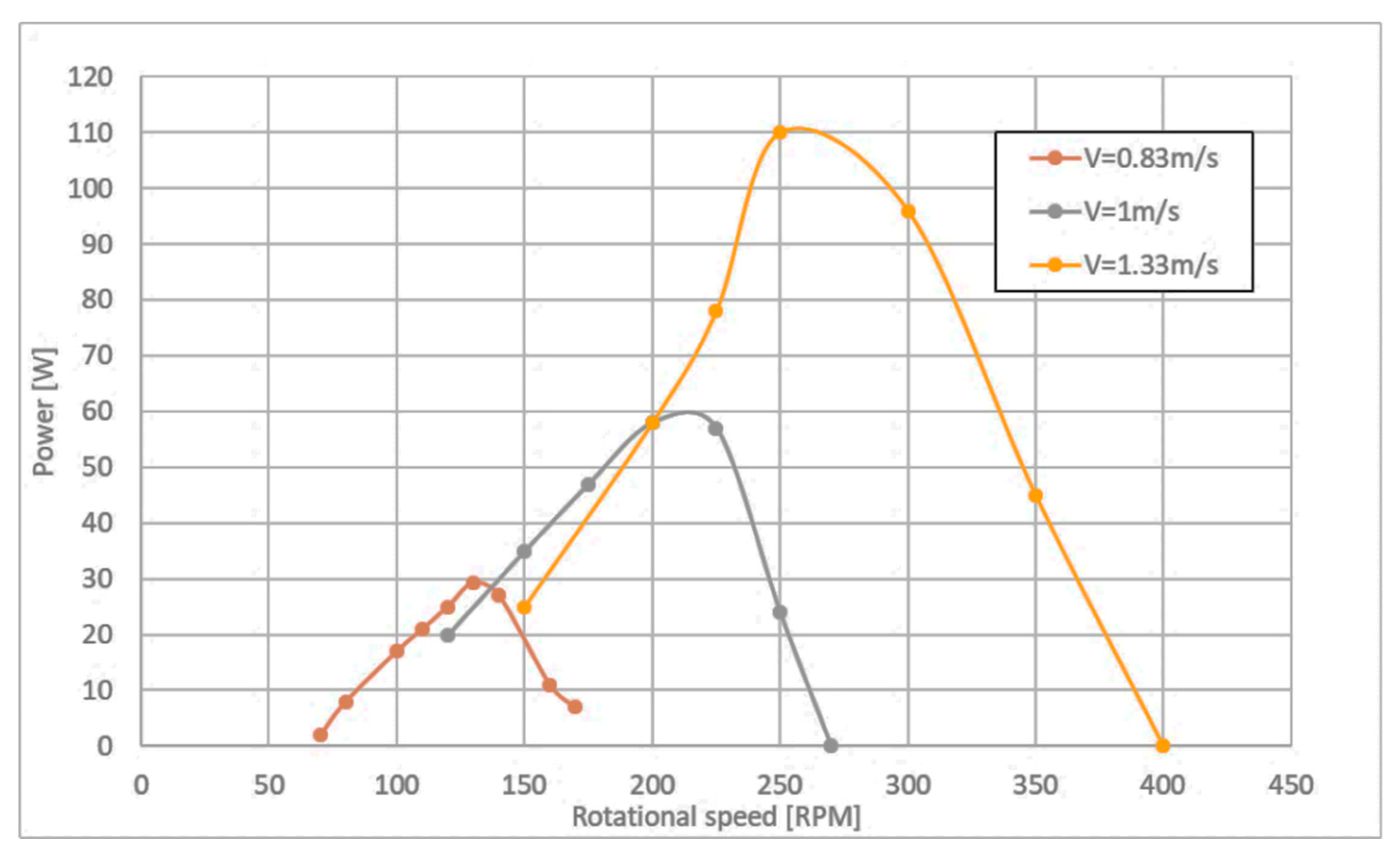
The variation of the power curves at different water velocities for a shrouded hydrokinetic turbine tested in real operating conditions during previous research [
21] is shown in
Figure 1. The investigated rotor had four Gottingen 450 blades with a diameter of 0.5 m.
The parameters of the rotor and electric generator of this hydrokinetic turbine were used as input data for the MPPT algorithm.
The novelty of the research is the implementation within the MPPT system of a DC/DC buck converter that controls the voltage applied to a certain load. This improvement is necessary for ensuring an adequate voltage in case the system is provided with a battery that requires a narrow range of voltage applied to the battery management system (BMS). For battery charging, the constant current–constant voltage (CC-CV) method was used. This method involves charging the battery at a constant current until the voltage reaches a certain threshold (depending on the battery type); then, the voltage is maintained constant and the current is adjusted until the battery is fully charged. Furthermore, the DC/DC buck converter allows for precise control of the voltage applied to the load; this aspect is very important when charging a battery because an increased voltage can damage it.
The paper is structured in three main sections. The first one describes the design of the MPPT algorithm and also the design of the two converters. To test the algorithm, we developed mathematical models for the converters, which were used in a simulation to test the validity of the control system. In the second section, the results of the simulation under different operating conditions are presented and discussed. The last section of the paper presents the conclusions of the work as well as future research directions aimed at improving the model, namely, including a battery model for the load.
2. Design of the MPPT Control Algorithm
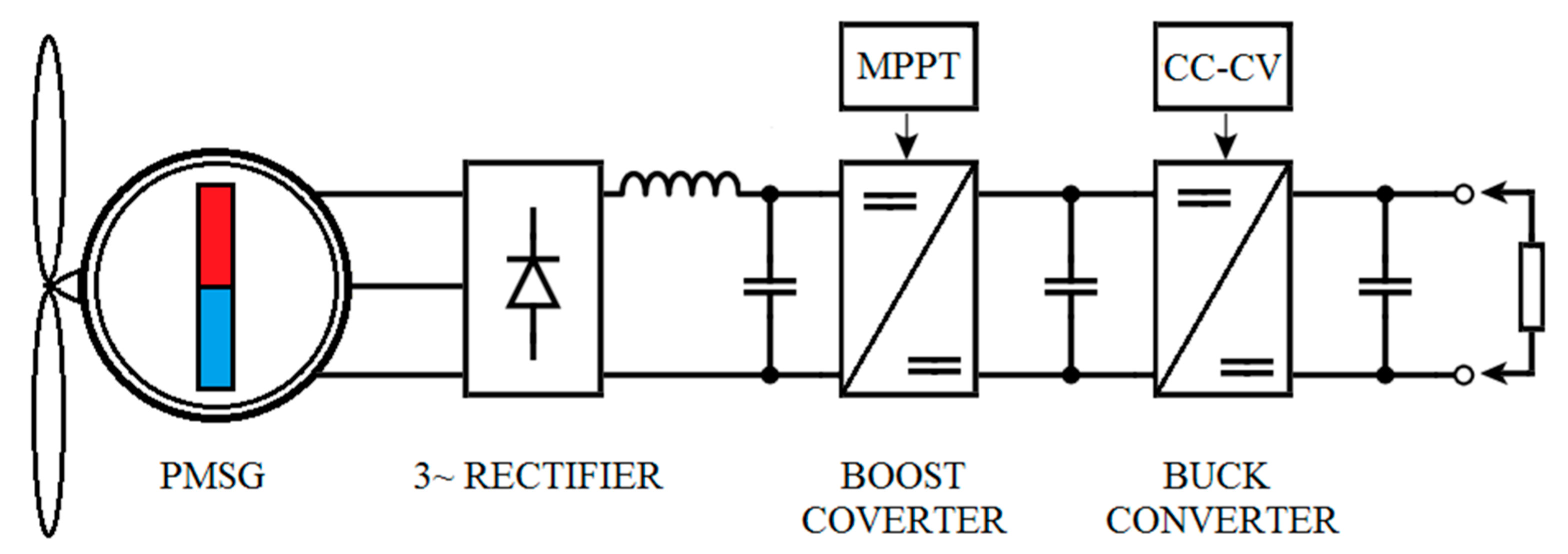
The proposed system consists of a permanent magnet three-phase generator connected to the hydrokinetic turbine, a three phase uncontrolled rectifier, a DC boost converter with MPPT control to extract maximum available power, and a buck converter with CC-CV control to impose the desired voltage and current on the load. A simulation was carried out in order to test the MPPT algorithm. The block diagram is presented in
Figure 2.
In order to test the MPPT algorithm, we built the individual blocks on the basis of the corresponding equations of each component. The hydrokinetic turbine is modeled on the basis of the following equation:
where
—water density (kg/m3);
—turbine radius (m);
—water velocity (m/s);
Cp—turbine power coefficient, also called Betz coefficient.
In this case, a turbine with fixed blade angle is considered; thus,
Cp is only a function of tip speed ratio:
where
is the angular velocity of the generator (rad/s).
The permanent magnet generator is described by the following equations written in the synchronous rotating coordinate system d - q:
where
and
are the induced voltages,
is the permanent magnet maximum flux,
and
are the direct and quadrature currents,
and
are the synchronous inductances, and
is the generator synchronous speed, which depends on the mechanical speed of the generator as follows:
where
is the number of pole pairs of the generator.
To complete the model, we had to add the mechanical equations of the rotating moving parts (the friction terms were small compared to the total inertia so they were ignored):
where
—generator shaft torque (Nm);
—hydro turbine torque (Nm);
—moment of inertia of all the moving parts (kgm2);
—generator number of pole pairs.
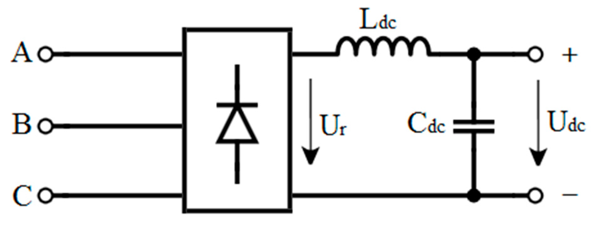
The three-phase rectifier from
Figure 3 was simulated using the concept of commutation functions [
22].
In this case, the state of each diode of the rectifier is represented by the following general equation:
Using this representation, the rectified current and voltage can be written according to the following formulas:
where α and β are components of both the phase currents and the switching functions, and are calculated using the CLARKE matrix transformation:
where
is the DC current smoothing inductance,
is the inductance equivalent resistance, and
is the DC voltage. In the above equations, the zero component was not used because it was assumed that the generator produces a balanced three-phase voltage system.
The two DC/DC converters were modeled according to the same principle, state space representation. According to the control theory, a dynamic system can be represented in state space form by using the following formulae:
where
is the time derivative of
, called the state vector;
is the output vector;
is the state matrix;
is the input matrix;
is the output matrix; and
is the feedback matrix.
The state variables are the smallest possible subset of system variables that can represent the entire state of the system at any given time; these variables are the ones that appear in the time derivative in the equations of the system.
Considering the basic schematics of both the buck and boost converters, these state variables are the current that flow in the inductance and the voltage that appears across the capacitor. Because they both are switching converters and by considering continuous current conduction (the current through the inductance is always non zero), the actual model is composed of two sub-models that follow the switch state when it is either open or closed.
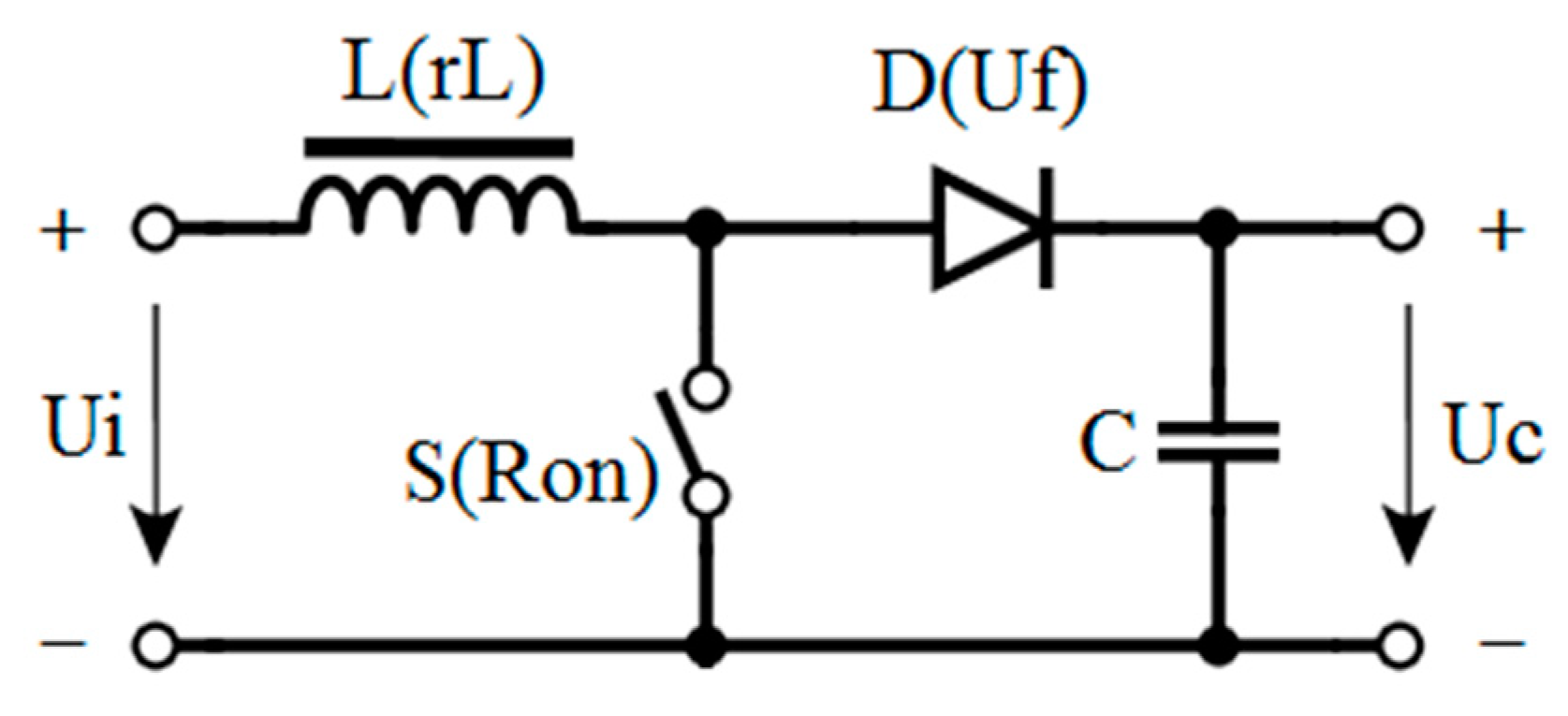
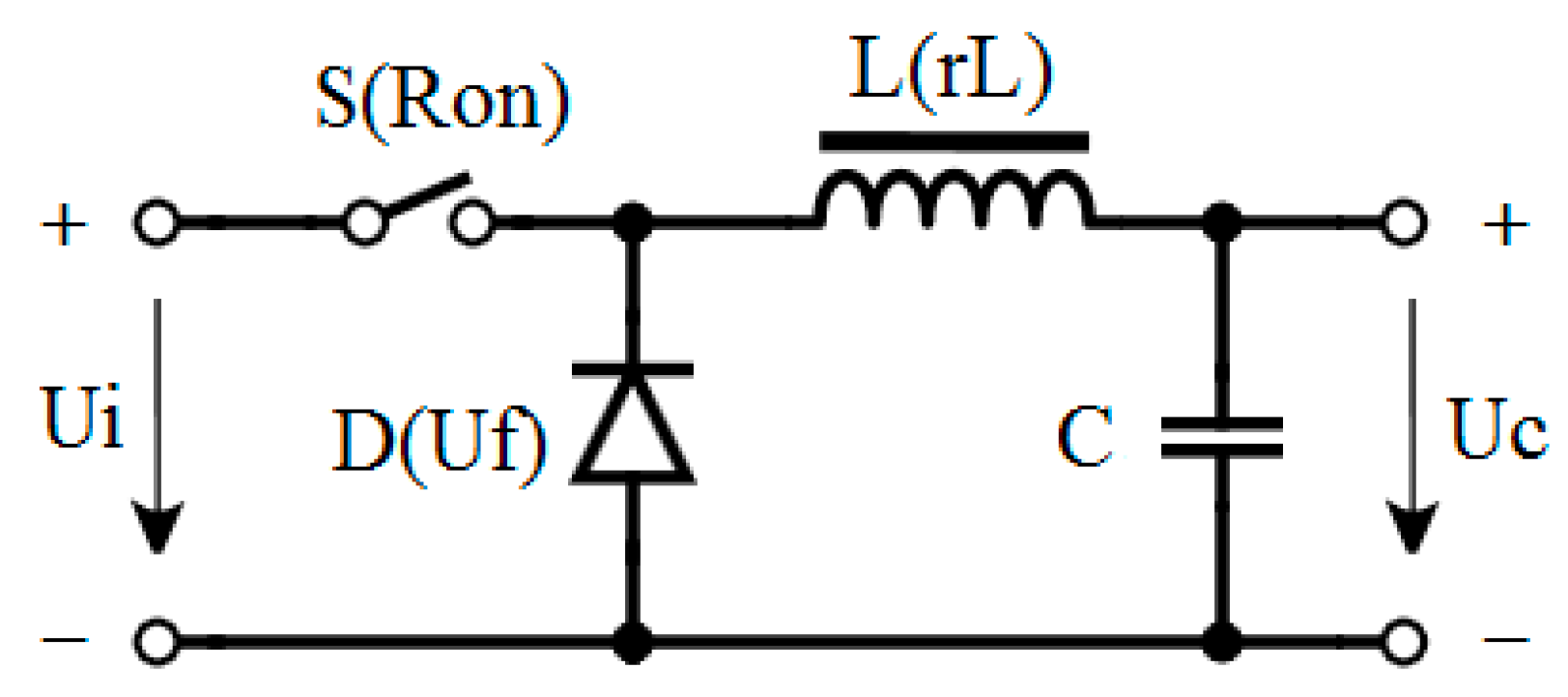
In the following section, the state space models are determined for both boost and buck converter. These models also include part of the parasitic elements that real components have, such as the resistance of the inductance, , the on state resistance of the switch, , and the forward voltage drop of the diode, . They were chosen as a compromise between having a model that is closer to reality and the simulation speed.
The model for the boost converter shown in
Figure 4 has two states: on and off.
Rearranging these equations, we obtained the following state space representation:
The state space representation is:
By using the averaging method over one switching period, we could determine the complete state space model of a boost converter.
where
is the duty cycle, the amount of time the switch is on in one switching cycle. Using Equations (20) and (21), we determined the state matrix and input matrix:
The model for the buck converter is shown in
Figure 5.
The buck converter state space model was designed in a similar way to the boost converter, by writing the equations when the switch was on and off, identifying the state and output matrix, and using state averaging to obtain the full model.
By using the same method, we obtained the following final state and output matrix:
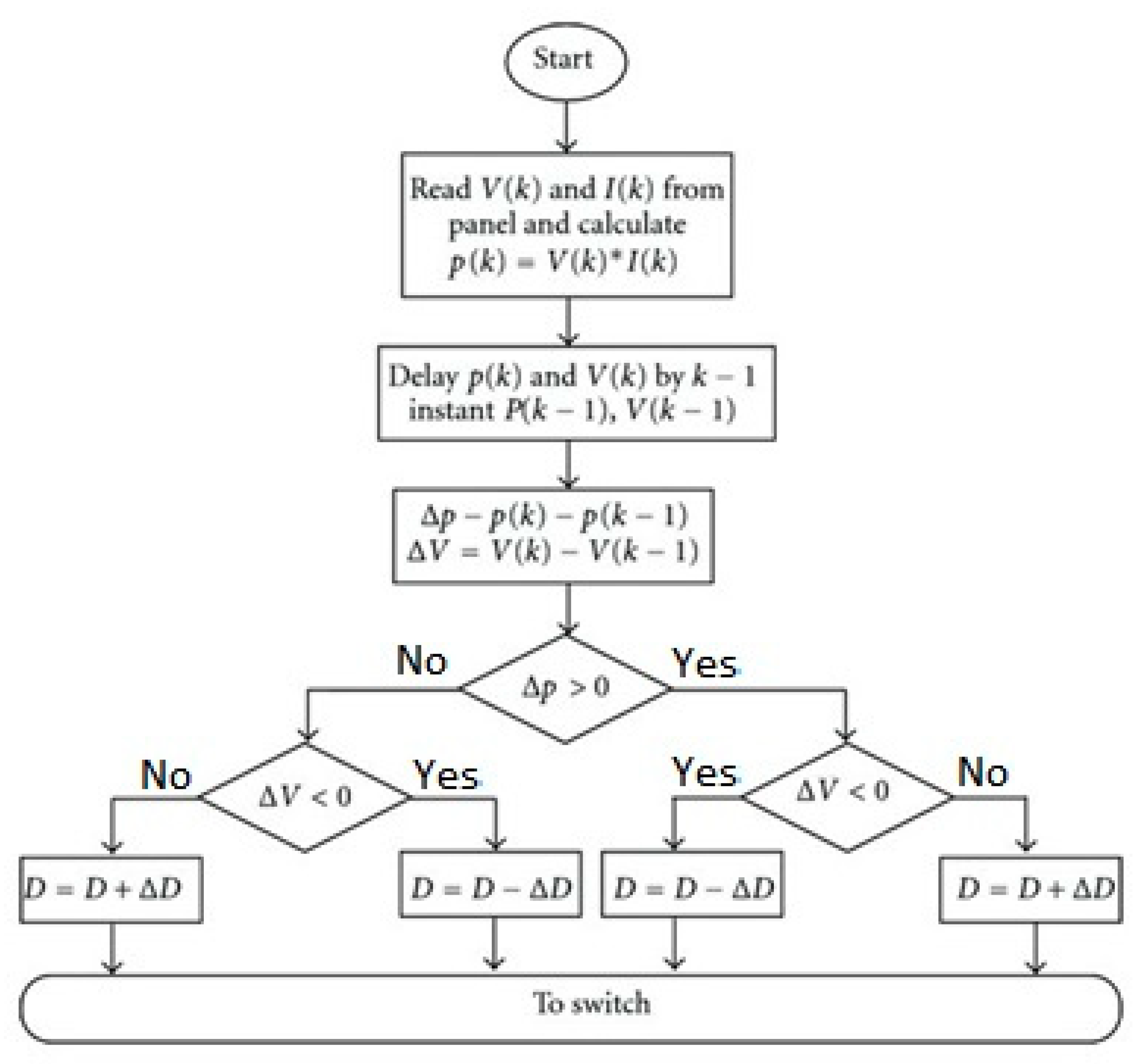
The final step to complete the simulation model, and the most important one, is to introduce the MPPT algorithm that controls the boost converter. Because of its simplicity and overall good performance, we implemented a simple perturb and observe (P&O)-type method.
The power versus rotational speed curve of the hydrokinetic turbine (
Figure 1) shows that the power increases up to a certain speed, after which it decreases. Because the output voltage is directly proportional to the rotational speed for a PMSG, by making small changes to the voltage output (“perturb” and then measure, “observe”, the power output), one can determine where the operating point is on the curve. The general description of the algorithm is given in the following flowchart representation from
Figure 6.
One drawback of this method is that it requires some tuning of the perturbation increment, which is different for each application. If the perturbation increment is too small, the system requires a longer time to reach the maximum power point; if the increment is too large, the system has significant oscillations around the maximum power point.
Other methods are available [
24,
25,
26], such as the incremental conductance method, where instead of measuring the power, conductance (current over voltage) is measured along the power curve. This has the advantage of no oscillations at the maximum power point but it requires a more sophisticated algorithm implementation. Finally, the buck converter is controlled according to the application requirements. For the considered case, the load being resistive, the duty cycle of the converter can be directly imposed. The specific parameters for different components are presented in
Table 1. For the simulated MPPT algorithm, the parameters of the electric generator of the hydrokinetic turbine previously tested in real operating conditions were implemented. Moreover, the parameters of the same turbine rotor were considered. The initial values of the boost and buck converters were calculated by using standard equations; because of the instabilities of the control algorithm, these parameters along with a suitable load were adjusted until the desired response was obtained.
3. Findings and Interpretation of Results
The algorithm used the specific parameters of the previously tested turbine system (rotor and electric generator) [
21], as shown in
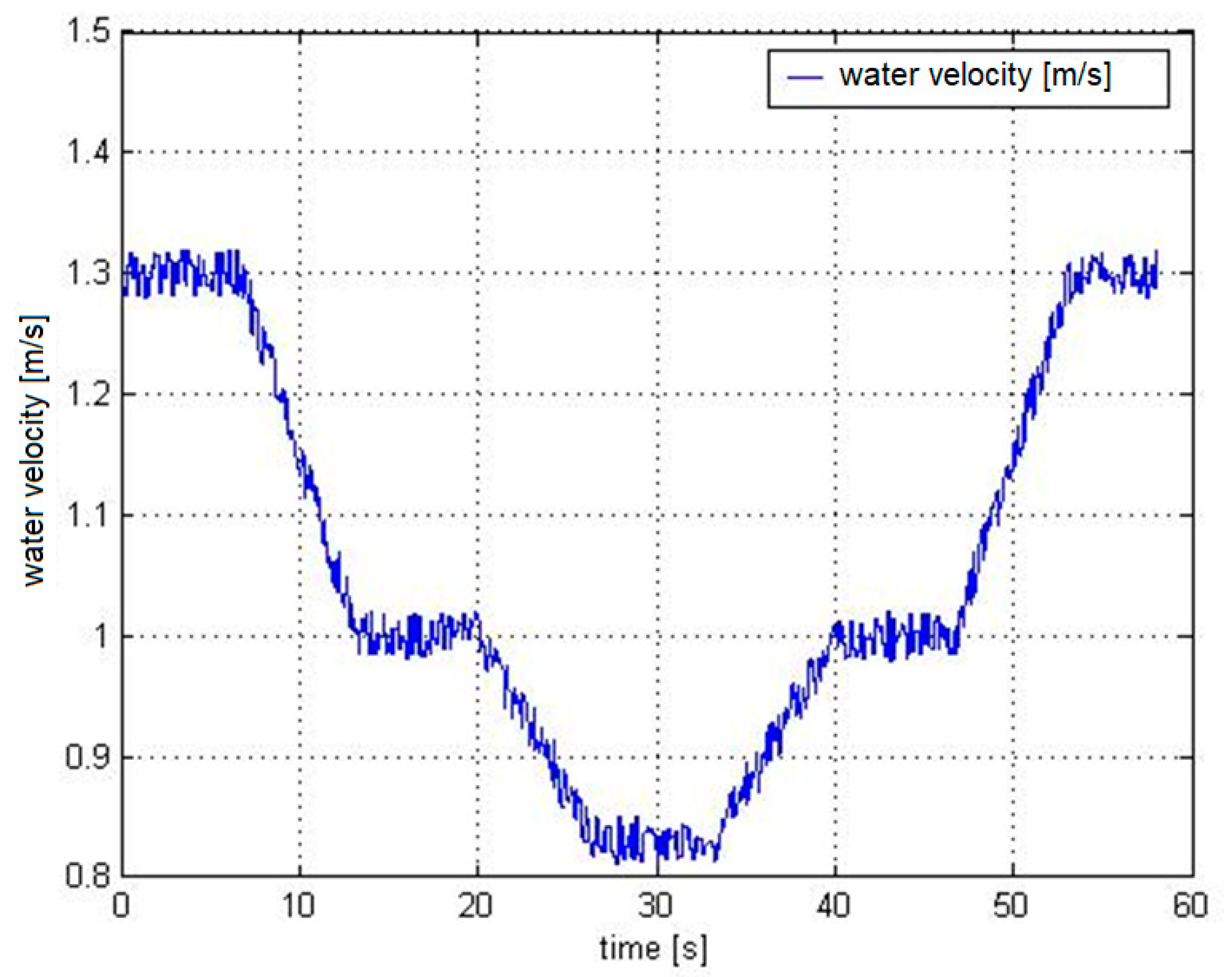
Table 1. The simulation was performed for the same water velocities for which the turbine had been tested. Thus, the variation of the water velocity decreasing from 1.33 m/s to 1 m/s and further to 0.83 m/s was considered. This enabled the validation of the simulation with the experiments that had been carried out in [
21]. The simulated water velocity variation over time is shown in
Figure 7. Various water velocity profiles were considered in order to represent, as realistically as possible, the water flow by adding white noise and a gradual transition from one velocity value to another.
The correction Δ
D applied increases or decreases the duty cycle of the converter.
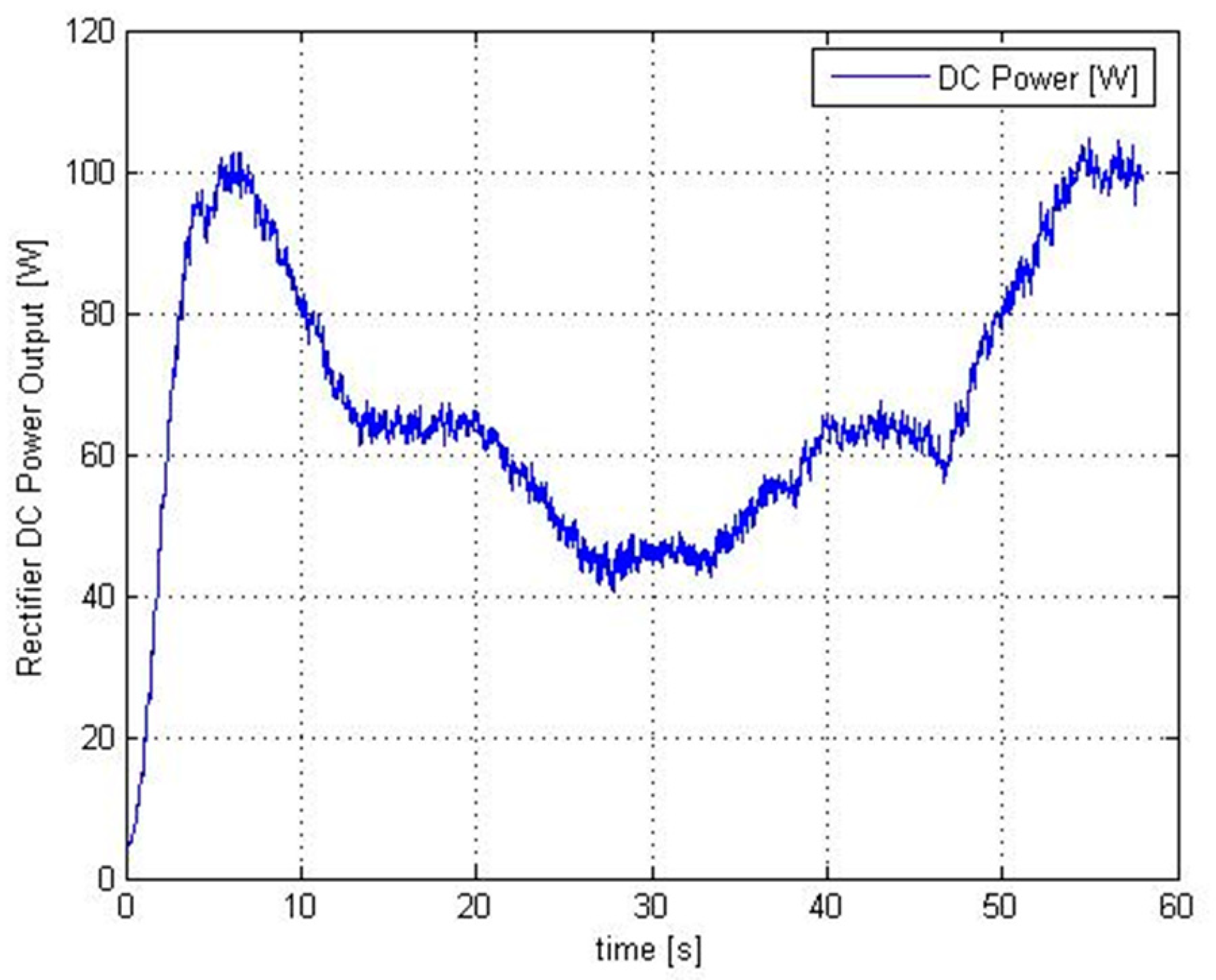
Figure 8 shows the variation of rectified DC power in response to the MPPT correction as the water velocity changed. It can be seen that the power output closely followed the variation of the water velocity, which, in turn, determined the change of the rotational speed of the generator.
Analyzing the graphs shown in
Figure 1 and
Figure 8, we can compare the results of the performed simulation to the experimental results obtained during on-site testing. The results are summarized in
Table 2.
According to
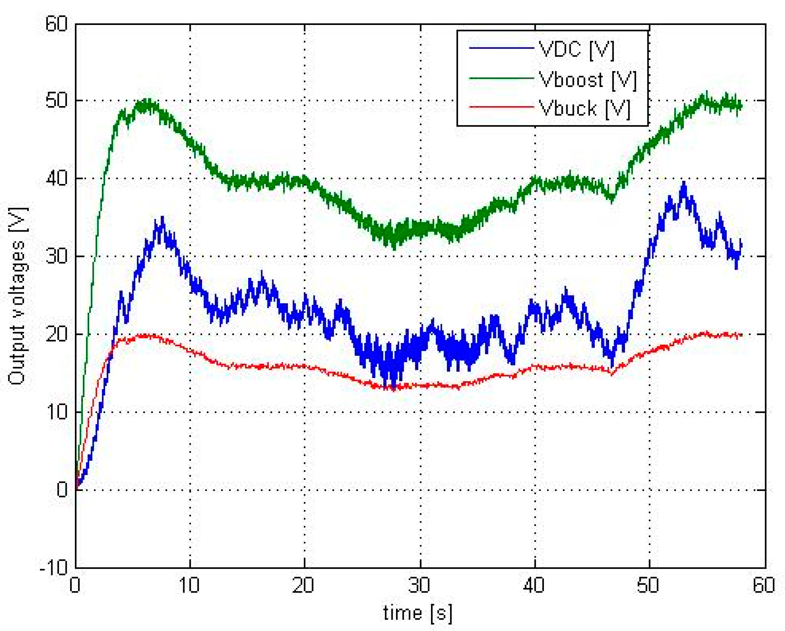
Table 2, the simulation predicted a power output of 105 W for a water velocity of 1.33 m/s, 60 W for 1 m/s, and 30 W for 0.83 m/s. The algorithm provided more accurate results for increased water velocities (≥1 m/s) because at lower velocities the low voltage output determines system instabilities when trying to ensure a stable voltage output, as seen in
Figure 9 (Vdc). This occurs due to the fact that the system has an increased voltage threshold that is necessary to ensure the specification of the load, especially if considering a battery charging system.
Because the first DC converter was a boost-type converter, the correction (which was actually the duty cycle of the converter) decreased. Therefore, the output voltage of the converter increased, as shown in
Figure 9, along with the increase in the rectifier DC power from
Figure 8, as the algorithm tracked the maximum point for the particular water velocity. It was found that the response time to a change in velocity was fast. However, once the maximum point was reached, there were small oscillations in MPPT correction, as expected for this type of algorithm; these oscillations can be reduced by a more precise tuning of the MPPT increment factor and the sampling time of the algorithm.
Figure 9 shows all the three voltages: the rectifier output voltage (blue); the DC boost converter output voltage (green); and the buck converter output voltage, Vbuck (red). The buck converter output fed a resistive load that was simulated considering the duty cycle was set to 40%, as can be seen in the block diagram from
Figure 2.
As shown in
Figure 9, the buck converter maintained the voltage in a narrow range and operated as expected; thus, it was demonstrated that its role is essential in stabilizing the Vdc voltage, which has significant variations after the boost converter.
The limitations of the algorithm are related to using a pure resistive load instead of a battery model, which would better simulate a realistic system. If the considered load cannot use the whole power provided by the turbine, then there may be losses in the operation of the system. This can be overcome by using a battery system to store the power which is not needed at a certain time. Therefore, future research directions may focus on improving the algorithm by considering a battery between the buck converter and load. The simulated algorithm can be integrated in a hardware device provided with storage (battery + BMS), which will maximize the extracted power. This kind of device can be suitable for all types of low-power applications (phone charging, night lighting, signaling, data communication, etc.).

 ,
, 


