Evolution of a Geothermal System with Fluid Re-Injection

Abstract

In this paper, we study the stationary configurations of a vapor-dominated geothermal system. We propose a general mathematical model, which turns out to be a free boundary problem, and we focus on the stationary solutions. The analysis, developed considering the data of the geothermal field in Larderello, Tuscany (Italy), shows that steady-stable states may exist both when the re-injection takes place in depth and when the natural recharge is distributed both in the area occupied by vapor and in the one occupied by liquid.

1. Introduction

In volcanic areas, geothermal energy represents an important resource. For instance, the Tuscan basins of Larderello and Monte Amiata provide almost 30% of the energetic need of the whole region (see, for example, [1,2]). Several studies have been devoted to geothermal reservoirs with the aim of providing mathematical models—some of them very sophisticated—for extraction wells [3,4,5,6,7,8,9,10]. Here we refer to a specific situation—a vapor-dominated system [11,12]—in which the reservoir is sealed at the top by a nearly impermeable rock layer, under which water is in the vapor state up to a depth at which the pressure and temperature are such that it is present as liquid. Wells are drilled through the impermeable layer to reach the high-pressure vapor zone. The vapor then leaves the reservoir, and extraction is sustained by the vaporization of deep water (sometimes called plutonic or juvenile water). This is the case for the Larderello geothermal system (one of the largest in the world), which is characterized by a reservoir pressure that is much lower than hydrostatic pressure. This is a consequence of its natural evolution from an initial liquid-dominated to the current vapor-dominated system [3,10].

The genesis of vapor-dominated reservoirs has intrigued researchers for many years. In 1973, Truesdell and White [6] reviewed all the principal conceptual models proposed until then for the reservoir and possible mechanisms for superheating the steam. These models aimed to give a qualitative description of the physical processes leading to the development of a vapor-dominated reservoir. However, all efforts notwithstanding, many open questions remain.

A reservoir is always formed by a complex of fractured permeable rocks confined between impermeable layers and saturated by water, in a liquid and/or vapor phase. As far as the Larderello geothermal field is concerned, the heat source is a magmatic intrusion located at a relatively small depth (5–10 km) producing temperatures of 500 $÷$ 700 °C in the rocks surrounding the reservoir. Both the lower and upper boundaries of the reservoir depend on the local lithology. The so-called K horizon (a seismic reflecting surface), strictly related to a temperature of about 450 ${}^{\circ }\mathrm{C}$, is considered to represent the bottom of the geothermal reservoir [10,13,14]. The top of the productive reservoir is set in correspondence to the first fractured level in the central areas of the field, where a great amount of well data are available. In the peripheral areas, where well data are lacking, the top is set in correspondence to the 250 ${}^{\circ }\mathrm{C}$ isotherm [13,14,15,16]. Usually, the shallow carbonate–anhydrite reservoir shows a temperature of $220÷250$ ${}^{\circ }\mathrm{C}$ and pressure of about $15÷20$ bar at 1000 m depth, while the deep metamorphic reservoir has a temperature of $300÷350$ ${}^{\circ }\mathrm{C}$ and pressure around 70 bar at 3000 m depth [13].

The sustainable management of geothermal resources basically involves setting up and maintaining a specific long-term production scheme [17,18]. It also involves the basic ingredients of successful geothermal resource management; i.e., re-injection, monitoring and modeling [14,19,20]. However, the term “sustainable development” has many other important implications and has received ever-increasing attention over the last decade or two [21,22,23,24,25,26,27,28,29].

Vapor-dominated geothermal fields are still little understood, and their production histories are so short that premonitory indications of exhaustion are not yet generally recognized. In the 1970s, Sestini [30] concluded that the production of steam from the Larderello fields at that time was approaching a steady state and could have been maintained for many years. However, Truesdell and White [6] came to quite different conclusions, saying that the Larderello field was approaching exhaustion. This appears to have been sustained 30 years later, as the time series of production shows, in the papers by Romagnoli et al. [10] and Barelli [9]. In this context, the study of water levels reported in 1978 by Celati et al. [31] is of great importance.

In the last 20 years, due to the increase of the power demand from renewable sources, many studies have investigated the Larderello–Travale geothermal field using fully three-dimensional models [10,14,32,33,34]. Clearly, the reliability of the forthcoming conclusions of these approaches depends heavily upon the reliability of the boundary and initial conditions selected. In general, these studies are validated against the current rates of production with the aim of predicting future scenarios.

The present contribution focuses on the modeling of geothermal systems in which extraction, natural and artificial recharge mechanisms may act simultaneously. Indeed, the extracted geothermal fluid, after its utilization in a power plant, can be injected back into the reservoir through specific injection wells. For instance, in Larderello, re-injection activities started in the 1970s to contrast the production decline [2,13]. In this way, the natural recharge of the reservoir (by meteoric or juvenile water) is artificially integrated, drastically reducing the impact on the environment of power-plant operations [35,36].

The aim of this study is to investigate the existence and stability of possible equilibrium configurations that can guarantee sustainable production. We develop a model that is able to give some basic information. Of course, approximations have been introduced in order to develop a model which is mathematically treatable. For example, the fluid in the reservoir is assumed to be pure water; this is a very schematic description, as, in practice, many chemicals are carried by the water, which makes the real thermodynamics much more complex. Next, we consider a region with a cluster of wells distributed so that the vapor motion underneath can be reasonably considered to be one-dimensional. This may appear to be an excessive approximation, but actually it is largely justified by the fact that problems such as this are characterized by a great level of data uncertainty. Our model is a one-dimensional parabolic free boundary problem, where both extraction and recharge are treated as source terms in the continuity equation. In this framework, we develop a model describing the behavior of the geothermal field, the location of the water vaporization front and its stability with respect to perturbations. More precisely, we examine the steady (or quasi-steady) state attained by recharging the reservoir with water, looking for those recharging rates compatible with a stable state. In particular, we discuss the effects of both extraction and recharge (both natural and artificial). We determine the steady solution by solving a non-linear equation which, when peculiar conditions are met, has more than a single solution. A linear stability analysis of the stationary liquid/vapor interface (if it exists) is then used to select the physically acceptable solution. In particular, we show that selecting the parameters according to the field data allows us to obtain a stable interface that is qualitatively in agreement with the borehole extraction/injection data. In this respect, our model, although extremely simple, allows us to obtain some insights regarding the state of the reservoir and to predict the location of the phase transition surface. On one hand, the simplicity of the model has the advantage that one can deal with an exact solution; on the other hand, the price to pay is that a classical validation remains questionable, as a sharp liquid/vapor interface is very unlike to exist in a real field. However, it should also be taken into account that that even highly sophisticated three-dimensional models depend significantly upon the boundary and initial conditions imposed. In the majority of cases (and for Larderello in particular), these conditions suffer from a great degree of uncertainty that greatly influences the reliability of the model predictions.

The paper continues as follows. Section 2 is devoted to the general 1D model. The analysis of the stationary solutions is illustrated in Section 3 and Section 4. In Section 5, we relate the results to some historical field data for a better interpretation and justification of the model. The conclusions are drawn in the last section.

2. The Mathematical Model

We consider a geothermal fluid composed of water in a gaseous and liquid state. We denote by x the vertical axis pointing upward. The bottom and the top of the geothermal reservoir correspond to $x=L_i$$(L_i<0)$ and to $x=L_s$$(L_s<0)$, respectively. The ground surface corresponds to $x=0$, so that the domain of interest is $\left[L_i,L_s\right]$. We assume that the width of the capillary fringe is negligible with respect to the vertical dimensions of the reservoir, and thus that there is a clear separation between the liquid and the vapor phase through a sharp interface, $x=s\left(t\right)$, that may vary in time. So, the lower part of the domain $L_i\le x\le s\left(t\right)$, is saturated with liquid, while in the upper part of the domain, $s\left(t\right)\le x\le L_s$, there is only vapor. At $x=L_s$ the vapor pressure is known, and we denote it as $P_s$. The latter is a measured datum and essentially depends on the exploitation of the basin.

In

Table 1. List of parameters referring to the reservoir of Larderello [10,14]. All dimensionless constants used in the present work are evaluated by using these values. A full list of additional simbols is reported in Table 3.

Symbol	Description	Value	Units
$L_s$	Reservoir top depth	$-1000$	$\mathrm{m}$
$L_i$	Reservoir bottom depth	$-3500$	$\mathrm{m}$
$T_s$	Temperature at the top of the reservoir	550	$\mathrm{K}$
$\gamma$	Thermal gradient	$0.04$	$\mathrm{K}/\mathrm{m}$
$P_s$	Vapor pressure at the top of the reservoir	$9\times {10}^5$	$\mathrm{Pa}$
r	Universal gas constant over H${}_2$O molar mass	$4.6\times {10}^2$	$\mathrm{J}/\left(\mathrm{k}\mathrm{g}\mathrm{K}\right)$
${\rho }_l$	Liquid water density (at local conditions)	≈$8\times {10}^2$	$\mathrm{k}\mathrm{g}/{\mathrm{m}}^3$
$\varphi$	Medium porosity	$2\times {10}^{-2}$	-
g	Standard gravity	$9.8$	$\mathrm{m}/{\mathrm{s}}^2$
$\mu$	Vapor viscosity	$2\times {10}^{-5}$	$\mathrm{Pa}\mathrm{s}$
$\kappa$	Medium permeability	≈$5\times {10}^{-15}$	${\mathrm{m}}^2$
$K_T$	Thermal conductivity	≈2	$\mathrm{W}/\left(\mathrm{m}K\right)$

, we list the values of the constants involved in the model. These parameters are compatible with those available for some areas of the geothermal field of Larderello, Tuscany [10,14].

According to the experimental data [37,38,39], the temperature within the reservoir is linear:

$$T\left(x\right)=T_s+\gamma \left(L_s-x\right),L_i\le x\le L_s,$$

(1)

where $\gamma >0$, constant in time, is the known thermal gradient (see Table 1). We also set

$$L=L_s-L_i(=2500\mathrm{m}).$$

(2)

Remark 1.

The given value of γ in Table 1 implies that the temperature at depth $L_i=-3500\mathrm{m}$ is $650\mathrm{K}$. Assuming a surface temperature of $300\mathrm{K}$, we have a geothermal gradient in the caprock of ${\gamma }_{\mathrm{cap}}=0.25\mathrm{K}/\mathrm{m}$. This may be surprising, since this value is about three times the value commonly indicated in textbooks as the typical gradient in a geothermal field (generally $0.08\mathrm{K}/\mathrm{m})$ and actually requires that the average thermal conductivity of the caprock be rather low—say $0.32\mathrm{W}/\left(\mathrm{m}\mathrm{K}\right)$. A simple explanation is that the mean gradient of the field is indeed based upon the estimated depth of the K horizon (in the present case, around $-5000\mathrm{m}$) and the isotherm which identifies the K horizon itself (about $750\mathrm{K}$), leading, correctly, to ${\gamma }_{\mathrm{mean}}=0.08\mathrm{K}/\mathrm{m}$. On the other hand, the question is much more complex. In a very recently published article [39], the great variability of the thermal conductivity $K_T$ of rocks at Larderello and their strong dependence on temperature and, to a much lesser extent, on pressure were clearly emphasized. Reported values vary from less that $2\mathrm{W}/\left(\mathrm{m}\mathrm{K}\right)$ to more then $4.5\mathrm{W}/\left(\mathrm{m}\mathrm{K}\right)$ depending on the core sample depth and exploration well. Furthermore, the evaluated geothermal gradient has a great variability with depth, reaching values, for some layers, close to ${\gamma }_{\mathrm{cap}}=0.2\mathrm{K}/\mathrm{m}$—not far from the value proposed in Table 1.

The domain $s\left(t\right)\le x\le L_s$ is saturated by vapor whose continuity equation is

$$\frac{\partial }{\partial t} \left(\varphi \rho \right) +\frac{\partial }{\partial x} \left(\varphi \rho v\right) =\varphi d_v,s\left(t\right)<x\le L_s,$$

(3)

where $\varphi \left(x\right)$ is medium porosity (see Table 1), v is the velocity of the vapor, $\rho$ is its density and $d_v$ is the vapor source/sink density rate (with dimensions $\mathrm{k}\mathrm{g}{\mathrm{m}}^{-3}{\mathrm{s}}^{-1}$). In general, $d_v$ is due to both the recharge vapor (generated from the vaporization of meteoric recharge water), which mixes with the vapor inside the reservoir, and the extraction/re-injection due to external devices [40]. In general, the rate $d_v$ depends on the local pressure, or rather on the difference between the external pressure and the local pressure. More specifically, we split $d_v$ into two contributions: a recharge generated from the vaporization of recharge water (which may depend on the local pressure) and a point-wise recharge due to N injection/extraction wells whose extraction/injection rates depend on the difference between the local pressure and the re-injection pressure:

$${\displaystyle d_v=d_{v,\mathrm{met}}\left(P\right) + \sum _{i=1}^N{d}_{v,\mathrm{inj}}^{\left(i\right)}{J}_v^{\left(i\right)} \left(P-P_{\mathrm{inj}}^{\left(i\right)}\right) \delta \left(x-x_i\right) ,}$$

(4)

where the subscripts “met” and “inj” mean, respectively, “of meteoric origin” and “due to injection”, P denotes the vapor pressure, $\delta$ denotes the Dirac delta, $x_i$ is the location of the ith injection head, $d_{v,\mathrm{inj}}^{\left(i\right)}$ is the order of magnitude of the density rate, where $J_v^{\left(i\right)}$ (dimensionless) gives its dependence on the pressure difference, and $P_{\mathrm{inj}}^{\left(i\right)}$ is the injection pressure.

The vapor is assumed to behave as a perfect gas; i.e.,

$$\rho =\frac{P}{rT},$$

(5)

where r is the molar vapor constant (see Table 1). Using the generalized Darcy’s law [41],

$$\varphi v=-\frac{\kappa }{\mu \left(P,T\right)}\left(\frac{\partial P}{\partial x}+\rho g\right),$$

(6)

where $\mu$ is the vapor viscosity, which depends on both temperature and pressure, and $\kappa \left(x\right)$ is the permeability of the medium (see again Table 1), $\rho$ is as in Equation (5) and g is the gravity acceleration; thus, we rewrite (3) as

$$\frac{1}{T}\frac{\partial P}{\partial t}-\frac{1}{\varphi \left(x\right)}\frac{\partial }{\partial x}\left[\frac{\kappa \left(x\right)P}{\mu \left(P,T\right)T}\left(\frac{\partial P}{\partial x}+\frac{g}{r}\frac{P}{T}\right)\right]=r{d}_v\left(P\right),s\left(t\right)<x\le L_s<0,$$

(7)

where T is given by (1).

In the liquid region $L_i\le x\le s\left(t\right)$, the continuity equation is written as

$$\frac{\partial \varphi {\rho }_{\ell }}{\partial t}+\frac{\partial }{\partial x}\left(\varphi {\rho }_{\ell }{v}_{\ell }\right)={\rho }_{\ell }\varphi d_{\ell },L_i\le x\le s\left(t\right),$$

(8)

where ${\rho }_{\ell }$ is the density of the liquid, $v_{\ell }$ is the liquid velocity and $d_{\ell }$ is the liquid water source density rate (with a dimension of ${\mathrm{s}}^{-1}$), due to both re-injection and natural recharge fluid. The solution to Equation (8) is

$$v_{\ell }(x,t)=\frac{1}{\varphi \left(x\right){\rho }_{\ell }\left(T,P\right)}{\int }_{L_i}^x\varphi \left(\xi \right)\left(d_{\ell }{\rho }_{\ell }-\frac{\partial {\rho }_{\ell }}{\partial t}\right)d\xi ,L_i<x<s\left(t\right)\le L_s<0,$$

(9)

where, for simplicity, we have neglected $v_{\ell }\left(L_i,t\right)$, and where the pressure P is the hydrostatic pressure.

The continuity of the mass flux across $s\left(t\right)$ implies that $\rho v-{\rho }_{\ell }{v}_{\ell }=-\dot{s}\left({\rho }_{\ell }-\rho \right)$ [42]. As $\rho \ll {\rho }_{\ell }$, we can approximate this relation with

$$\dot{s}=\left(1+\frac{\rho }{{\rho }_{\ell }}\right)v_{\ell }-\frac{\rho }{{\rho }_{\ell }}v.$$

(10)

Thus, recalling Equations (6) and (9), we obtain

$$\dot{s}=D_{\ell }{\left(1+\frac{P}{{\rho }_{\ell }rT}\right)}_{x=s\left(t\right)}+{\left[\frac{P}{rT{\rho }_{\ell }}\frac{\kappa }{\varphi \mu }\left(\frac{\partial P}{\partial x}+\frac{P}{rT}g\right)\right]}_{x=s\left(t\right)},$$

(11)

where

$$D_{\ell }=\frac{1}{{\left(\varphi {\rho }_{\ell }\right)}_{x=s\left(t\right)}}{\int }_{L_i}^{s\left(t\right)}\varphi \left(\xi \right)\left(d_{\ell }{\rho }_{\ell }-\frac{\partial {\rho }_{\ell }}{\partial t}\right)d\xi ,$$

(12)

which (with a dimension of $\mathrm{m}{\mathrm{s}}^{-1}$) is the total recharge rate in the liquid domain. In particular, we assume that we can identify two distinct effects:

(i)

Recharge due to the meteoric waters, denoted by $d_{\ell ,\mathrm{met}}$, which, as $d_{v,\mathrm{met}}$, may depend on the local pressure;

(ii)

Recharge due to clusters of re-injection wells which, for simplicity, we assume to be concentrated in M locations.

Thus, setting

$$d_{\ell }\left(x\right)=\underset{\mathrm{recharge}}{\underset{\mathrm{meteoric}}{\underbrace{d_{\ell ,\mathrm{met}}}}}+\underset{\mathrm{re}-\mathrm{injection}}{\underbrace{{\displaystyle \sum _{i=i}^M{d}_{\ell ,\mathrm{inj}}^{\left(i\right)}{J}_{\ell }^{\left(i\right)}\left(P\left(x_i\right)-P_{\mathrm{inj}}^{\left(i\right)}\right)\delta \left(x-x_i\right)}}},$$

(13)

where, as in (4), the injection rates depend on the difference between the re-injection pressure $P_{\mathrm{inj}}$ and the local pressure. Indeed, $d_{\ell ,\mathrm{inj}}^{\left(i\right)}$, $i=1,2,$$\dots$, M, gives the injection rate order of magnitude, while $J_{\ell }^{\left(i\right)}\left(P\left(x_i\right)-P_{\mathrm{inj}}^{\left(i\right)}\right)$, which is dimensionless, gives the dependence on the pressure difference. We thus have

$$\begin{array}{ccc}\hfill D_{\ell }& =& {\displaystyle \frac{{\displaystyle {\int }_{L_i}^{s\left(t\right)}\varphi \left(\xi \right)\left[\left({\displaystyle d_{\ell ,\mathrm{met}}+\sum _{i=i}^M{d}_{\ell ,\mathrm{inj}}^{\left(i\right)}{\mathcal{L}}_{\ell }^{\left(i\right)}\left(\xi \right)}\right){\rho }_{\ell }-\frac{\partial {\rho }_{\ell }}{\partial t}\right]d\xi }}{\varphi \left(s\left(t\right)\right){\left.{\rho }_{\ell }\left(T,P\right)\right|}_{s\left(t\right)}}}\hfill \\ & =& {\displaystyle \frac{{\displaystyle d_{\ell ,\mathrm{met}}{\int }_{L_i}^{s\left(t\right)}\varphi \left(\xi \right)\left[\left({\displaystyle 1+\sum _{i=i}^M\frac{d_{\ell ,\mathrm{inj}}^{\left(i\right)}}{d_{\ell ,\mathrm{met}}}{\mathcal{L}}_{\ell }^{\left(i\right)}\left(\xi \right)}\right){\rho }_{\ell }\left(P,T\right)-\frac{\partial {\rho }_{\ell }\left(P,T\right)}{\partial t}\right]d\xi }}{\varphi \left(s\left(t\right)\right){\left.{\rho }_{\ell }\left(T,P\right)\right|}_{s\left(t\right)}}}.\hfill \end{array}$$

where

$${\mathcal{L}}_{\ell }^{\left(i\right)}\left(x\right)=J_{\ell }^{\left(i\right)}\left(P\left(x\right)-P_{\mathrm{inj}}^{\left(i\right)}\right)\delta \left(x-x_i\right)$$

(14)

A second free boundary condition is provided by Clapeyron’s law, which gives the relationship between P and T at the liquid/vapor interface. In the range of temperature relevant to our problem, this law takes the following empirical form:

$$P^{*}=aexp\left[b\frac{T-273}{T}\right],$$

(15)

where T is in Kelvin, P in Pascal and a and b have values of $a=9.617\times {10}^2\mathrm{Pa}$, $b=17.35$. Consequently, the second condition on the free boundary is

$$P\left(s\left(t\right),t\right)=P^{*}\left(T\left(s\left(t\right)\right)\right),$$

(16)

and (11) rewrites as

$$\begin{array}{ccc}\dot{s}\hfill & =\hfill & D_{\ell }{\left[1+{\displaystyle \frac{P^{*}}{rT{\rho }_{\ell }}}\right]}_{x=s\left(t\right)}\hfill \\ \hfill & \hfill & \\ \hfill & +\hfill & {\left[{\displaystyle \frac{P^{*}}{rT{\rho }_{\ell }}}{\displaystyle \frac{\kappa }{\varphi \mu }}\left({\displaystyle \frac{\partial P}{\partial x}}+{\displaystyle \frac{P^{*}}{rT}}g\right)\right]}_{x=s\left(t\right)}.\hfill \end{array}$$

(17)

We remark that (16) requires the following condition be fulfilled:

$$P\left(x,t\right)<P^{*}\left(T\left(x\right)\right),\mathrm{in}\mathrm{the}\mathrm{vapor}\mathrm{domain};\mathrm{i}.\mathrm{e}.,s\left(t\right)<x\le L_s,$$

(18)

in order to obtain a physically consistent solution.

To complete the information, we need to give the pressure at the reservoir top, $P\left(L_s,t\right)=P_s$ (see Table 1) and the initial conditions $s\left(0\right)=s_o$, $L_i<s_o<L_s$, $P\left(x,0\right)=P_o\left(x\right)$, $s_o<x<L_s$, fulfilling Equations (18) and (16); i.e., $P_o\left(x\right)<P^{*}\left(T\left(x\right)\right)$ and $P_o\left(s_o\right)=P^{*}\left(T\left(s_o\right)\right)$.

Thus, the mathematical problem to be solved is the following: find a time $\tau >0$, a function $s\left(t\right)\in C\left[0,\tau \right]\cap C^1\left(0,\tau \right)$ such that $s\left(t\right)\in \left(L_i,L_s\right)$ and a function $P\left(x,t\right)\in C^{2,1}\left(D_{\tau }\right)$, continuous in ${\overline{D}}_{\tau }=\left\{\left(x,t\right)\mid s\left(t\right)\le x\le L_s,0\le t\le \tau \right\}$, where ${\partial }_{x}P$ is continuous up to $x=s\left(t\right)$, $t\in \left(0,\tau \right)$, so that, for $T\left(x\right)$ given by Equation (1), the following system is fulfilled:

$$\left\{\begin{array}{cccc}{\displaystyle \frac{\partial P}{\partial t}}-{\displaystyle \frac{T}{\varphi }}{\displaystyle \frac{\partial }{\partial x}}\left[{\displaystyle \frac{\kappa P}{T\mu }}\left({\displaystyle \frac{\partial P}{\partial x}}+{\displaystyle \frac{g}{r}}{\displaystyle \frac{P}{T}}\right)\right]=rT{d}_v\left(P\right),\left(x,t\right)\in D_{\tau },\hfill & \hfill & & \\ \hfill & \hfill & & \\ P(L_s,t)=P_s,t\in \left[0,\tau \right],\hfill & \hfill & & \\ \hfill & \hfill & & \\ P(s\left(t\right),t)=P^{*}\left(T\left(s\left(t\right)\right)\right),t\in \left[0,\tau \right],\hfill & \hfill & & \\ \hfill & \hfill & & \\ \dot{s}=D_{\ell }{\left[1+{\displaystyle \frac{P^{*}}{rT{\rho }_{\ell }}}\right]}_{x=s\left(t\right)}\hfill & \hfill & & \\ +{\left[{\displaystyle \frac{P^{*}}{rT{\rho }_{\ell }}}{\displaystyle \frac{\kappa }{\varphi \mu }}\left({\displaystyle \frac{\partial P}{\partial x}}+{\displaystyle \frac{P^{*}}{rT}}g\right)\right]}_{x=s\left(t\right)},t\in \left(0,\tau \right),\hfill & \hfill & & \\ \hfill & \hfill & & \\ P(x,0)=P_o\left(x\right),x\in \left[s_o,L_s\right],\hfill & \hfill & & \\ \hfill & \hfill & & \\ s\left(0\right)=s_o,s_o\in \left(L_i,L_s\right),\hfill & \hfill & \end{array}\right.$$

(19)

According to the results in [43,44], the problem has one unique solution provided that $P_o\in C\left[s_o,L_s\right]$.

3. Steady-State Solutions

We consider a steady state (meaning that neither $d_v$ nor $d_{\ell }$ depend on time) and normalize space, temperature and pressure in the following way:

$$\tilde{x}=\frac{x-L_s}{L},\iff \tilde{x}\in \left[-1,0\right],\tilde{s}=\frac{s-L_s}{L},\iff \tilde{s}\in \left[-1,0\right],$$

(20)

$$\tilde{T}=\frac{T}{T_s},\tilde{P}=\frac{P}{P_c},$$

where $P_c$ is a characteristic pressure, which still needs to be selected. Recalling Equation (1), we consider $\tilde{T}$ to be an independent variable; namely

$$\tilde{T}=1-\tilde{\mathrm{\Gamma }}\tilde{x},⟺\tilde{T}\in \left(1,1+\tilde{\mathrm{\Gamma }}\right),$$

(21)

where

$$\tilde{\mathrm{\Gamma }}=\frac{\gamma L}{T_s}\approx 0.18.$$

We remark that, because of the change of the variable in Equation (20), $\tilde{T}=1$ corresponds to the top of the basin while $1+\tilde{\mathrm{\Gamma }}$ to the bottom.

Next, we introduce

$$\tilde{\sigma }\left(t\right)={\left.\tilde{T}\right|}_{\tilde{x}=\tilde{s}\left(t\right)},$$

(22)

as the temperature at the interface, so that

$$\tilde{\sigma }=1-\tilde{\mathrm{\Gamma }}\tilde{s},⟺\tilde{\sigma }\in \left(1,1+\tilde{\mathrm{\Gamma }}\right).$$

(23)

Then, we set

$$f\left(\tilde{\sigma }\right)={\tilde{P}}^{*}\left(\tilde{\sigma }\right)=\frac{a}{P_c}exp\left[b\frac{\tilde{\sigma }-273/T_s}{\tilde{\sigma }}\right].$$

(24)

We also set ${\rho }_{\ell }\left(\tilde{T}\right)={\rho }_{\ell ,o}{\tilde{\rho }}_{\ell }\left(\tilde{T}\right)$, $\mu \left(\tilde{P},\tilde{T}\right)={\mu }_o\tilde{\mu }\left(\tilde{P},\tilde{T}\right)$, $\kappa \left(\tilde{T}\right)={\kappa }_o\tilde{\kappa }\left(\tilde{T}\right)$, with $\tilde{\mu }$, ${\tilde{\rho }}_{\ell }$ and $\tilde{\kappa }$ being dimensionless; $\varphi \left(\tilde{T}\right)={\varphi }_o\tilde{\varphi }\left(\tilde{T}\right)$, with ${\varphi }_o$ giving the porosity order of magnitude, so that

$$\frac{P^{*}\left(T\left(s\left(t\right)\right)\right)}{rT\left(s\left(t\right)\right){\rho }_{\ell }\left(P^{*},T\left(s\left(t\right)\right)\right)}=\left({\displaystyle \frac{P_c}{r{T}_s{\rho }_{\ell ,o}}}\right)h\left(\tilde{\sigma }\right),\mathrm{with}h\left(\tilde{\sigma }\right)={\displaystyle \frac{f\left(\tilde{\sigma }\right)}{\tilde{\sigma }{\tilde{\rho }}_{\ell }\left(\tilde{\sigma }\right)}},$$

(25)

and

$$D_{\ell }=\frac{d_{\ell ,\mathrm{met}}{T}_s}{\gamma }{\tilde{D}}_{\ell },$$

(26)

with

$${\tilde{D}}_{\ell }=\frac{1}{\varphi \left(\tilde{\sigma }\right){\rho }_{\ell }\left(\tilde{\sigma },f\left(\tilde{\sigma }\right)\right)}{\int }_{\tilde{\sigma }}^{1+\tilde{\mathrm{\Gamma }}}\left[{\displaystyle 1+\sum _{i=i}^M{\mathfrak{R}}_{\ell }^{\left(i\right)}{\mathcal{L}}_{\ell }^{\left(i\right)}\left(\tilde{P}\right)}\right]{\rho }_{\ell }\left(\tilde{P},\tilde{T}\right)\varphi \left(\tilde{T}\right)d\tilde{T},$$

(27)

where ${\mathcal{L}}_{\ell }^{\left(i\right)}$ has been defined in Equation (14) and

$${\mathfrak{R}}_{\ell }^{\left(i\right)}=\frac{d_{\ell ,\mathrm{inj}}^{\left(i\right)}}{d_{\ell ,\mathrm{met}}}.$$

(28)

Setting $P_c=P_s$, the steady dimensionless version of problem (19)$,1$, (19)$,2$, and (19)$,3$ is

$$\left\{\begin{array}{cc}{\displaystyle \frac{1}{\varphi \left(T\right)}}{\displaystyle \frac{\partial }{\partial T}}\left[{\displaystyle \frac{\kappa \left(T\right)}{\mu \left(P,T\right)}}{\displaystyle \frac{P}{T}}\left({\displaystyle \frac{\partial P}{\partial T}}-\eta {\displaystyle \frac{P}{T}}\right)\right]=-{\beta }_v\left(T,P\right),\hfill & 1<T<\sigma ,\hfill \\ \hfill & \\ P\left(1\right)=1,\hfill & \\ \hfill & \\ P\left(\sigma \right)=f\left(\sigma \right),\hfill \end{array}\right.$$

(29)

where $\eta ={\displaystyle \frac{g}{r\gamma }}\approx 0.533$, $f\left(\sigma \right)$ is given by Equation (24) and

$${\beta }_v\left(P,T\right) = \left(\frac{{\varphi }_o}{{\kappa }_o}\frac{r{\mu }_o{T}_s^3}{{\gamma }^2{P}_s^2}{d}_{v,\mathrm{met}}\right)\left[{\displaystyle 1+\sum _{i=1}^N{\mathfrak{R}}_v^{\left(i\right)}{J}_v^{\left(i\right)} \left(P-P_{\mathrm{inj}}^{\left(i\right)}\right) \delta \left(T-T_i\right) }\right],$$

(30)

and

$${\mathfrak{R}}_v^{\left(i\right)}=\frac{d_{v,\mathrm{inj}}^{\left(i\right)}}{d_{v,\mathrm{met}}},i=1,2,\dots ,N.$$

(31)

Here and in the following, we omit the “$\tilde{}$” to keep the notation as clear as possible.

The steady (dimensionless) version of (19)$,4$ is

$$F\left(\sigma \right) = 0,$$

(32)

where

$$\begin{array}{ccc}F\left(\sigma \right)\hfill & = \left({\displaystyle \frac{d_{\ell ,\mathrm{met}}{T}_s}{\gamma }}\right) D_{\ell } \left[1+ \left({\displaystyle \frac{P_s}{r{T}_s{\rho }_{\ell ,o}}}\right) h \left(\sigma \right) \right]\hfill & \\ \hfill & \hfill & \\ \hfill & + \left({\displaystyle \frac{{\kappa }_o{P}_s^2\gamma }{{\varphi }_{o}r{\rho }_{\ell ,o}{\mu }_o{T}_s^2}}\right){\displaystyle \frac{\kappa \left(\sigma \right)h\left(\sigma \right)}{\varphi \left(\sigma \right)\mu \left(f\left(\sigma \right),\sigma \right)}}\mathsf{\Omega }\left(\sigma \right),\hfill \end{array}$$

(33)

with

$$\mathsf{\Omega } \left(\sigma \right) = \eta \frac{f\left(\sigma \right)}{\sigma } - {\left.\frac{\partial P}{\partial T}\right|}_{\sigma }.$$

(34)

In Section 4, we see that the set of steady solutions (Equation (32)) depends upon a set of n suitable parameters ${\zeta }_1,\dots {\zeta }_n$. Thus, Equation (32) writes, more precisely,

$$F(\sigma ;{\zeta }_1,\dots ,{\zeta }_n)=0,$$

(35)

where ${\zeta }_{1}and\dots {\zeta }_n$ are dimensionless. Our approach consists first of verifying that $F=0$ can be made explicit, under some limitations, with respect to a specific parameter—say ${\zeta }_1$—that is

$${\zeta }_1 = \mathfrak{F}(\sigma ,{\zeta }_2,\dots ,{\zeta }_n).$$

(36)

Then, we look for the existence of stable, steady solutions to the system (Equations (29) and (32)) by varying the other parameters. Thus, for a given steady state ${\sigma }_{st}$, the study of its stability to small perturbations is reduced to investigate the following:

$$\frac{\partial F}{\partial \sigma } \left({\sigma }_{st},\mathfrak{F}\left({\sigma }_{st},{\zeta }_2,\dots ,{\zeta }_n\right),{\zeta }_2,\dots ,{\zeta }_n\right).$$

(37)

4. Numerical Simulations

In this section, we analyze some specific cases which represent some of the most significant physical situations. For the sake of simplicity, we take ${\tilde{\rho }}_{\ell }\left(\tilde{T}\right)=\mu \left(\tilde{P},\tilde{T}\right)=\tilde{\kappa }\left(\tilde{T}\right)=\varphi \left(\tilde{T}\right)=1$, so that h, given by Equation (25), simplifies to $h\left(\sigma \right)=f\left(\sigma \right)/\sigma$. Next, we assume that the injection rate is independent of the difference between the injection pressure and local pressure, and therefore $J_{\alpha }\left(P-P_{\mathrm{inj}}^{\left(i\right)}\right)=1$, $\alpha =v,\ell$.

There are many cases, and it is impossible to analyze them all. We therefore focus on these issues:

• Recharge due to both liquid groundwater and to vapor injection in the vapor domain;
• Recharge due to groundwater occurring in the whole domain (liquid and vapor) and to vapor extraction/injection localized in the vapor domain;
• Artificial recharge due to liquid injection localized in the liquid domain.

To see the explicit form of Equation (36), it is more convenient to proceed by subsequent steps.

Suppose, for a moment, that ${\beta }_v=0$. This will help us to understand (and also visualize graphically) the effect of ${\beta }_v\ne 0$.

Proposition 1.

For ${\beta }_v=0$, Equation (33) can be written in the form

$${\omega }_2={\mathfrak{F}}_0\left(\sigma \right),$$

(38)

and has a maximum in $\left({\sigma }_o,{\omega }_{2,o}\right)\approx \left(1.066,1.29\times {10}^{-6}\right)$.

Proof. 

The solution to (29) is

$$P^2\left(T,\sigma \right)=T^{2\eta }-A\left(\sigma \right)\left(T^{2\eta }-T^2\right),1\le T\le \sigma ,$$

(39)

where

$$A\left(\sigma \right)=\frac{f^2\left(\sigma \right)-{\sigma }^{2\eta }}{{\sigma }^2-{\sigma }^{2\eta }}.$$

(40)

In this case,

$${\left.\frac{\partial P}{\partial T}\right|}_{\sigma }=\frac{1}{\sqrt{f\left(\sigma \right)}}\left[\eta {\sigma }^{2\eta -1}+A\left(\sigma \right)\left(\sigma -\eta {\sigma }^{2\eta -1}\right)\right],$$

(41)

so that $\mathsf{\Omega }\left(\sigma \right)={\mathsf{\Omega }}_1\left(\sigma \right)$, with

$${\mathsf{\Omega }}_1\left(\sigma \right)=\eta \frac{f\left(\sigma \right)}{\sigma }-\frac{1}{\sqrt{f\left(\sigma \right)}}\left[\eta {\sigma }^{2\eta -1}+A\left(\sigma \right)\left(\sigma -\eta {\sigma }^{2\eta -1}\right)\right].$$

(42)

Next, assuming that the liquid recharge occurs only in a part of the domain, $D_{\ell }$ given by (27) becomes

$$D_{\ell }=1+\mathrm{\Gamma }-T_1,$$

(43)

for some (given) $T_1<1+\mathrm{\Gamma }$ and F, as defined by Equation (33), can be rewritten as

$$F\left(\sigma \right)=\left(1+\mathrm{\Gamma }-T_1\right)\left(1+{\omega }_1\frac{f\left(\sigma \right)}{\sigma }\right)+{\omega }_2\frac{f\left(\sigma \right)}{\sigma }\mathsf{\Omega }\left(\sigma \right),$$

(44)

with

$${\omega }_1=\frac{P_s}{r{T}_s{\rho }_{\ell ,o}},{\omega }_2=\frac{{\kappa }_o{P}_s^2{\gamma }^2}{{\varphi }_{o}r{\rho }_{\ell ,o}{\mu }_o{T}_s^3{d}_{\ell ,\mathrm{met}}},$$

(45)

and $\mathsf{\Omega }$ is given by Equation (42). Clearly, Equation (44) is meaningful only for $1<\sigma <T_1<1+\mathrm{\Gamma }$, showing that $T_1$ remains in the liquid domain. Function ${\mathsf{\Omega }}_1$ monotonically increases and is negative in $(1,1+\mathrm{\Gamma })$. Therefore, we have $-\infty <{\mathsf{\Omega }}_1\left(\sigma \right)\le {\mathsf{\Omega }}_1(1+\mathrm{\Gamma })<0$, meaning that we can express ${F|}_{{\beta }_v=0}=0$ in the form of Equation (38). With the values in Table 1, the function ${\mathfrak{F}}_o$ has a maximum value in $\left({\sigma }_o,{\omega }_{2,o}\right) \approx \left(1.066,1.29\times {10}^{-6}\right)$. □

Remark 2.

The physical situation corresponding to Equation (38) is a limit case in which the reservoir receives mass only in the liquid layer. This does not seem to be the case for Larderello, where the vapor region is also fed by steam of meteoric origin, as reported by many authors [40,45]. However, the artificial re-injection of geothermal wastewater is practiced in many geothermal fields as a means for reservoir pressure support and cannot be ignored [46,47,48]. We consider these more significant situations in the following three subsections.

4.1. Case 1. Recharge Due to Liquid Groundwater Recharge and a Single Vapor Extraction/Injection Well

We now prove that, also in this case, the equation $F=0$ can be solved explicitly as in Equation (38) provided that the injection rate and the well depth fulfill suitable conditions.

In this case, $D_{\ell }$ is still given by Equation (43) while $d_v=d_{v,\mathrm{inj}}\delta \left(x-x_o\right)$. Thus, ${\beta }_v$ given by (30) becomes a constant

$${\beta }_v\left(P,T\right)={\widehat{\beta }}_v,\mathrm{with}{\widehat{\beta }}_v=\frac{{\varphi }_o}{{\kappa }_o}\frac{r{\mu }_o{T}_s^3}{{\gamma }^2{P}_s^2}{d}_{v,\mathrm{inj}}.$$

(46)

Integrating Equation (29)$,1$ once, we obtain

$$\frac{P}{T}\left(\frac{\partial P}{\partial T}-\eta \frac{P}{T}\right)=-{\widehat{\beta }}_v\theta \left(T-T_o\right)+C_1,$$

(47)

where $C_1$ is an integration constant, $\theta$ is the Heaviside function and $T_o$ is the injection well depth. Setting $z=P^2/2$, Equation (47) becomes

$$z^{\prime }-2\eta \frac{z}{T}=C_{1}T-{\widehat{\beta }}_{v}T\theta \left(T-T_o\right),$$

whose general solution is

$$z\left(T\right)=C_2{T}^{2\eta }-\frac{C_1{T}^2}{2\left(\eta -1\right)}-\frac{{\widehat{\beta }}_v}{2\left(\eta -1\right)}\left[T^{2\eta }{\int }_1^T{\tau }^{2-2\eta }\delta \left(\tau -T_o\right)d\tau -T^2\theta \left(T-T_o\right)\right],$$

where $\theta (T-T_o)$ is the Heaviside function. By imposing boundary conditions (29)$,2$, and (29)$,3$, we get

$$\begin{array}{cccc}{P}^2\left(T\right)\hfill & =\hfill & \underset{\mathrm{for}{\widehat{\beta }}_v=0}{\underbrace{T^{2\eta }-A\left(\sigma \right)\left(T^{2\eta }-T^2\right)}}+\underset{\mathrm{additional}\mathrm{term}\mathrm{for}{\widehat{\beta }}_v\ne 0}{\underbrace{{\displaystyle \frac{{\widehat{\beta }}_v}{\eta -1}}\left[\left({\displaystyle \frac{{\sigma }^{2\eta }{T}_o^{2-2\eta }-{\sigma }^2}{{\sigma }^{2\eta }-{\sigma }^2}}\right)\left(T^{2\eta }-T^2\right)\right.}}\hfill & \\ \hfill & \hfill & & \\ \hfill & -\hfill & \underset{\mathrm{additional}\mathrm{term}\mathrm{for}{\widehat{\beta }}_v\ne 0}{\underbrace{\left.{\displaystyle T^{2\eta }{\int }_1^T{\tau }^{2-2\eta }\delta \left(\tau -T_o\right)d\tau +T^2\theta \left(T-T_o\right)}\right]}},\hfill \end{array}$$

(48)

with $A\left(\sigma \right)$ given by Equation (40), which reduces to Equation (39) when ${\widehat{\beta }}_v=0$. In particular,

$$\begin{array}{ccc}\hfill & {\left.{\displaystyle \frac{\partial P}{\partial T}}\right|}_{\sigma }={\displaystyle \frac{1}{\sqrt{f\left(\sigma \right)}}}\left[\eta {\sigma }^{2\eta -1}+A\left(\sigma \right)\left(\sigma -\eta {\sigma }^{2\eta -1}\right)\right]\hfill & \\ +\hfill & {\displaystyle \frac{{\widehat{\beta }}_v}{\left(\eta -1\right)\sqrt{f\left(\sigma \right)}}}\left[{\displaystyle \frac{{\sigma }^{2\eta }{T}_o^{2-2\eta }-{\sigma }^2}{{\sigma }^{2\eta }-{\sigma }^2}}\left(\eta {\sigma }^{2\eta -1}-\sigma \right)-\left(\eta {\sigma }^{2\eta -1}{T}_o^{2-2\eta }-\sigma \right)\right],\hfill \end{array}$$

(49)

so that ${\left.\frac{\partial P}{\partial T}\right|}_{\sigma }$ tends to (41) when ${\widehat{\beta }}_v\to 0$ and when $T_o\to 1$ (as physically expected).

To prove that the equation $F=0$ can be solved explicitly, notice first that, because of (49), $\mathsf{\Omega }$ has a different form, namely

$$\mathsf{\Omega }={\mathsf{\Omega }}_1\left(\sigma \right)+{\widehat{\beta }}_v\mathcal{G}\left(\sigma ,T_o\right),$$

(50)

where ${\mathsf{\Omega }}_1$ is given by Equation (42) and

$$\mathcal{G}\left(\sigma ,T_o\right)=\frac{\left[{\displaystyle \frac{{\sigma }^{2\eta }{T}_o^{2-2\eta }-{\sigma }^2}{{\sigma }^{2\eta }-{\sigma }^2}}\left(\eta {\sigma }^{2\eta -1}-\sigma \right)-\left(\eta {\sigma }^{2\eta -1}{T}_o^{2-2\eta }-\sigma \right)\right]}{(\eta -1)f\left(\sigma \right)}.$$

(51)

To use the explicit form in Equation (36), we need $\mathsf{\Omega }(\sigma ,T_o)\ne 0$. It is convenient now to fix an upper limit to the variability of $T_o$—say ${\mathfrak{T}}_o$. Then, it can be seen that

$$\mathcal{G}(\sigma ,{\mathfrak{T}}_o)<\mathcal{G}\left(\sigma ,T_o\right)<0,\forall T_o\in (1,{\mathfrak{T}}_o).$$

As a consequence, condition $\mathsf{\Omega }\ne 0$ is fulfilled provided the variability of ${\widehat{\beta }}_v$ is bounded below, namely

$${\widehat{\beta }}_v>{\widehat{\beta }}_{v,\mathrm{cr}}\left({\mathfrak{T}}_o\right)=-\frac{|{\mathsf{\Omega }}_1(1+\mathrm{\Gamma })|}{\left|\mathcal{G}\right(1+\mathrm{\Gamma },{\mathfrak{T}}_o\left)\right|}.$$

(52)

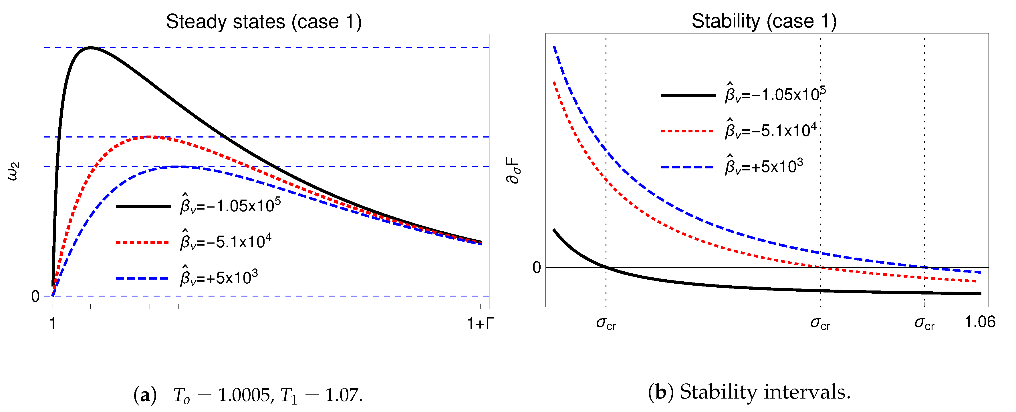
Remark 3.

The critical value (52) tends to $-\infty$ for ${\mathfrak{T}}_o$ going to 1. Thus, we always consider only values of $T_o$ close to but distinct from 1. We notice also that we have to take care of this lower bound only when we consider the case of extraction; that is, ${\widehat{\beta }}_v<0$. For example, for $T_o=1.0005$, we are allowed to consider only ${\widehat{\beta }}_v\gtrsim -2.98\times {10}^6$. On the other hand, from the physical point of view, negative values of ${\omega }_2$, which show natural liquid recharge, are meaningless. Thus, recalling (44), physically meaningful solutions to Equation (35) exist if and only if Ω remains negative. For example, for $T_o=1.0005$ and $\sigma \in (T_o,1+\mathrm{\Gamma })$, the negativity of Equation (50) holds true provided that ${\widehat{\beta }}_v\gtrsim -1.13\times {10}^5$.

In the present case, steady states are described by

$${\omega }_2={\mathfrak{F}}_1(\sigma ,T_o,{\widehat{\beta }}_v),$$

where

$${\mathfrak{F}}_1=-{\left(\mathsf{\Omega }(\sigma ,T_o)\frac{f\left(\sigma \right)}{\sigma }\right)}^{-1}\left(1+\mathrm{\Gamma }-T_1\right)\left(1+{\omega }_1\frac{f\left(\sigma \right)}{\sigma }\right),$$

and $\mathsf{\Omega }$ is given by Equation (50). Recalling Equation (37), we need to study the sign of

$$\frac{\partial F}{\partial \sigma }(\sigma ,{\mathfrak{F}}_1(\sigma ,T_o,{\widehat{\beta }}_v)),$$

by varying both $T_o\in (1,\mathfrak{T}\left(\sigma \right))$ and ${\widehat{\beta }}_v$. Figure 1 provides a synthetic picture of the varying influence of ${\widehat{\beta }}_v$ in determining stable/unstable states.

We have (linearly) stable steady solutions only for $0<{\omega }_2\le {\omega }_{2,\mathrm{cr}}$ and $\sigma \ge {\sigma }_{\mathrm{cr}}$. Figure 1 shows that by decreasing ${\widehat{\beta }}_v$ from positive values (injection) to negative ones (extraction), ${\omega }_{2,\mathrm{cr}}$ increases and ${\sigma }_{\mathrm{cr}}$ decreases (i.e., the physical free boundary shifts towards the top of the reservoir). This means that the liquid region increases due to the augmented meteoric liquid recharge, as physically expected. 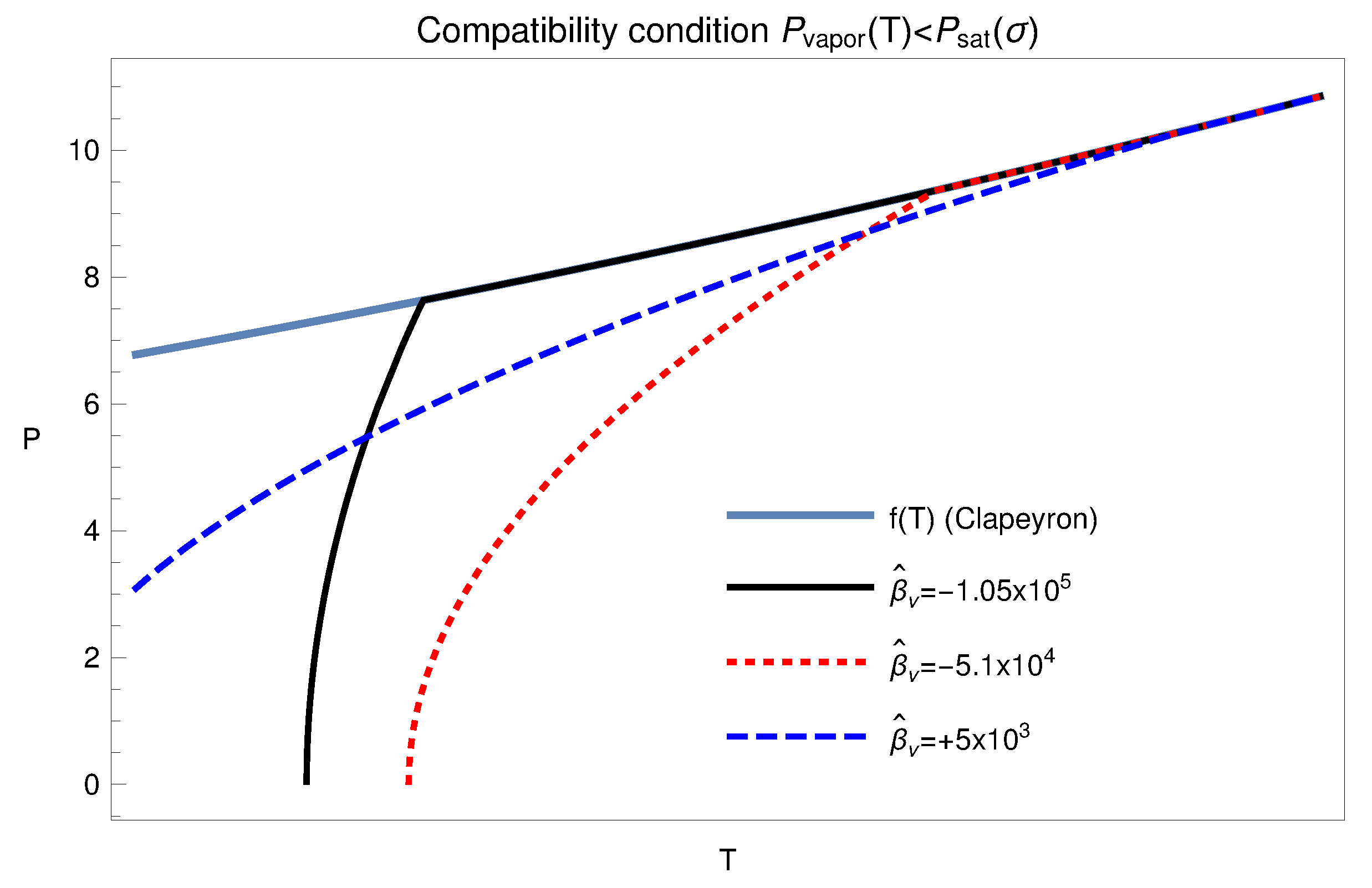Figure 2 shows that solutions represented in Figure 1 satisfy the compatibility condition (18).

4.2. Case 2. Groundwater Recharge Occurring in the Whole Domain and a Single Vapor Extraction/Injection Well

The procedure to obtain the explicit form of $F=0$ is similar to that in Section 4.1, but function $\mathsf{\Omega }$ is more complex. Calculations are presented in such a way to emphasize the differences with respect to Section 4.1.

In this case ${\mathfrak{R}}_{\ell }^{\left(i\right)}=0$, $D_{\ell }$ is given by $1+\mathrm{\Gamma }-\sigma$ (since $T_1=\sigma$), and ${\beta }_v$, given by (30), has the form

$${\beta }_v\left(P,T\right)=B_v\left[1+{\mathfrak{R}}_v\delta \left(T-T_o\right)\right],\mathrm{with}{B}_v=\frac{{\varphi }_o}{{\kappa }_o}\frac{r{\mu }_o{T}_s^3}{{\gamma }^2{P}_s^2}{d}_{v,\mathrm{met}}.$$

(53)

Therefore, Equation (29)$,1$ becomes

$$\frac{\partial }{\partial T}\left[\frac{P}{T}\left(\frac{\partial P}{\partial T}-\eta \frac{P}{T}\right)\right]=-B_v\left[1+{\mathfrak{R}}_v\delta \left(T-T_o\right)\right].$$

Since $B_v{\mathfrak{R}}_v={\widehat{\beta }}_v$, after one integration, we obtain

$$\frac{P}{T}\left(\frac{\partial P}{\partial T}-\eta \frac{P}{T}\right)=-{\widehat{\beta }}_v\theta \left(T-T_o\right)-B_{v}T+C_1,$$

where $C_1$ is the integration constant. Setting again $z=P^2/2$, we get

$$z^{\prime }-2\eta \frac{z}{T}=C_{1}T-{\widehat{\beta }}_{v}T\theta \left(T-T_o\right)-B_v{T}^2,$$

whose general solution is

$$\begin{array}{ccc}z\left(P\right)\hfill & =\underset{\mathrm{case}1}{\underbrace{C_2{T}^{2\eta }-\frac{C_1{T}^2}{2\left(\eta -1\right)}-\frac{{\widehat{\beta }}_v}{2\left(\eta -1\right)}\left[T^{2\eta }{\int }_1^T{\tau }^{2-2\eta }\delta \left(\tau -T_o\right)d\tau -T^2\theta \left(T-T_o\right)\right]}}\hfill & \\ \hfill & +\underset{\mathrm{additional}\mathrm{term}}{\underbrace{\frac{B_v{T}^3}{2\left(\eta -3/2\right)}}},\hfill \end{array}$$

where $C_2$ is the second integration constant. Proceeding as in Section 4.1 (i.e., imposing the boundary conditions in Equations (29)$,2$, and (29)$,3$) we obtain

$$\begin{array}{cccc}{P}^2\left(T\right)\hfill & =\underset{\mathrm{case}1}{\underbrace{T^{2\eta }-A\left(\sigma \right)\left(T^{2\eta }-T^2\right)+{\displaystyle \frac{{\widehat{\beta }}_v}{\eta -1}}\left[\left({\displaystyle \frac{{\sigma }^{2\eta }{T}_o^{2-2\eta }-{\sigma }^2}{{\sigma }^{2\eta }-{\sigma }^2}}\right)\left(T^{2\eta }-T^2\right)\right.}}\hfill & \hfill & \\ \hfill & -\underset{\mathrm{case}1}{\underbrace{\left.{\displaystyle T^{2\eta }{\int }_1^T{\tau }^{2-2\eta }\delta \left(\tau -T_o\right)d\tau +T^2\theta \left(T-T_o\right)}\right]}}\hfill & \hfill & \\ \hfill & +\underset{\mathrm{additional}\mathrm{term}}{\underbrace{{\displaystyle \frac{B_v}{\eta -3/2}}\left[T^3-T^{2\eta }-\left({\displaystyle \frac{{\sigma }^3-{\sigma }^{2\eta }}{{\sigma }^{2\eta }-{\sigma }^2}}\right)\left(T^{2\eta }-T^2\right)\right]}},\hfill & \hfill \end{array}$$

where $A\left(\sigma \right)$ is given by Equation (40), which reduces to Equation (48) when $B_v=0$ and to Equation (39) when ${\widehat{\beta }}_v=0$. Next,

$$\begin{array}{ccc}\hfill {\left.\frac{\partial P}{\partial T}\right|}_{\sigma }& =& \frac{1}{\sqrt{f\left(\sigma \right)}}\left[\eta {\sigma }^{2\eta -1}+A\left(\sigma \right)\left(\sigma -\eta {\sigma }^{2\eta -1}\right)\right]\hfill \\ & +& \frac{{\widehat{\beta }}_v}{\left(\eta -1\right)\sqrt{f\left(\sigma \right)}}\left[\frac{{\sigma }^{2\eta }{T}_o^{2-2\eta }-{\sigma }^2}{{\sigma }^{2\eta }-{\sigma }^2}\left(\eta {\sigma }^{2\eta -1}-\sigma \right)-\left(\eta {\sigma }^{2\eta -1}{T}_o^{2-2\eta }-\sigma \right)\right]\hfill \\ & +& {\displaystyle \frac{B_v}{\left(\eta -3/2\right)\sqrt{f\left(\sigma \right)}}}\left[\frac{3}{2}{\sigma }^2-\eta {\sigma }^{2\eta -1}+\left({\displaystyle \frac{{\sigma }^3-{\sigma }^{2\eta }}{{\sigma }^{2\eta }-{\sigma }^2}}\right)\left(\sigma -\eta {\sigma }^{2\eta -1}\right)\right],\hfill \end{array}$$

which gives (49) when $B_v=0$. Thus, recalling Equations (34), (42) and (50), we have

$$\mathsf{\Omega }={\mathsf{\Omega }}_1\left(\sigma \right)+{\widehat{\beta }}_v\mathcal{G}\left(\sigma ,T_o\right)+B_v\mathcal{H}\left(\sigma \right),$$

where

$$\mathcal{H}\left(\sigma \right)={\displaystyle \frac{1}{\left(\eta -3/2\right)\sqrt{f\left(\sigma \right)}}}\left[\frac{3}{2}{\sigma }^2-\eta {\sigma }^{2\eta -1}+\left({\displaystyle \frac{{\sigma }^3-{\sigma }^{2\eta }}{{\sigma }^{2\eta }-{\sigma }^2}}\right)\left(\sigma -\eta {\sigma }^{2\eta -1}\right)\right].$$

Function H monotonically decreases and is negative. Therefore, $0>\mathcal{H}\left(\sigma \right)>\mathcal{H}(1+\mathrm{\Gamma })\approx -0.015$.

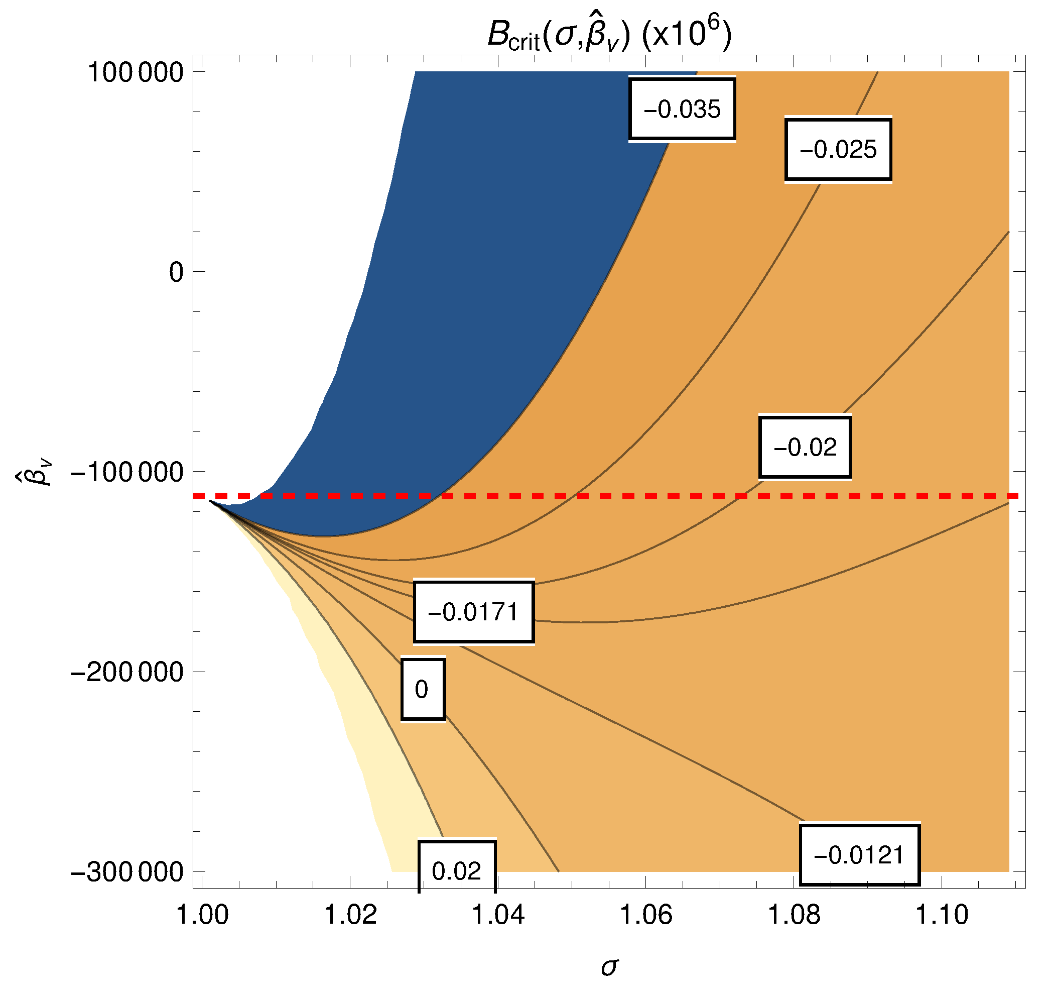
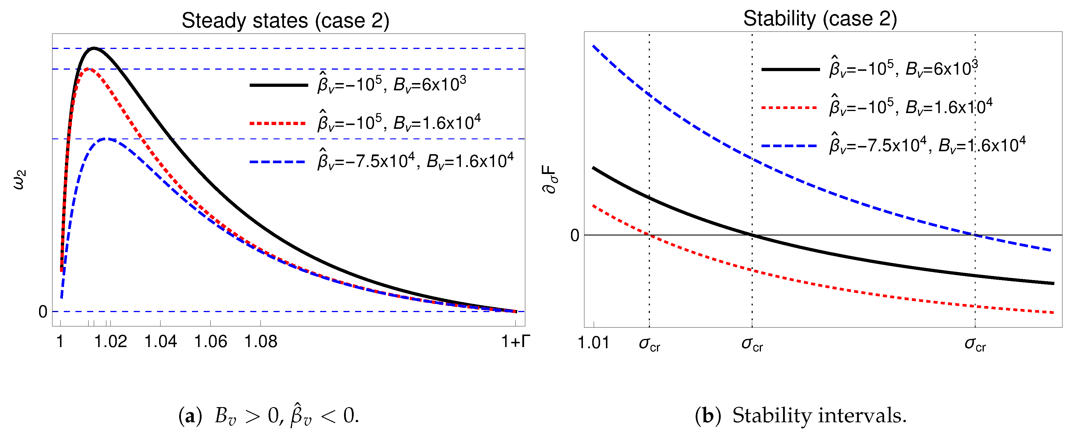
Remark 4.

Recalling what we emphasized in Remark 3, in order to obtain physically meaningful solutions to Equation (38), we need Ω to remain negative when we change ${\widehat{\beta }}_v$ and $B_v$. For fixed $T_o\in (1,{\mathfrak{T}}_o)$ and ${\widehat{\beta }}_v>{\beta }_{\mathrm{cr}}\left({\mathfrak{T}}_o\right)$; this implies

$$B_v>B_{v,\mathrm{cr}}(\sigma ,{\widehat{\beta }}_v,{\mathfrak{T}}_o)=-\frac{{\mathsf{\Omega }}_1\left(\sigma \right)+{\widehat{\beta }}_v\mathcal{G}(\sigma ,{\mathfrak{T}}_o)}{\mathcal{H}\left(\sigma \right)}.$$

(54)

Figure 3 shows the level lines (the white boxes indicate some values) of $B_{v,\mathrm{cr}}$ for all $\sigma \in (1,1+\mathrm{\Gamma })$ and ${\widehat{\beta }}_v$ varying over 10 orders of magnitude from negative to positive values, when ${\mathfrak{T}}_o=1.0005$. To handle a specific case, one fixes ${\widehat{\beta }}_v>{\beta }_{\mathrm{cr}}\left({\mathfrak{T}}_o\right)$ and uses $\underset{\sigma >T_o}{sup}{B}_{\mathrm{cr}}(\sigma ,{\widehat{\beta }}_v,{\mathfrak{T}}_o)$ as a critical value. We notice that only non-negative values of $B_v$, which is the meteoric recharge, are of physical interest; when ${\widehat{\beta }}_v\ge 0$, $\underset{\sigma >T_o}{sup}{B}_{v,\mathrm{cr}}$ is negative (≈$-1.9\times {10}^4$) and Equation (54) does not need to be invoked. For ${\widehat{\beta }}_v$ negative (extraction), $\underset{\sigma >T_o}{sup}{B}_{v,\mathrm{cr}}$ continues to be negative as long as ${\widehat{\beta }}_v>-1.13\times {10}^5$. Thus in our simulations, we always keep ${\widehat{\beta }}_v\ge -{10}^5$.

We have stable steady solutions only for $0<{\omega }_2\le {\omega }_{2,\mathrm{cr}}$ and $\sigma \ge {\sigma }_{\mathrm{cr}}$. Figure 4 shows that by increasing ${\widehat{\beta }}_v$ and keeping $B_v>0$ fixed, ${\omega }_{2,\mathrm{cr}}$ decreases while ${\sigma }_{\mathrm{cr}}$ increases. On the contrary, increasing $B_v$ and keeping ${\widehat{\beta }}_v<0$ fixed causes ${\omega }_{2,\mathrm{cr}}$ to decrease and ${\sigma }_{\mathrm{cr}}$ to decrease. This behavior also agrees with physical expectations. 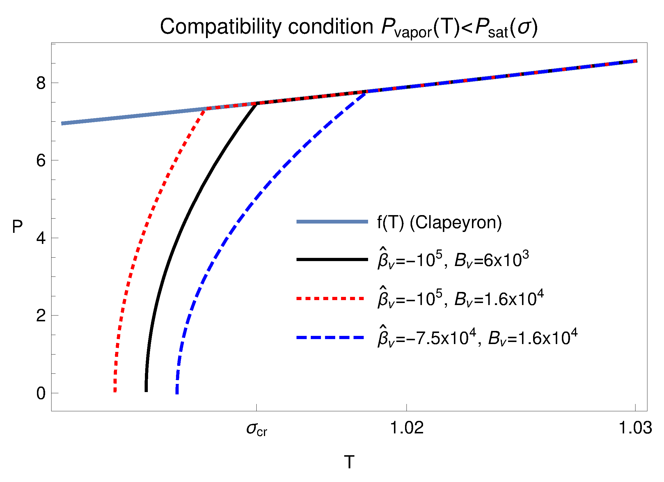Indeed, increasing the vapor extraction with a fixed vapor recharge (i.e., from the blue curve to the red one) implies that ${\sigma }_{\mathrm{cr}}$ decreases, and the liquid natural recharge needs to be adjusted at higher rates to maintain stability. On the other hand, a fixed extraction rate and a decreasing natural vapor recharge (i.e., from the red curve to the black one) imply that, to maintain stability, the liquid natural recharge must increase and the critical interface must increase. Figure 5 shows that the compatibility condition (18) is satisfied.

4.3. Case 3. Recharge Due to a Single Injection Well Localized in the Liquid Domain

In this case, ${\beta }_v=0$ and $d_{\ell ,\mathrm{met}}=0$, so that Equation (26) can be rewritten as

$$D_{\ell }=\frac{d_{\ell ,\mathrm{inj}}{T}_s}{\gamma }$$

since ${\tilde{D}}_{\ell }=1$, which is the injection well located in the liquid domain. The solution to (29) is given by Equation (39), and so F as defined by Equation (33) becomes

$$\begin{array}{ccc}\hfill F\left(\sigma \right)& =& \left({\displaystyle \frac{d_{\ell ,\mathrm{inj}}{T}_s}{\gamma }}\right)\left[1+\left({\displaystyle \frac{P_s}{r{T}_s{\rho }_{\ell ,o}}}\right)h\left(\sigma \right)\right]\hfill \\ \\ & +& \left({\displaystyle \frac{{\kappa }_o{P}_s^2\gamma }{{\varphi }_{o}r{\rho }_{\ell ,o}{\mu }_o{T}_s^2}}\right){\displaystyle \frac{\kappa \left(\sigma \right)h\left(\sigma \right)}{\varphi \left(\sigma \right)\mu \left(f\left(\tilde{\sigma }\right),\tilde{\sigma }\right)}}{\mathsf{\Omega }}_1\left(\sigma \right)\hfill \end{array}$$

with ${\mathsf{\Omega }}_1\left(\sigma \right)$ given by Equation (42). Thus, setting

$${\omega }_3=\frac{{\kappa }_o{P}_s^2{\gamma }^2}{{\varphi }_{o}r{\rho }_{\ell ,o}{\mu }_o{T}_s^3{d}_{\ell ,\mathrm{inj}}},$$

the function F acquires this form:

$$F\left(\sigma \right)=1+{\omega }_1\frac{f\left(\sigma \right)}{\sigma }+{\omega }_3\frac{f\left(\sigma \right)}{\sigma }{\mathsf{\Omega }}_1\left(\sigma \right),$$

(55)

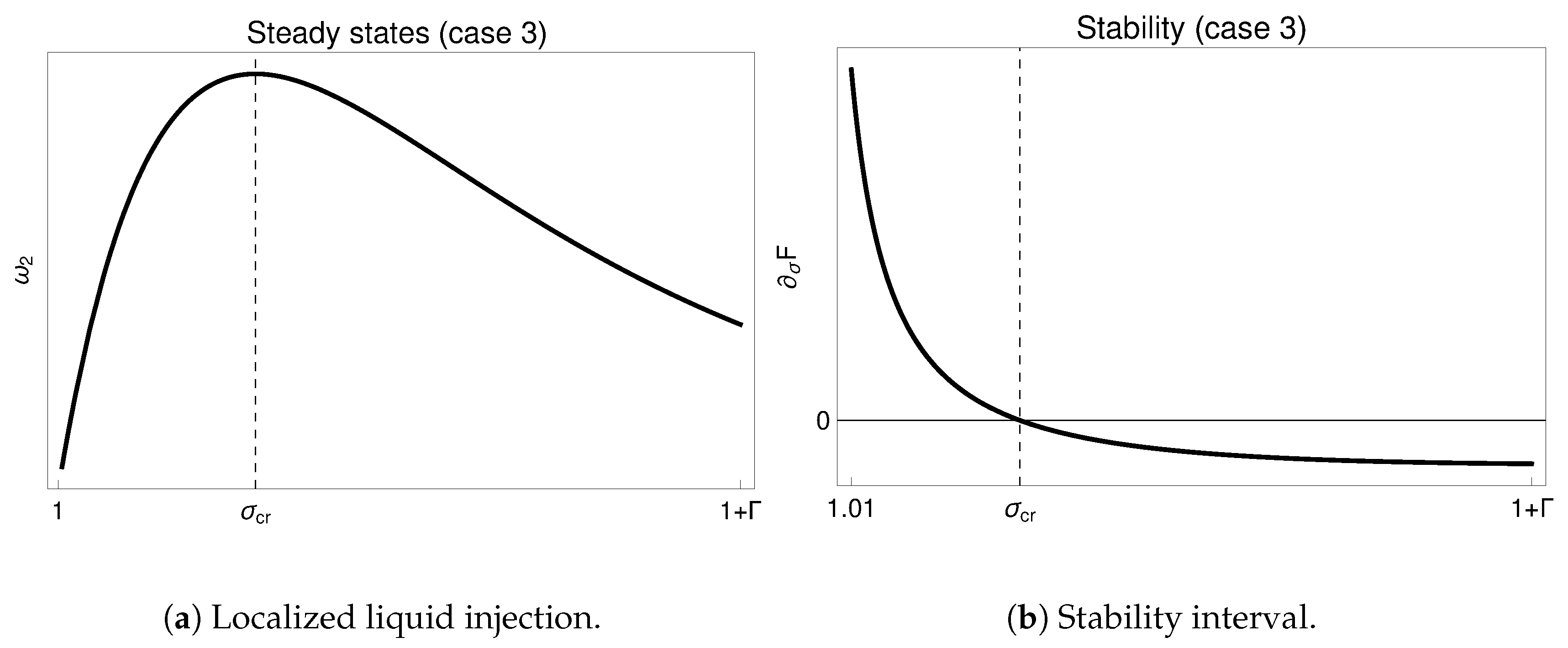
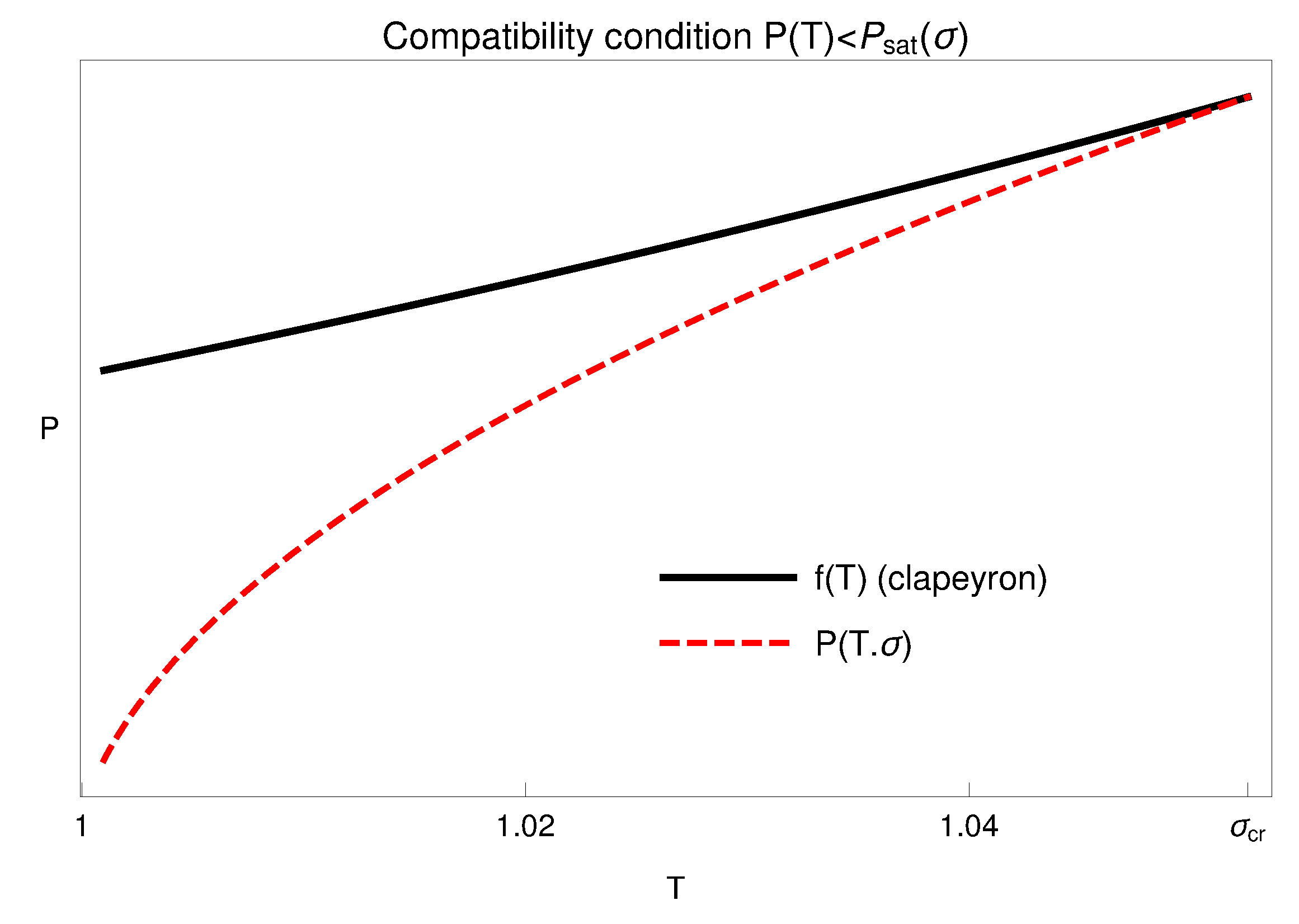
where ${\omega }_1$ has been defined in Equation (45)$,1$ without any constraints on ${\omega }_3$ since ${\mathsf{\Omega }}_1$ is always strictly negative. Figure 6 shows the stable steady states in the present case and Figure 7 shows that the compatibility condition (18) is fulfilled.

5. Sustainability of Equilibria and Re-Injection

The main environmental and industrial issue concerning a geothermal field is the long-term sustainability of its power production capability. Since the middle of the last century, this question has been deeply discussed in the specialized literature [40,45,47,49,50], and the primary role of re-injection has been clearly emphasized. It is interesting to express the equilibrium conditions investigated in this study in dimensional variables and to compare them with some historical field data referring to the Larderello reservoir. Due to the severe approximations considered, such a comparison does not have any specific intention but to meet, at least, the order of magnitude of the most significant and available data.

An estimate of the volume $V_{\mathrm{field}}$ of the Larderello reservoir [10,11,14] is about $8\times {10}^{11}{\mathrm{m}}^3$. Assuming the porosity of Table 1, the volume $V_{\mathrm{fluid}}$ of fluid in the reservoir is on the order of $1.6\times {10}^{10}{\mathrm{m}}^3$. The meteoric recharge from the shallow aquifer surrounding the reservoir is not constant in time; it depends on a variety of factors and can only be roughly estimated [40]. The rate of steam extraction $Q_{\mathrm{extr}}$ has changed considerably during the last decades; for example, it was about 300 $\mathrm{k}\mathrm{g}/\mathrm{s}$ in the 1950s and declined to about 150 $\mathrm{k}\mathrm{g}/\mathrm{s}$ in the 1980s [11]. Precise historical series are available from ENEL, the company holding the rights of exploitation of the Larderello geothermal fields [2]. In the 1990s, the natural recharge $Q_{\mathrm{nat}}$ from the shallow aquifers in the area was estimated to be about one quarter of the extraction rate $Q_{\mathrm{extr}}$ [40]. Due to re-injection, it is likely that the ratio of extraction/natural recharge has not changed very much [10,13]. To solve these ürpnöe,s, we assume $Q_{\mathrm{nat}}=0.25Q_{\mathrm{extr}}$ at any time. Then, we define

$$Q_{\mathrm{field}}\left(t\right)=-Q_{\mathrm{extr}}\left(t\right)+Q_{\mathrm{nat}}\left(t\right)=-0.75Q_{\mathrm{extr}}\left(t\right)$$

(56)

Consider, now, “case 2” as discussed in Section 4.2. According to the model, the total discharge per unit volume (that is, in $\mathrm{k}\mathrm{g}/\left({\mathrm{m}}^3\mathrm{s}\right)$) is given by

$$q_{\mathrm{model}}={\rho }_{\ell }{d}_{\ell ,\mathrm{met}}+d_{v,\mathrm{met}}+d_{v,\mathrm{inj}},$$

(57)

where $d_{\ell ,\mathrm{met}}$, $d_{v,\mathrm{met}}$ and $d_{v,\mathrm{inj}}$ are determined by the dimensionless parameters ${\omega }_2$, ${\widehat{\beta }}_v$, and $B_v$ through (45)$,2$, (46)$,2$, and (53)$,2$, i.e.,

$$d_{\ell ,\mathrm{met}}=C_1{\omega }_2^{-1},d_{v,\mathrm{met}}=C_2{B}_v,d_{v,\mathrm{inj}}=C_2{\widehat{\beta }}_v,$$

(58)

where, by using data from Table 1,

$$C_1=\frac{{\kappa }_o{P}_s^2{\gamma }^2}{{\varphi }_{o}r{\rho }_{\ell }{\mu }_o{T}_s^3}\approx 2.6\times {10}^{-13}{\mathrm{s}}^{-1},C_2={\rho }_{\ell }{C}_1\approx 2.1\times {10}^{-10}\mathrm{k}\mathrm{g}{\mathrm{m}}^{-3}{\mathrm{s}}^{-1}.$$

(59)

For fixed values of ${\widehat{\beta }}_v<0$ and $B_v>0$, any stable steady state is represented by a point $(\sigma ,{\omega }_2)$, with $0<{\omega }_2<{\omega }_{\mathrm{crit}}$ and $\sigma >{\sigma }_{\mathrm{crit}}$, on the curve ${\omega }_2=\mathfrak{F}(\sigma ;{\widehat{\beta }}_v,B_v)$. Therefore the real location of the interface depends upon the effective value of ${\omega }_2$. At any time during the evolution of the reservoir, we can relate $q_{\mathrm{model}}$ with $Q_{\mathrm{field}}$ since

$$Q_{\mathrm{field}}=q_{\mathrm{model}}\times V_{\mathrm{fluid}},$$

(60)

and exploiting (57) and (58), we have

$$\frac{Q_{\mathrm{field}}}{C_2{V}_{\mathrm{fluid}}}={\mathfrak{F}}^{-1}(\sigma ;{\widehat{\beta }}_v,B_v)+{\widehat{\beta }}_v+B,$$

(61)

where $C_2$ is given by Equation (59). To evaluate the left-hand side of Equation (61), we extracted some data from the historical series reported by Pallotta [2]. Notice that

$$\frac{Q_{\mathrm{field}}}{V_{\mathrm{fluid}}}\approx -{10}^{-8}\mathrm{k}\mathrm{g}/\left({\mathrm{m}}^3\mathrm{s}\right),$$

so that $Q_{\mathrm{field}}/\left(C_2{V}_{\mathrm{fluid}}\right)=\mathcal{O}\left({10}^2\right)$ (see

Table 2. Production history of the Larderello field from 1960 to 2015. Artificial re-injection started in 1975.

Year	${\mathit{Q}}_{\mathbf{extr}}$ (kg/s)	${\mathit{Q}}_{\mathbf{field}}/\left({\mathit{C}}_2{\mathit{V}}_{\mathbf{fluid}}\right)$
1960	412	−92
1970	287	−64
1975	241	−54
1985	255	−57
1995	266	−59
2000	275	−62
2010	294	−66
2015	315	−69

). Using $B_v$ and ${\widehat{\beta }}_v$ as free parameters, Equation (61) and Table 2 provide a simple criterion to relate the Larderello field data with the equilibrium interface. For example, selecting $Q_{\mathrm{field}}/\left(C_2{V}_{\mathrm{fluid}}\right)=-69$ (the 2015 datum), ${\widehat{\beta }}_v=-7.5\times {10}^4$, $B_v=1.6\times {10}^4$, Equation (61) is fulfilled with $\sigma \approx 1.088$, (i.e., $s\approx -2220\mathrm{m}$), which is stable because, in case 2, with this choice of parameters, all interfaces $\sigma >1.018$ are stable (see Figure 4). If we keep $B_v=1.6\times {10}^4$ and decrease ${\widehat{\beta }}_v$ up to $-1.2\times {10}^5$, the new stable position of the interface is around $-2560\mathrm{m}$. According to Figures 22 and 23 in [10], at a depth of about $-2000$ m, the fluid pressure in 2010 was 10 bar and the temperature was around 550 K. The real fluid present in the reservoir is not pure water but a complex mixture of water, carbon dioxide and several other chemical components with a great variability of molar fractions. Even for a simple binary water–carbon dioxide system, the estimated saturation pressure would be greatly above the values reported in [10]. It must be emphasized, however, that for a real geothermal fluid, precise indications about the vapor saturation pressure are still lacking, and only some models are supplied [51,52,53]. This suggests, in any event, that for the Larderello field, the vapor/liquid interface must be deeper than $-2000$ m a.s.l. [30]. All this considered, our model, besides its indisputable simplicity and considerable approximations, locates the interface below the above limit provided that the parameters are selected consistently with the field data. This is certainly a very encouraging result. Nomenclature and other symbol definitions can be found in

Table 3. Nomenclature and other symbol definitions.

Symbol	Description	Units	First Used in Formula
L	Reservoir thickness	$\mathrm{m}$	(2)
v	Vapor velocity	$\mathrm{m}{\mathrm{s}}^{-1}$	(3)
$v_{\ell }$	Liquid velocity	$\mathrm{m}{\mathrm{s}}^{-1}$	(8)
$d_v$	Vapor density rate	$\mathrm{k}\mathrm{g}{\mathrm{m}}^{-3}{\mathrm{s}}^{-1}$	(4)
$d_{\ell }$	Liquid water source density rate	${\mathrm{s}}^{-1}$	(8)
$\delta$	Dirac delta	-	(4)
$D_{\ell }$	Total liquid recharge rate	$\mathrm{m}{\mathrm{s}}^{-1}$	(12)
$P^{*}$	Clapeyron pressure	$\mathrm{Pa}$	(15)
${\beta }_v$	Pressure source term	-	(30)
$Q_{\mathrm{field}}$	Reservoir flow rate	$\mathrm{k}\mathrm{g}{\mathrm{s}}^{-1}$	(56)
$q_{\mathrm{mod}}$	Total discharge per unit volume	$\mathrm{k}\mathrm{g}{\mathrm{m}}^{-3}{\mathrm{s}}^{-1}$	(57)
$\sigma$	Liquid/vapor interface	-	(22)
N	Number of injection heads	-	(4)
$P_{\mathrm{inj}}$	Re-injection pressure	$\mathrm{Pa}$	(4)
$d_{\ell ,\mathrm{inj}}^{\left(i\right)}$	i-th re-injection rate order of magnitude	$\mathrm{m}{\mathrm{s}}^{-1}$	(13)
${\mathfrak{R}}_{\ell }^{\left(i\right)}$	i-th liquid injection to meteoric rate ratio	-	(28)
${\mathfrak{R}}_v^{\left(i\right)}$	i-th vapor injection to meteoric rate ratio	-	(31)
$V_{\mathrm{field}}$	Reservoir volume	${\mathrm{m}}^3$	(60)
$T_o$	Injection well depth	-	(47)

.

6. Conclusions

The main conclusion of our investigation is that stable stationary states of the liquid/vapor interface are possible either with liquid or vapor recharge combined with vapor extraction. The main parameters ${\omega }_2$ (natural liquid recharge), ${\beta }_v<0$ (vapor extraction) and $B_v>0$ (vapor meteoric recharge) need to be combined conveniently to maintain a stable interface. Increasing the vapor extraction moves the interface towards the bottom of the reservoir, which at the limit is shown to be increasingly vapor-dominated. Interestingly, stable interfaces can generally be obtained only if ${\omega }_2$ is less than a critical value; that is, only if the natural liquid recharge is sufficiently large.

The results obtained considering uniform porosity and permeability provide a good qualitative description of the possible steady configurations of a vapor-dominated basin such as Larderello.

An important characteristic of the model is that stationary stable states are compatible with the presence of natural and artificial recharging mechanisms. Such a conclusion agrees with the results of other geological studies [18], despite the drastic simplifications introduced in our model: 1D geometry, an absence of chemicals dissolved in water and uniform geological parameters (which, in a real geothermal field, are far from being homogeneous and may change significantly due to local temperature and pressure). The differential Equation (19), 4, has been proven to be quite satisfactory for modeling the vapor drawdown from a reservoir and for recharging from both aquifers and injection wells. We also think that our analysis is likely to produce physically meaningful results also for equilibrium configurations of water-dominated fields. In conclusion, we believe that, despite the many simplifications made in the model, this study can be an useful step towards improving our understanding of the dynamics of geothermal fields.