Article

Effect of Demand Side Management on the Operation of PV-Integrated Distribution Systems

1
Department of Electrical and Computer Engineering, Birzeit University, Birzeit PO Box 14, Palestine
2
Dipartimento di Ingegneria, Università di Palermo, 90128 Palermo, Italy
*
Author to whom correspondence should be addressed.
Appl. Sci. 2020, 10(21), 7551; https://doi.org/10.3390/app10217551
Submission received: 10 September 2020 / Revised: 22 October 2020 / Accepted: 23 October 2020 / Published: 27 October 2020
(This article belongs to the Section Electrical, Electronics and Communications Engineering)

Abstract

:
In this new era of high electrical energy dependency, electrical energy must be abundant and reliable, thus smart grids are conducted to deliver load demands. Hence, smart grids are implemented alongside distributed generation of renewable energies to increase the reliability and controllability of the grid, but, with the very volatile nature of the Distributed Generation (DG), Demand Side Management (DSM) helps monitor and control the load shape of the consumed power. The interaction of DSM with the grid provides a wide range of mutual benefits to the user, the utility and the market. DSM methodologies such as Conservation Voltage Reduction (CVR) and Direct Load Control (DLC) collaborate in the reduction of plant generation and reciprocally to the comprehensive cost. The aim of this paper is to investigate the effects caused by the implementation of DSM on the operation of PV-integrated distribution systems. The algorithms of CVR, DLC and the combination of CVR and DLC were implemented using OpenDSS and MATLAB. The effectiveness of the aforementioned schemes was verified on IEEE 30-Bus test system. Various possible integration scenarios between Photovoltaic (PV) and DSM schemes are illustrated. The optimal integration of such schemes constraining the reduction of energy consumed by the user and utility is presented. The results show that the implemented DSM algorithms provide a noticeable reduction in energy losses and reduction in consumed energy.

1. Introduction

With the fast-paced technological advancement of the twenty-first century, electrical demand is constantly increasing. This is mainly due to the exponential growth of the human population, the need for more electrical appliances in every household and the constantly developing industry. Conventional power grids suffer from many disadvantages, such as low reliability and security and higher losses compared to smart grids, which are more commonly used nowadays. Smart grids offer many advantages; along with their higher reliability and security, they tend to be more environmentally friendly, more economical and safer [1,2,3,4]. One of the early solutions to the problem of increasing electrical demand was the implementation of DG, which, alongside smart grids, can improve the reliability of the network drastically, offer reactive power control, etc. [2,4]. DG can be classified according to the technological point of view into traditional and nontraditional technologies. Traditional or nonrenewable technologies include internal combustion engines, combined cycles, combustion turbines and micro-turbines. Renewable technologies include solar, wind, geothermal, ocean and fuel cell [5,6]. Solar energy is one of the most significant and attractive types of renewable energies. The main solar power type is photovoltaic (PV). The PV system employs PV cells to convert solar energy to electrical power. The PV cell is an electrical device that produces electricity directly from the sunlight [7]. When a power network employs smart grid technologies with the presence of PV system, the behavior of the network becomes very dependent on the weather and other parameters, thus it becomes unpredictable. DSM can be used in smart grids to complement the unpredictability of the DGs by reducing energy costs and consumption, leading to a more controllable network [1]. DSM has established a new way for energy saving at demand/load side. It has become a sustainable resource for accomplishing energy conservation and environmental protection as well as economical business profit [1,8].
The integration of DSM is not a simple process. Many barriers are faced that include the changes on the system’s protection, the implementation of various DG types and interfacing with communication systems during severe weather cases and natural disasters. This means a new set of regulations is required for a successful, reliable and efficient integration of DSM [8].
Recent advancement in research and development on DSM technologies has created an important role for DSM in the future energy distribution due to its improved performance and flexibility to achieve higher energy efficiency and reduced energy cost [9,10,11,12,13,14]. DSM techniques have attracted the interest of many researchers and several review papers have been published on this subject. The authors of [10] aggregated the expressions and methodologies about DSM subjects and presented explicit definitions of the relevant concepts. In addition, this review paper introduces comprehensive categorization of DSM strategies and proposes a theoretical framework aims to unify the terminology, concepts and modalities. The authors of [11] revisited and scrutinized the strategies of DSM and discussed the challenges of DSM implementation and their associated solutions. The authors of [12] presented a systematic review of supply and demand side optimal load scheduling in a smart grid environment. A review of peak load shaving and Demand Response (DR) strategies, challenges and opportunities is addressed in [13]. Jabir et al. [14] presented a review of the impacts of DSM on electrical power systems. The potential benefits derived by implementing DSM are also discussed. Based on the above literature review, Table 1 shows the summary of some DSM implementations.
Several studies have presented algorithms in the field of DLC and CVR. Macedo et al. [25] proposed monitoring load curves of different houses in the same area to come up with a schedule for managing the utility by employing an artificial neural network and then using DLC. Mahmood et al. [26] proposed maintaining low energy consumption and peak load reduction by using smart metering and automatically controlling home appliances. In this scheme, users’ control units share information regarding energy consumption; the final results show a reduction in peak demand and energy costs. Lopez et al. [27] proposed a model to optimize energy consumption using load shifting by means of electric vehicles and other storage systems, as well as with the help of hourly pricing. Samadi et al. [28] proposed the integration of users to provide information relating to their energy demand patterns, which leads to building utility functions for each user. They then used a mechanism to maximize these utility functions while minimizing costs with the implementation of time-of-use pricing. The authors of [29] proposed to minimize the peak demand on an hourly basis to obtain a balanced daily schedule. They shifted shiftable appliances using the individual power consumption patterns of users and real-time-pricing with integer linear programming. Mohsenian-Rad et al. [30] discussed smart home appliances usage scheduled according to an optimization algorithm that includes PV panels acting as power supply while using DLC. Mohsenian-Rad et al. [23] discussed a scheduling game, where the players are the consumers and their strategies are daily usage of house appliances. The technique uses the Nash equilibrium. Klaić et al. [31] emphasized the positive effects of PV panels at consumer side on peak demand hours and proposed a direct load control over air conditions on a radial residential network. Monyeia et al. [32] investigated the implementation of DSM in South Africa by controlling clothes washers and dryers considering 100%, 50% and 30% consumer participation. Using a modified genetic algorithm, they showed how electricity bills can be reduced in all three cases by using DLC. Bhattarai et al. [33] investigated a control scheme for implementing demand response in a system with three affecting sides: distribution system operators, aggregators and demand response resources. Three control levels were proposed that change frequency and voltage depending on the threshold-controllable loads. Beal et al. [34] developed load grouping based on power color algorithm of stochastic-constraint satisfaction. This method divides loads into groups of different colors based on how flexible these loads are in terms of shutting the loads off at a given time. Then, DLC was implemented while considering the aforementioned algorithm.
The benefits of CVR in terms of energy savings and loss reduction have been studied [35,36]. The authors of [37] showed that CVR provides energy and economic savings for the utility and the customer. Different implementation methods of CVR are described in [38]. In [39], the authors presented a comprehensive analysis of the possible impacts of different penetration levels of DG on voltage profiles in low-voltage secondary distribution networks. Bag et al. [40] proposed to implement DSM through load curtailment of constant impedance loads on a radial network by using CVR. The method simulated intended to operate substations at rated voltage and then find the optimal capacitor position (OCP) to keep different bus voltages near their lower voltage limit (the lowest allowed voltage by energy authority regulations); this reduction in bus voltage would lead to lowering the demand; by taking the OCP, the technical losses in the network are lower. A field-validated load model for the calculation of the energy conservation gains due to CVR in secondary networks is presented in [41].
The aforementioned review shows that researchers have focused on the implementation of each DSM technique individually; in addition, some researchers have investigated the existence of DSM lacking the presence of intermittent distributed energy resources and its impact when applying DLC and CVR separately. On the other hand, many researchers have proposed appealing results and methods for DLC and CVR, but these methods have not investigated the periods of the day and the commutation between the dominance of DLC and CVR techniques to achieve the maximum reduction of consumed energy. The main contribution of this paper is to investigate the effects of implementing the algorithms of CVR and DLC on the operation of PV-integrated distribution systems. Various possible integration scenarios between PV, CVR and DLC are illustrated. The use of both CVR and DLC is suggested and tested based on two methods: the first method consists of running CVR and DLC proposed algorithm during the entire day (24-h), while the second method implements CVR during low peak demand periods and DLC during high peak demand periods. Moreover, the optimal integration of such schemes constraining the reduction of energy consumed by the user and utility is presented. This paper also shows how the integration of PV can alleviate voltage violations when CVR is applied as well as how the combination of CVR, DLC and PV allows further increasing in the energy savings.
This paper is organized into four sections and the rest of the paper is prepared as follows: Section 2 gives an introduction about DSM technology, including a brief description of DSM techniques. Moreover, the CVR and DLC algorithms and implementation are addressed in this section. Section 3 presents simulation results and the verification of the proposed algorithms. In addition, in this section, different scenarios are established by the commutation between the existence of DG, CVR and DLC. The last section concludes the work presented.

2. Demand Side Management

The term demand side management is the result of a logical evolution of planning processes used by the utilities. Different regions have their own technical challenges, which means they have a different emphasis in terms of what benefits and functionality DSM can deliver over and above that of their existing power system. Different concepts make different assumptions with varying details outlining its smart grid concept. Although DSM does not have a single clear international definition, there are some known definitions used for the DSM [42,43,44]. The following description presents the most detailed and comprehensive definition of DSM: “The planning, implementation, and monitoring of those utility activities designed to influence customer use of electricity in ways that will produce desired changes in the utility’s load shape, i.e., changes in the time pattern and magnitude of a utility’s load. Utility programs falling under the umbrella of demand-side management include: load management, new uses, strategic conservation, electrification, customer generation, and adjustments in market share” [42].

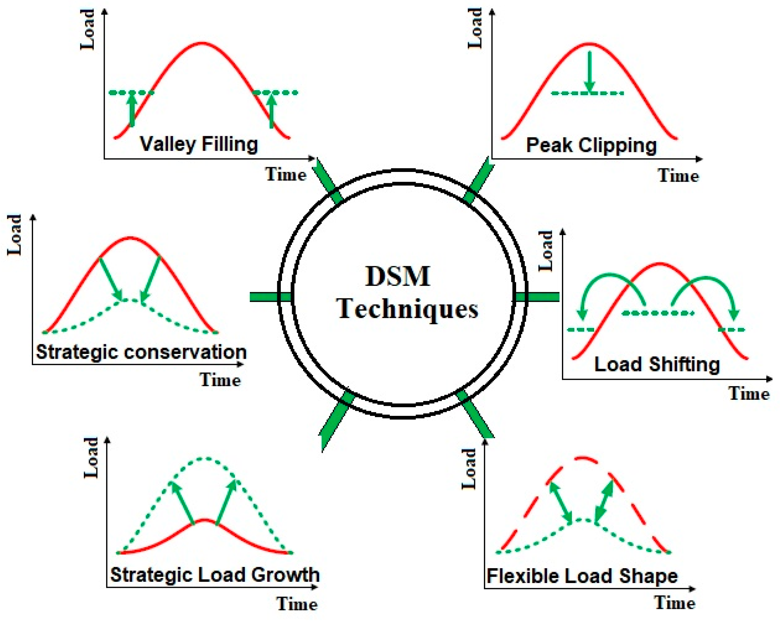
2.1. General Overview of DSM Techniques

With the ever-growing demand globally, investments on new generation capacity must be made everywhere. However, one can cut these investments by implementing DSM, which can be done through a set of actions that reshape the load curve. Figure 1 defines DSM objectives. The main three actions are peak clipping, valley filling and load shifting. Peak clipping means reducing the load demand at high demand periods. This can be achieved by turning off particular consumer equipment and distributed generation. Valley filling encourages consumers to raise their energy demand at times of low demand, during which the cost of energy is cheaper. Load shifting results in shiftable loads being shifted from peak demand periods to lower demand periods. The total consumption stays the same. Strategic conservation decreases the overall seasonal consumption of energy, primarily by reducing energy wastage, thus increasing the efficiency of the system. Strategic load growth results in an overall increase of seasonal energy consumption. The dealership deploys intelligent systems, energy-efficient devices and more competitive sources of energy for achieving the objective. Flexible modeling involves a contract between the consumer and the concessionaire. With the help of load-limiting devices, the energy consumed by the consumer at a given time is limited to a certain value that cannot be exceeded [45,46,47,48].

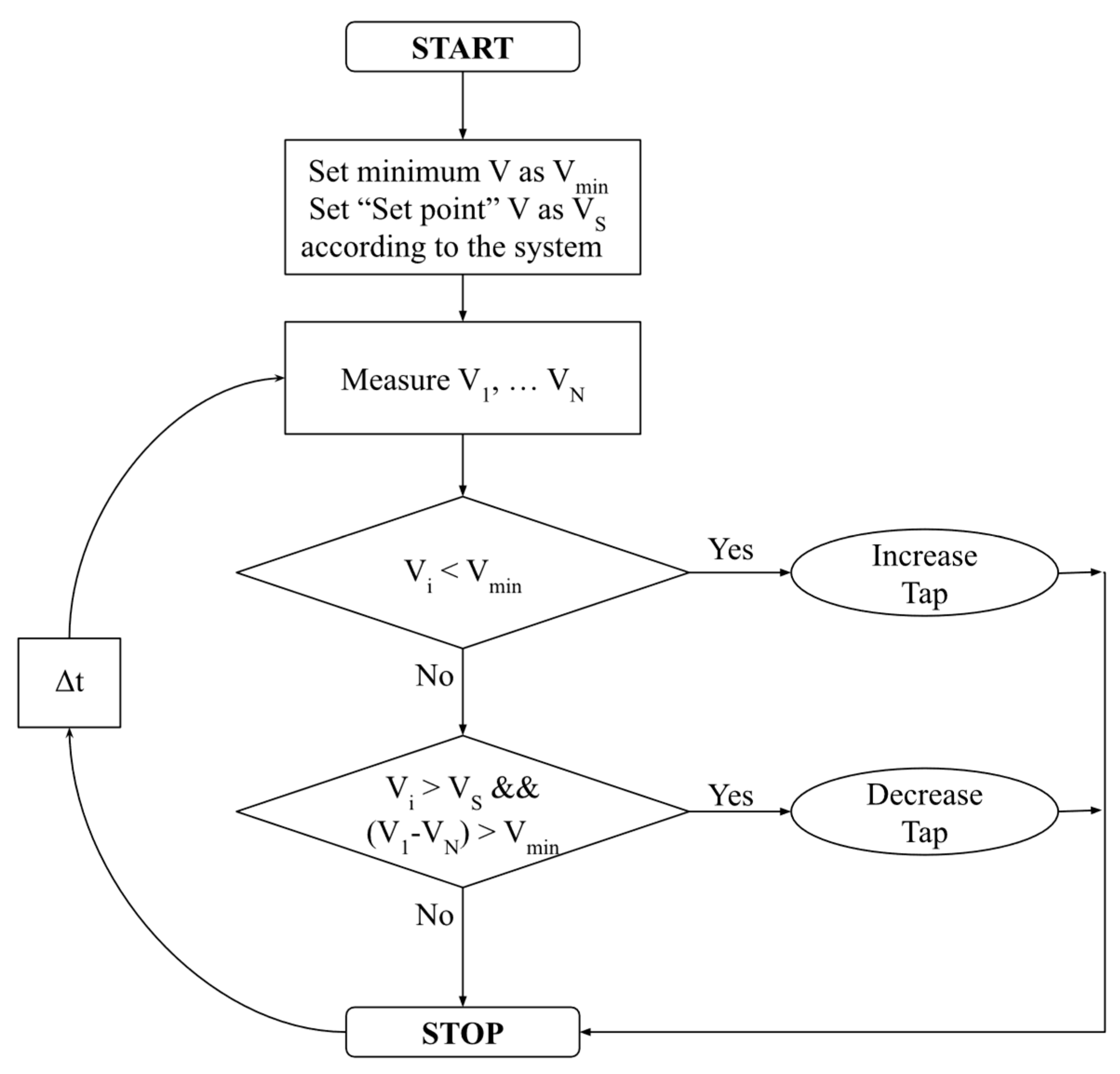
2.2. Implementation of CVR Algorithm

In the CVR method, DSM is implemented through the action of load curtailment. The goal of CVR is to reduce the voltage at consumer side while maintaining the minimum allowable voltage. The flowchart in Figure 2 takes an assigned Voltage Set Point (Vs) and the minimum allowable voltage (Vmin) according to voltage standards [49,50,51] and keeps measuring voltages at customer buses and then increases or decreases the taps of tap-changing transformers until all the bus voltages lie between Vmin and Vs. Δt stands for the time difference between different voltage measurements.

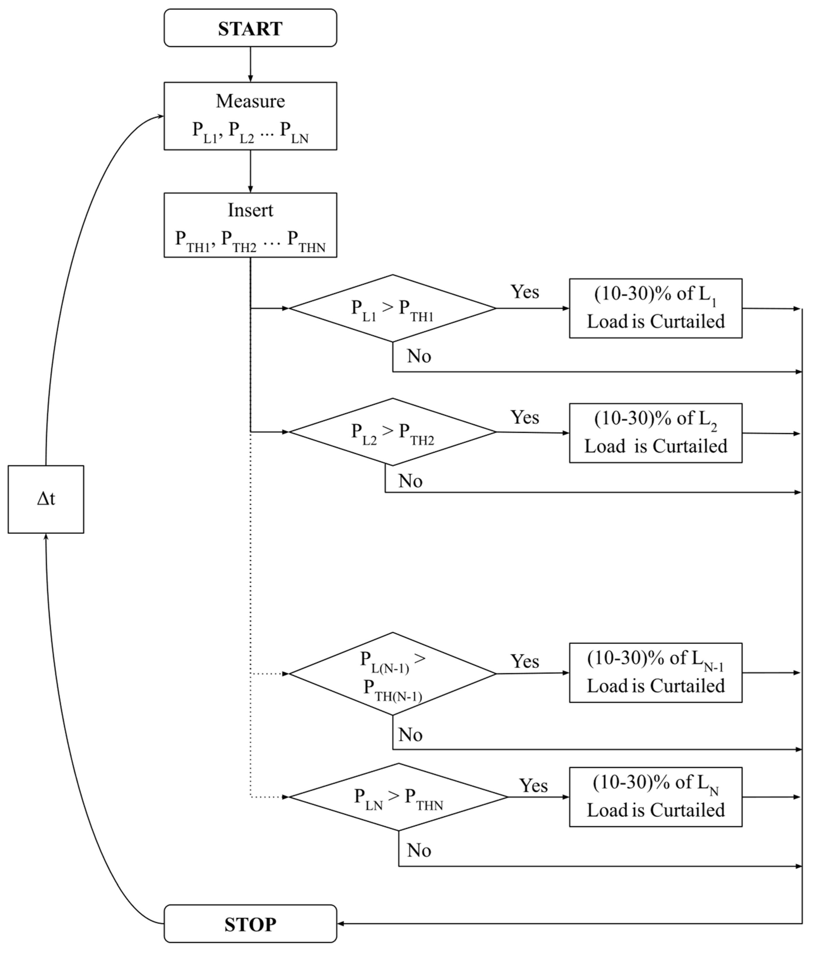
2.3. Implementation of DLC Algorithm

In the DLC method, DSM is implemented through the action of partial load curtailment. The goal of DLC is to reduce the power consumed when high consumption is experienced by the user. The flowchart in Figure 3 measures the power of each load. It starts by comparing each load with its pre-declared threshold (PTH) during an interval of (Δt) 30 min. Once the consumed power by the loads/users exceeds this threshold, load control is taken into place. DLC curtails 10–30% of the load, maintaining the loads with the highest priority active. Finally, if consumption drops below PTH, the algorithm automatically connects the curtailed percentage back to the load.

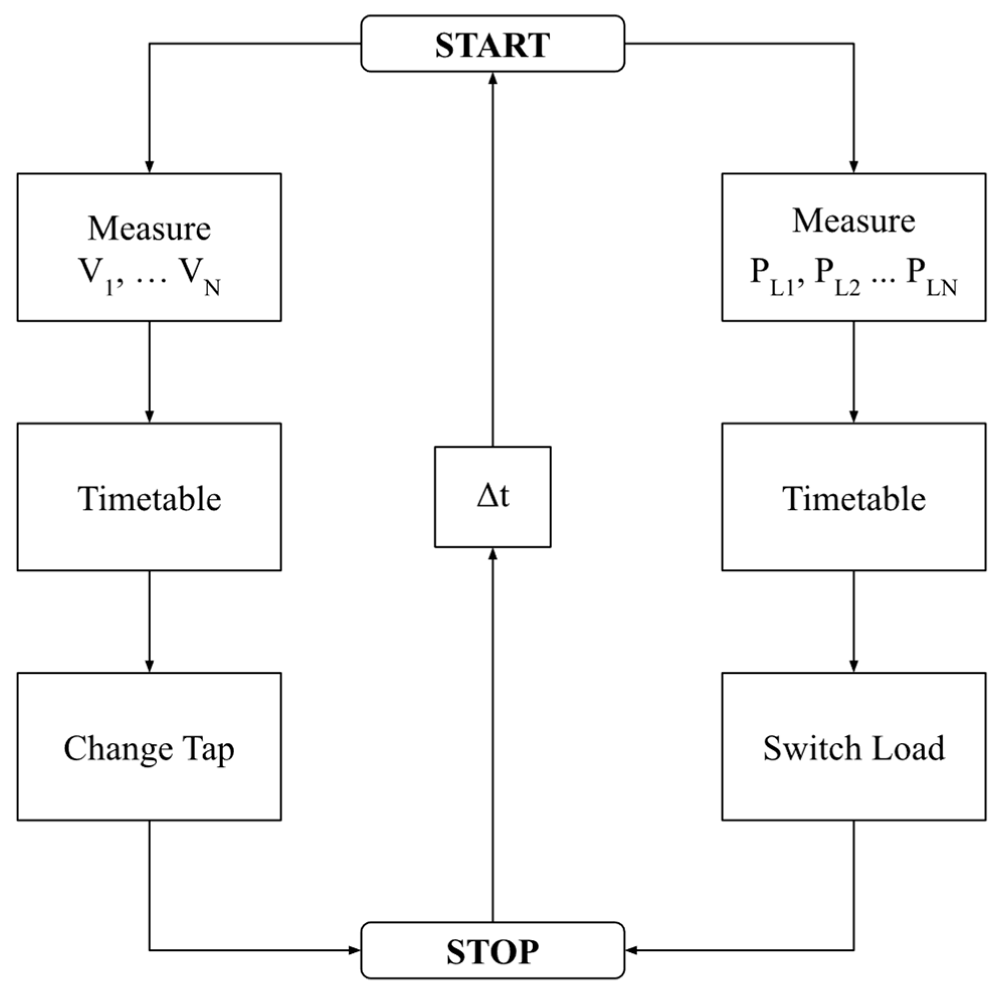
2.4. Implementation of the Proposed Algorithm

The load profile varies during the day, and the best load shape can be achieved by executing an adaptive algorithm that chooses appropriate DSM techniques when applicable. The commutations between CVR and DLC occur among different consumption periods, where, generally, DLC is efficient to operate in high power consumption periods while CVR gives better controllability and voltage reduction when the consumption is minimal. The proposed combination between CVR and DLC was tested based on two methods: the first method consists of running the CVR and DLC proposed algorithm during the entire day, while the second method implements CVR during low peak demand periods and DLC during high peak demand periods.
The CVR and DLC methods of DSM are implemented through multiple actions: total load curtailment and partial load curtailment. The goal of the combined algorithm is to reduce the power consumed by reducing both voltage and current in an efficient way. The flowchart in Figure 4 starts the aforementioned algorithms simultaneously by measuring the consumed power and system’s bus voltage; the effectiveness of each algorithm depends on a timetable which schedules the algorithm over the entire day or throughout specified periods of the day. Afterwards, the necessary action is taken either by changing the tap of the transformer or curtailing part of the load.

2.5. Requirements of Demand Side Management

For demand side management to function properly, it needs to be implemented in a smart grid since the various techniques that can be implemented within DSM need good communication infrastructure, advanced monitoring and control equipment. In CVR, the main control elements are the tap-changing transformers used to control the voltage levels at various locations along the grid. In order for this process to run smoothly, monitoring of all controlled buses that contain loads must be accurate and the information collected must be transferred quickly through the communication system to the control center. DLC has control switches as its main control elements that are used to switch out loads when the algorithm demands it. DLC also requires good communication systems to transfer information collected about the power consumed at different loads. Most grids nowadays have decent communication systems with the implementation of power line communications (PLC) and supervisory control and data acquisition (SCADA) systems. New energy meters can also switch out customers by a single command issued at the control center, which can be very useful when implementing DLC.

3. Results and Discussion

OpenDSS was used with MATLAB, interfaced through the COM server to implement CVR by changing the taps of four tap-changing transformers for a well-known and widely used test system, IEEE 30-Bus system [52]; its single-line modified diagram is shown in Figure 5. The test system has a 100 MVA apparent power base and three voltage bases of 132, 33 and 11 kV. The implemented algorithms are solely concerned with the 33-kV region, which has the most loads in the test system. Details on the test system concerning its loads, lines generators and other parameters can be found in [52]. A voltage-sensitive load model was used to represent the power consumed by a load as a function of voltage, and hence each load in the IEEE 30-Bus system is represented with the appropriate ZIP coefficients model. The detailed development for ZIP model is described and documented in [53]. The IEEE 30-Bus system was also used to implement a DLC algorithm that shuts off certain loads if a certain criterion is met. In addition, the optimal DG placement algorithm was implemented to locate the optimal location for PV unit.
The verification of the proposed algorithms was tested on the basis of different scenarios. Different cases were established by the commutation between the existence of DG, CVR and DLC, as follows:
  • Case I: Base case (without DG, CVR and DLC)
  • Case II: with DG, without CVR and DLC
  • Case III: with CVR, without DG and DLC
  • Case IV: with DLC, without DG and CVR
  • Case V: with DG and CVR, without DLC
  • Case VI: with DG and DLC, without CVR
  • Case VII: with CVR and DLC, without DG
  • Case VIII: with DG, CVR and DLC.

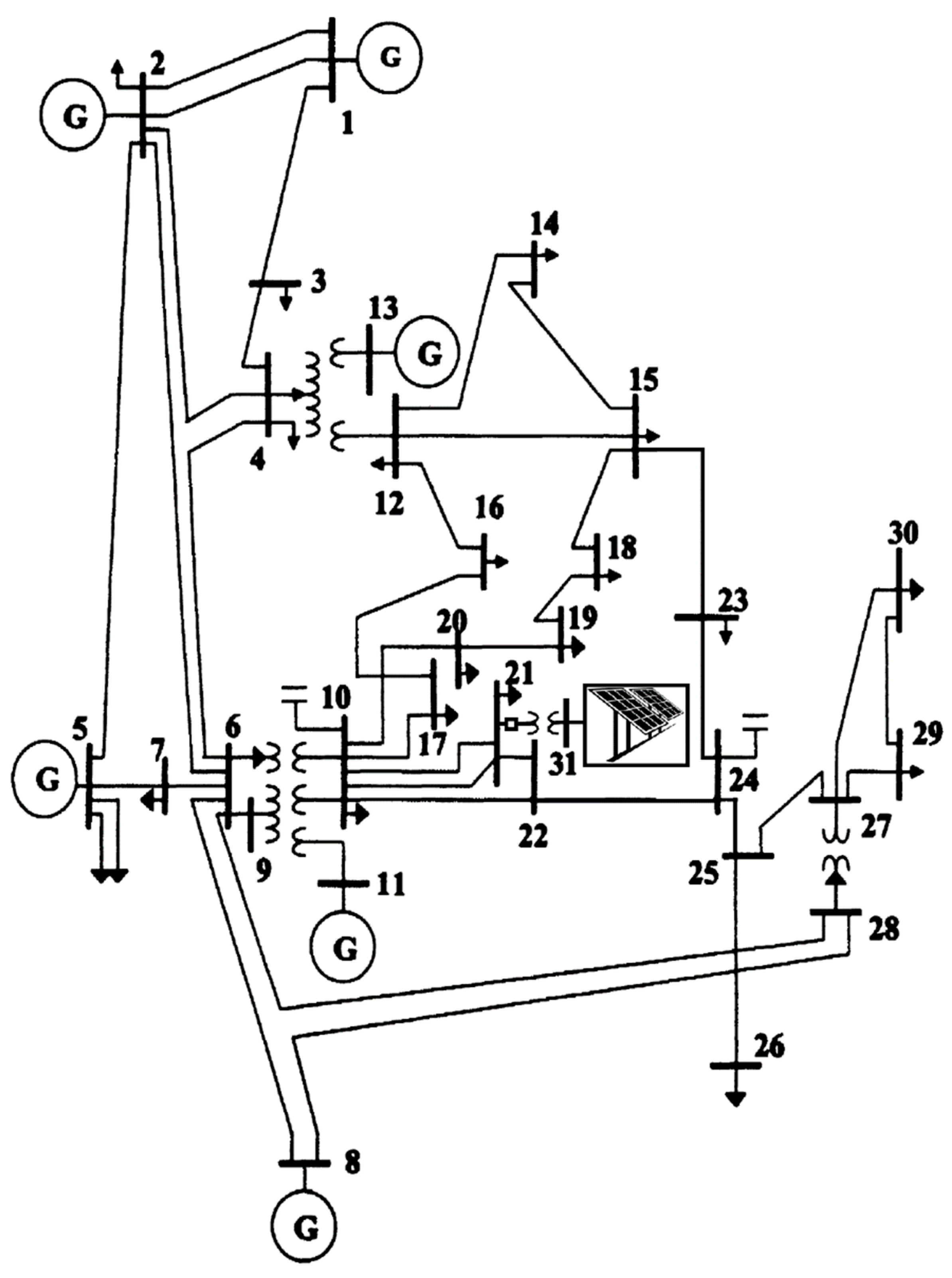
3.1. Case I: Base Case

It is basically the DSM techniques; neither CVR nor DLC was implemented. No distributed generator was added to the system.

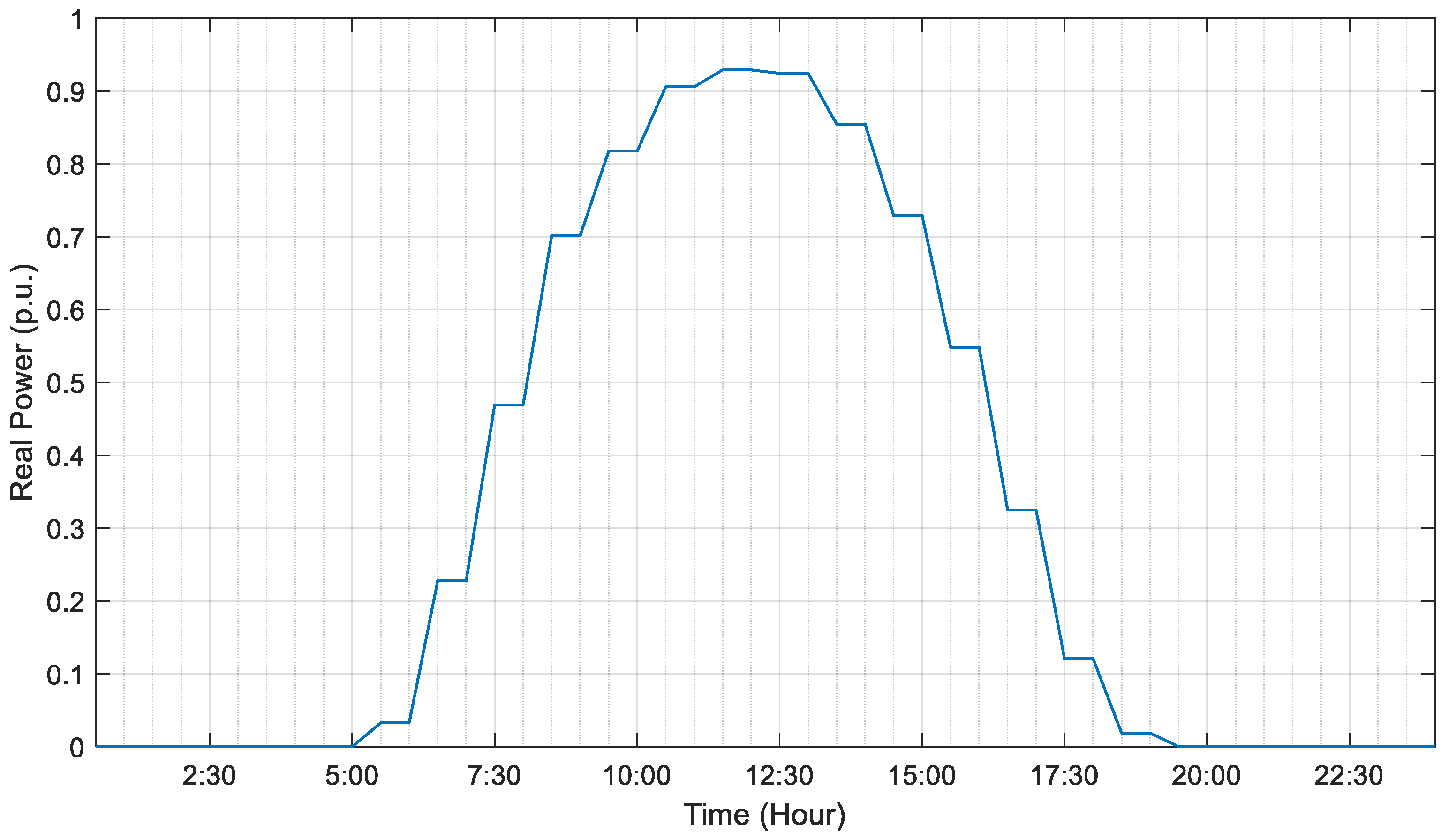
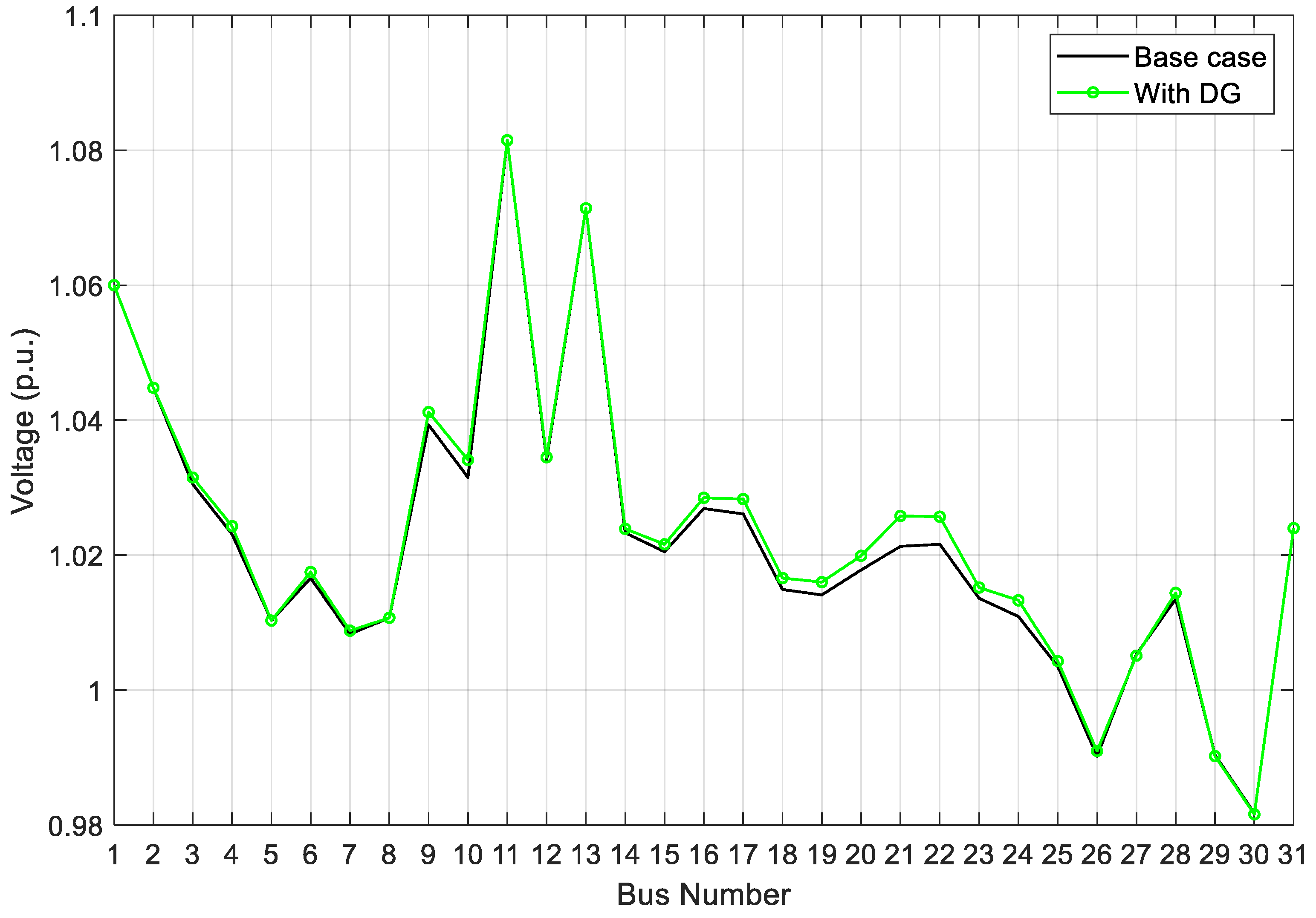
3.2. Case II: With DG, without CVR and DLC

Distributed generation technology has created an important role in smart grids due to its technical, environmental and economic benefits [2,3,4]. DG can improve reliability as well as provide some other technical benefits: reduced line losses, reactive power control, congestion mitigation at distribution and transmission level, increased system capacity, lower reserve margin requirements at low cost and shorter power outages [54].
In this case, the optimal location of the distributed generator was established based on minimizing power losses of the entire test system. The best location was found to be bus number 21 [2,54]. A Photovoltaic distributed generator was added to the determined bus location. The optimal capacity was found to be very large, namely 100 s MW, thus a smaller DG capacity was chosen to simulate a more realistic case [2,54]. The capacity chosen was 10.233 MW. Figure 6 illustrates the output power of the PV system used in the grid-connected test system. It is worth mentioning that the output power of a PV array is influenced by solar irradiance. It is obvious that the output power of PV modules increases when the irradiance increases, and hence the capacity of PV will slightly increase [5].
Figure 7 shows the voltage profile for the test system before and after the DG interconnection. It is observed that voltage the profile slightly increased; this small variation is due to the use of small capacity of PV compared to total system capacity. However, this integration of PV may alleviate voltage violations when CVR is applied.

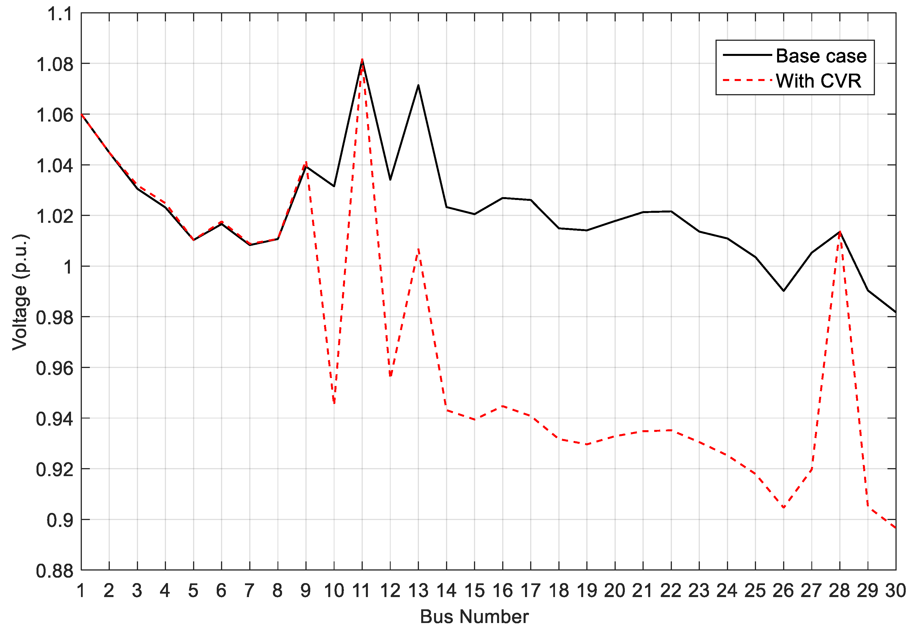
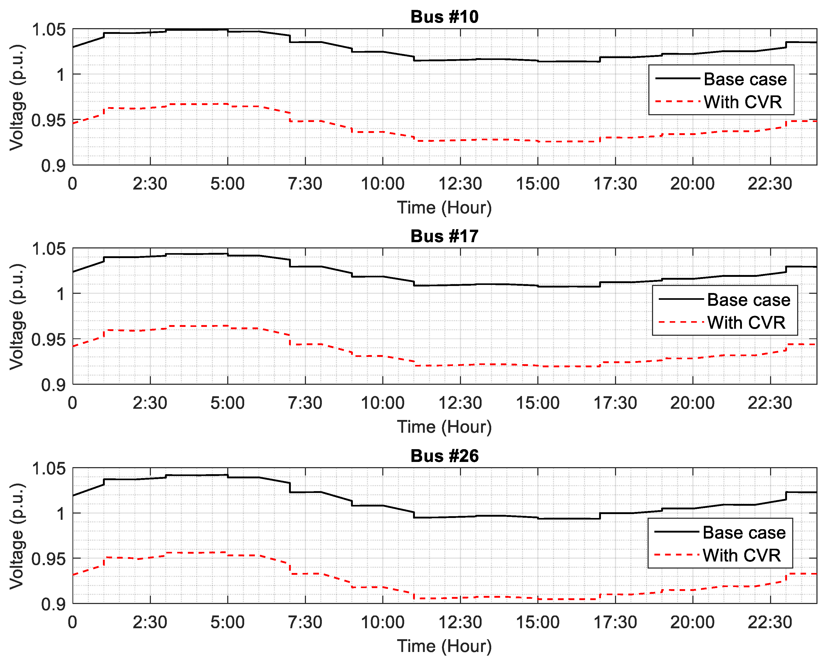
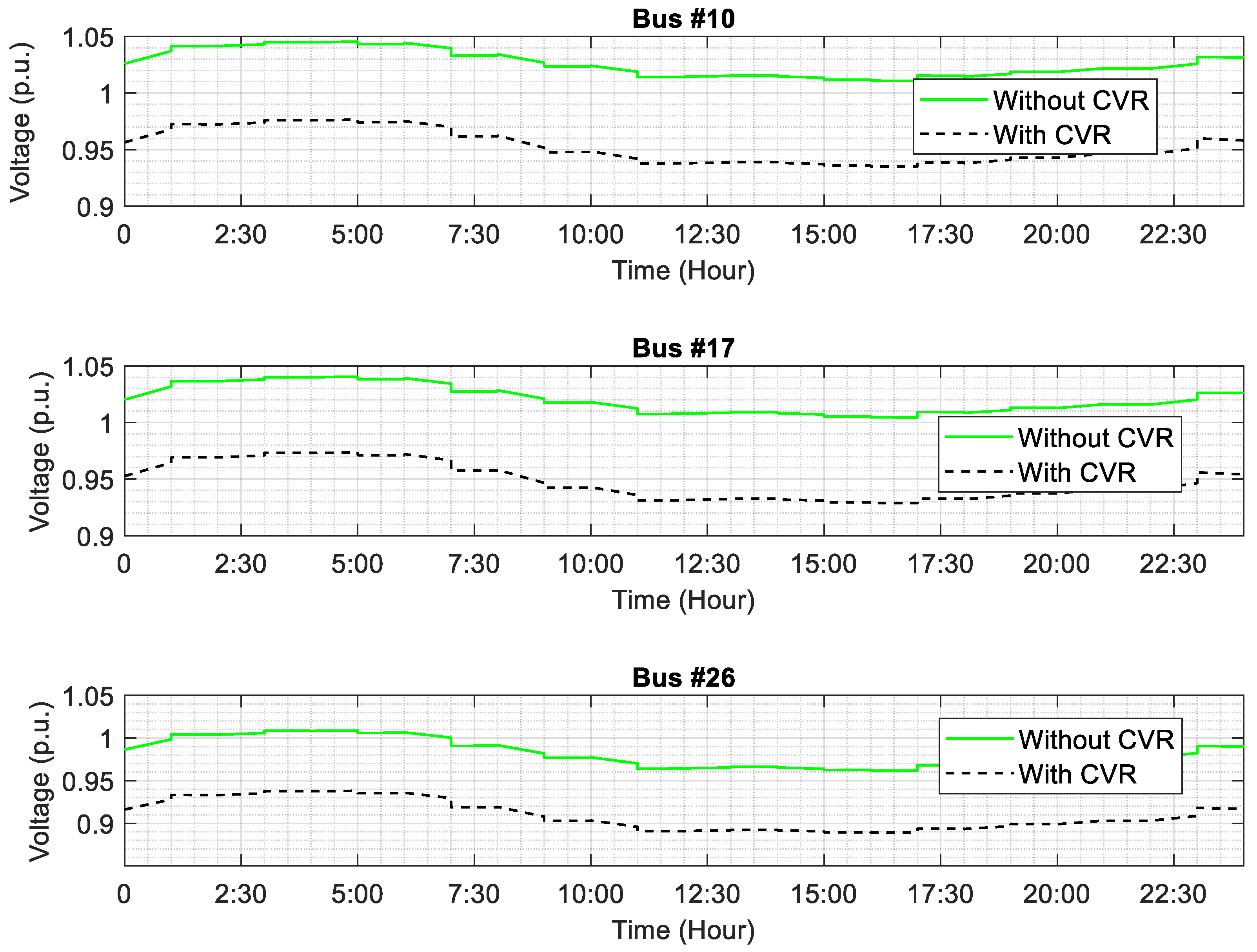
3.3. Case III: With CVR, without DG and DLC

The algorithm used starts by making all tap-changing transformers go to their default tap position (defined as 1.0 pu voltage), and it takes two set points Vmin and Vs. The algorithm measures the voltage at all loads in the 33-kV region every 30 min, and then it decides whether to increase, decrease or not change the tap position. If any load bus has a voltage lower than Vmin the tap position is increased; if any load bus has a voltage higher than Vs while all other load buses’ voltages are higher than Vmin, the tap position is decreased; and, if all load buses’ voltages are between Vmin and Vs no change will occur.
For the IEEE 30-Bus test system, Vs must be set to 1.08 or less p.u. If it is chosen higher than 1.08, the saved energy will drop significantly (the CVR algorithm will be rendered useless). When the taps of the tap-changing transformers are lowered, the voltages of the 33-kV region buses drop, but the voltage of bus 29 remains slightly higher than 1.08 for all relevant tap positions, which is why whatever Vs is chosen, bus 29 will ensure that the algorithm will lower the taps until the bus with the lowest voltage in the 33-kV region (bus 26) will be just above 0.9 p.u. The Vs threshold will be entirely different for different test systems.
One can see the voltage profile of the 30-Bus IEEE system in Figure 8. The buses of interest here are the following buses found in the 33-kV region: 10, 12, 14, 15, 16, 17, 18, 19, 20, 21, 23, 24, 26, 29 and 30. The aforementioned buses’ voltages can be seen to drop after the algorithm is implemented. In addition, as a result of voltage reduction, the active and reactive powers have dramatically reduced, as presented in Table 2 and Table 3.
The fact that the CVR reduced 3% of the real power consumed by most loads in the 33-kV region is a testimony of how effective this technique is. The voltage reduction done should affect no customer negatively since they are getting an appropriate value of voltage (more than 0.9 pu), and they are getting constant power. The algorithm used is a closed loop control algorithm, which means that, not matter what load shape or massive load changes have happened, this algorithm can detect them (every 30 min) and try to adapt (sometimes a little bit slowly). The CVR algorithm managed to decrease consumed power, reduce system losses and provide the system with a voltage control scheme to automatically manage rapid voltage changes.
In Figure 9, one can see the voltages on buses 10, 17 and 26 along the 24-h simulation with a varying load shape. The voltages were reduced to a very good extent while remaining above the Vs a considerable amount of time, which is still fine since this will be nearly impossible to overcome when dealing with a lot of loads that have different voltages. The important notion is that all the load buses’ voltages remained above Vmin.

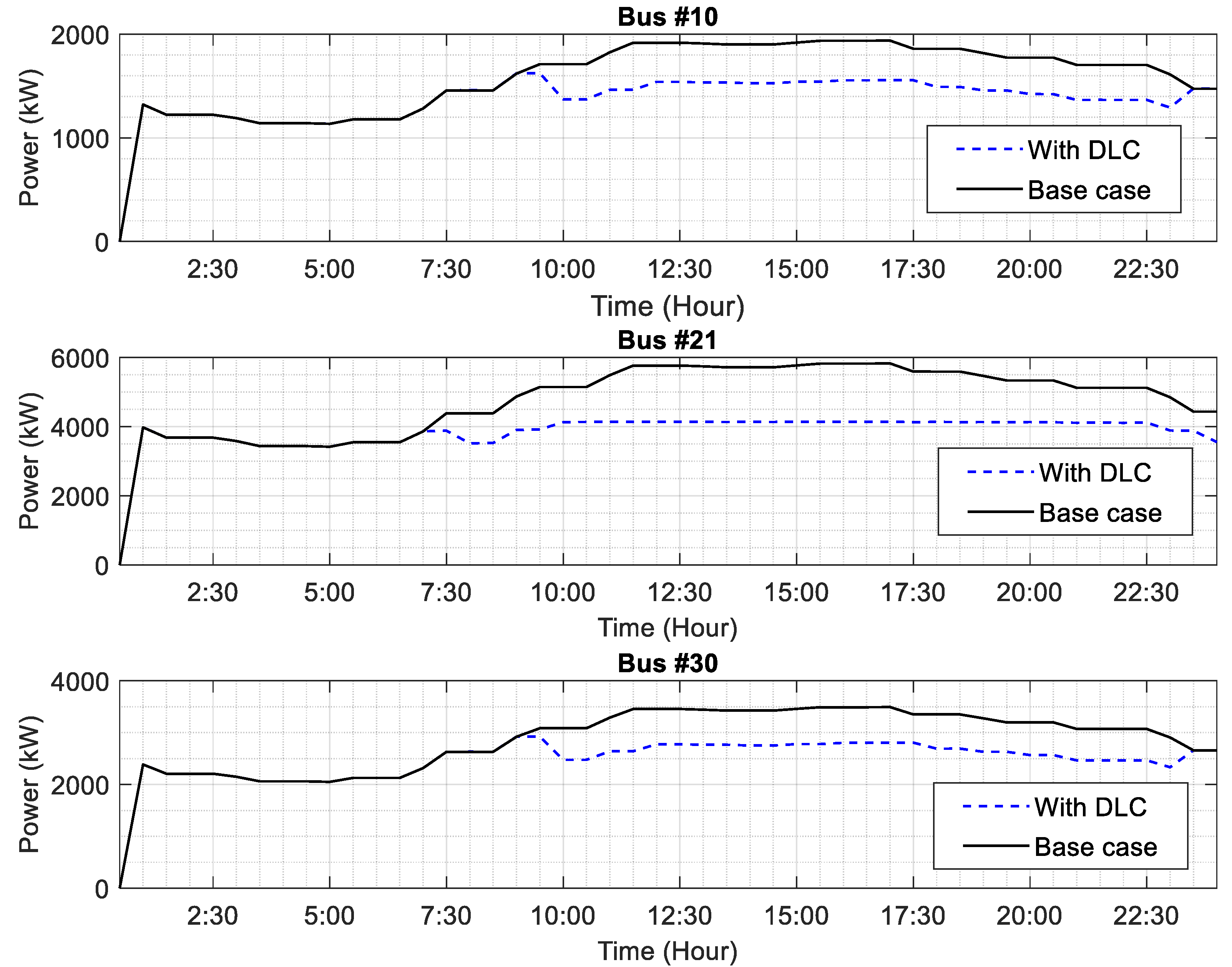
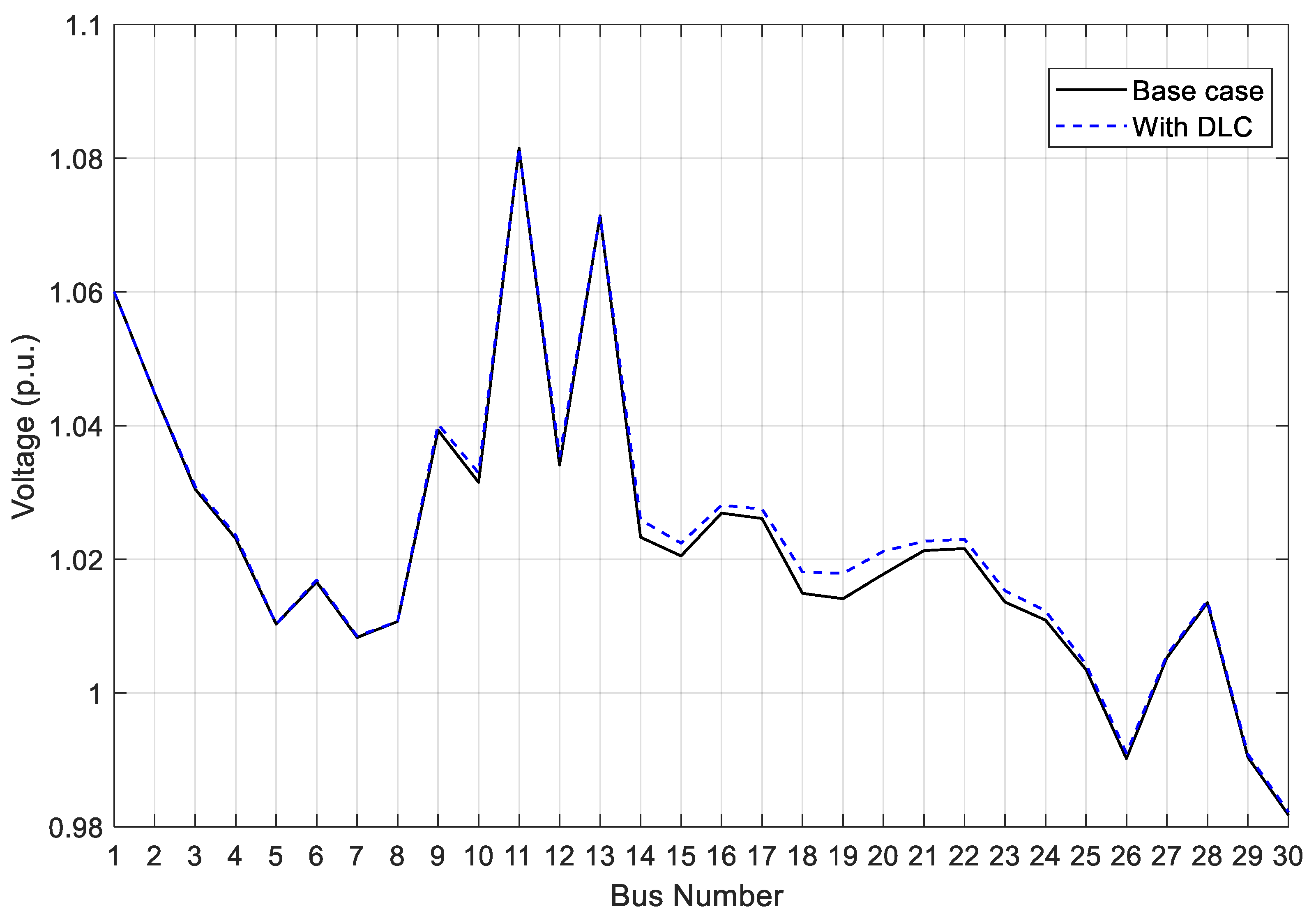
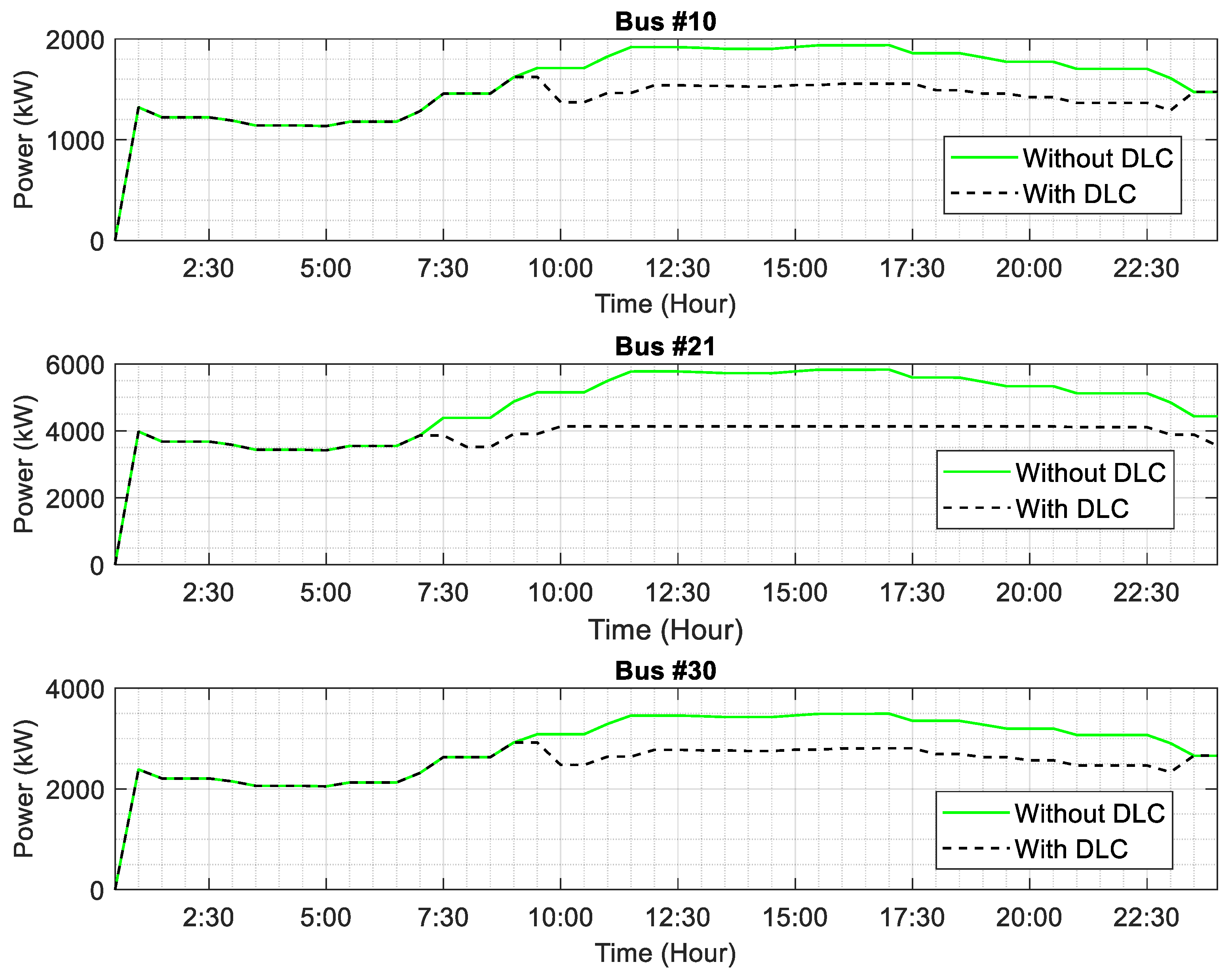
3.4. Case IV: With DLC, without DG and CVR

Mainly, the algorithm measures the power of each group over 24-h period. It starts by comparing each load with its pre-declared threshold (PTH) during an interval of 30 min. Once the consumed power by the loads/users exceeds this threshold, load control is taken. DLC curtails 10–30% of the load, maintaining the loads with the highest priority active. Finally, if consumption drops below PTH, the algorithm automatically connects the curtailed percentage back to the load.
In Figure 10, one can see the power of loads 10, 21 and 30 along the 24-h simulation with a varying load shape. According to Table 4, the consumed power of each load was considerably reduced when exceeding its tie-line threshold, as several loads were curtailed according to the aforementioned algorithm. In Figure 11, a small increase in voltage is observed as 10–30% of consumed load is curtailed, as if the load has become lightly loaded. As a general result, the advantages of this algorithm are lowered system losses and lowered consumed power.

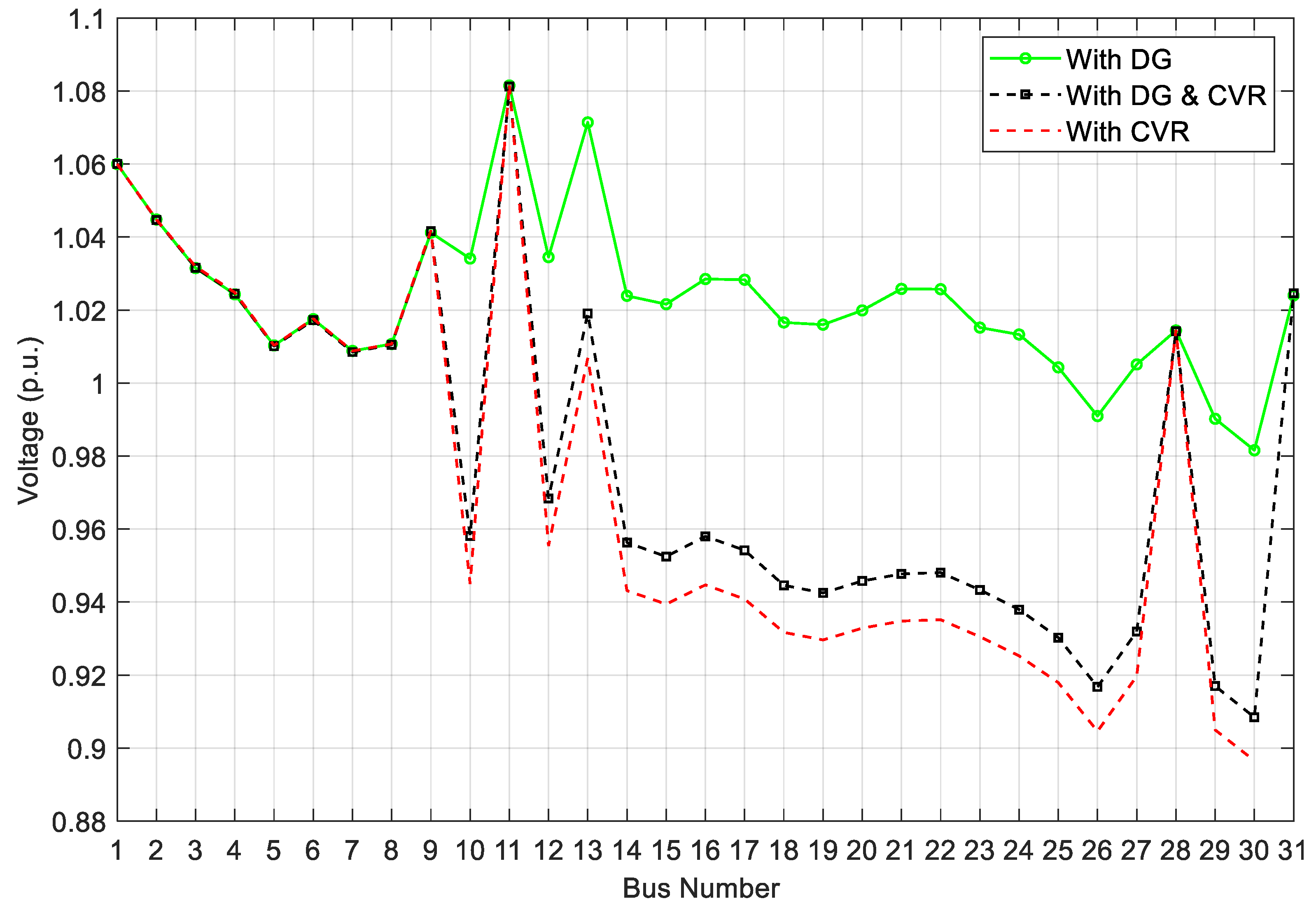
3.5. Case V: With CVR and DG, without DLC

In this case, the same CVR algorithm was used as in Case III. This case was simulated to test the effect of adding a PV system at the optimal location (Bus 21) on the CVR technique. Figure 12 shows the voltage profiles for the test system with/without PV in the presence of CVR. They have similar profiles, but the magnitude varies from bus to bus; it is clear that the voltage profile in the presence of DG and CVR is slightly higher in magnitude compared to the voltage profile in the presence of CVR technique alone. Under some circumstances, the integration of PV may alleviate voltage violations when CVR is applied.
Table 5 and Table 6 present the active and reactive power with/without CVR in the presence of DG. By comparing the tables for Case V with the tables for Case III, one can see that the effect the DG has on the CVR is a non-positive one. The DG decreased the saved active and reactive powers. On the other hand, the active and reactive powers consumed by the loads in the presence of the DG are slightly less. Thus, the overall effect of the DG is non-positive, but it is not that influential. The pros and cons of this case are similar to those of Case III alongside more technical, environmental and economic benefits at the system level due to the integration of the PV unit.
The voltages on buses 10, 17 and 26 along the 24-h simulation with a varying load shape with/without CVR in the presence of DG are shown in Figure 13. The presence of small PV unit did not provide significant difference compared to the case of implementing CVR algorithm alone.

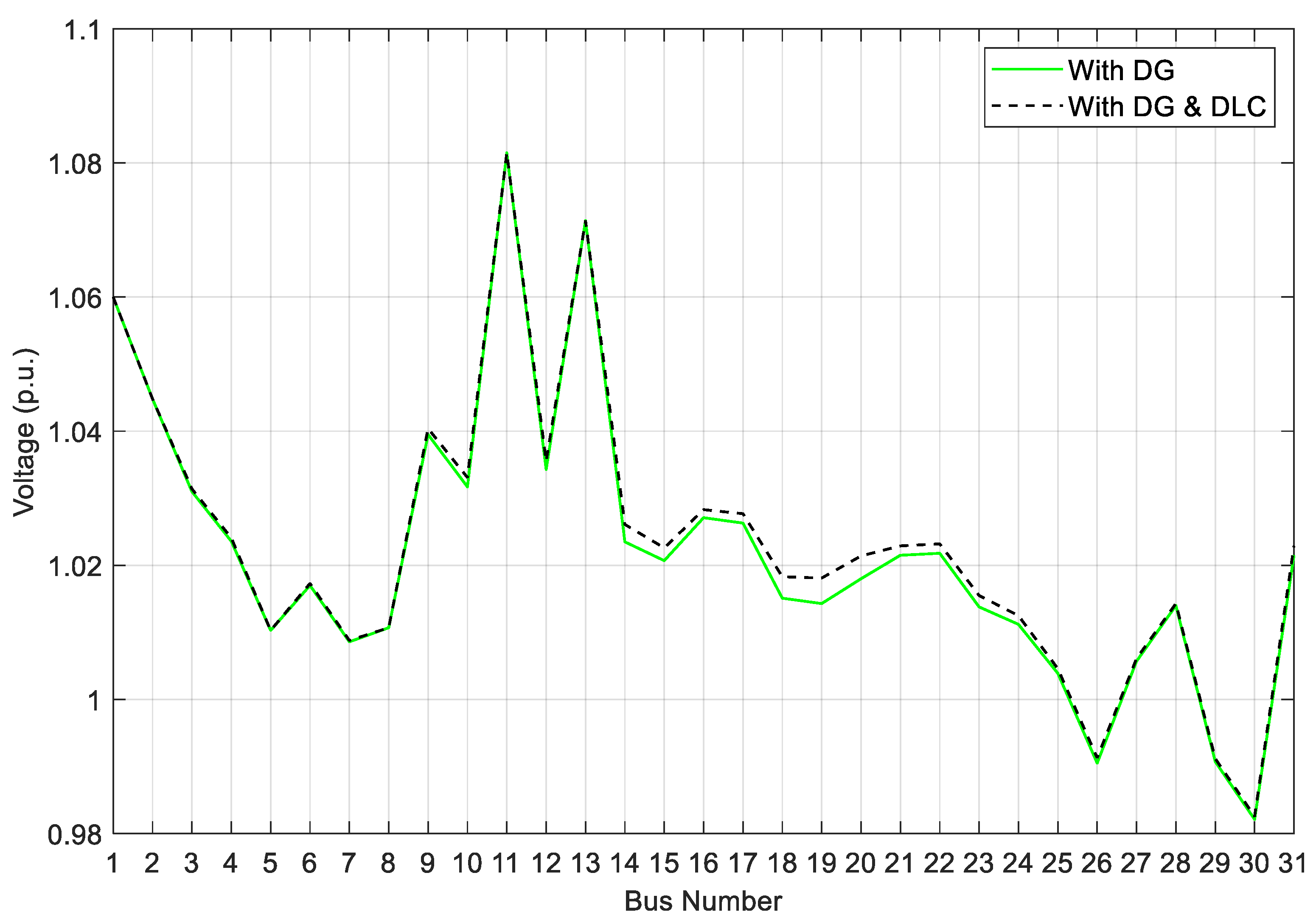
3.6. Case VI: With DLC and DG, without CVR

In this case, the same DLC algorithm was used as in Case IV. This case was simulated to test the effect of adding a PV system on the DLC technique. Figure 14 and Figure 15 show the power vs. time and the voltage profiles, respectively, for the test system with/without PV in the presence of DLC. It is observed that the real power and voltage in the presence of PV unit did not provide significant difference compared to the case of implementing DLC algorithm alone.
The active power and active power reduction with/without DLC in the presence of DG are evaluated for the concerned buses; the results are summarized in Table 7. As in Case V, the effect the DG had on the DSM technique (DLC) is a slightly non-positive one. The DG lowered the saved powers, but it also lowered the consumed powers. Thus, it can be seen as a neutral effect, unless the penetration level of the DG is extremely high. The pros and cons of this case are similar to those of Case IV alongside the other benefits mentioned above due to the interconnection of the PV.

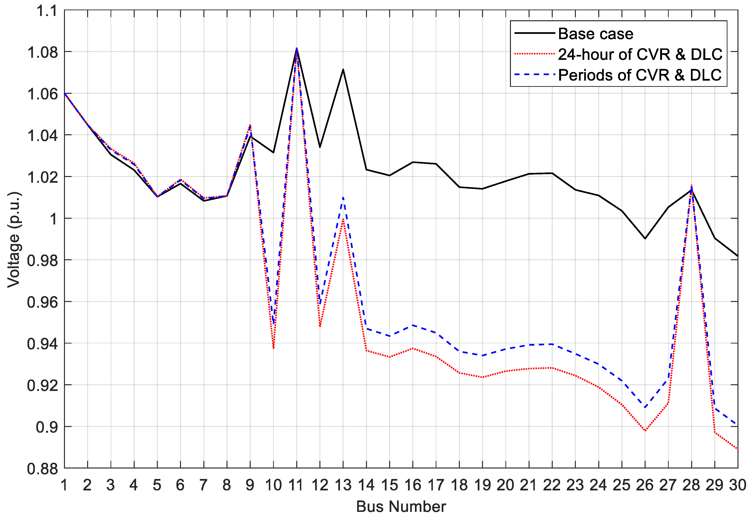
3.7. Case VII: With CVR and DLC, without DG

The combination of CVR and DLC was tested based on the two methods mentioned above. Figure 16 illustrates the variation of power and Figure 17 demonstrates the voltage profile; these figures include the base case and the aforementioned methods. The results obtained for this case regarding the active and reactive power are summarized in Table 8 and Table 9. The advantages of this scenario are the reduced system losses, reduced consumed power and the increased voltage control capability; thus, any voltage variation caused by DLC can be rectified by the CVR algorithm. Obviously, the dominant result was established by the implementation of the first method, where DLC and CVR are running through the entire 24 h. DLC forms the major impact on power reduction compared to CVR. As the power decreases, the voltage decreases, hence CVR does not take part in curtailing power at some points. Thus, the 24-h scheme has much better results.

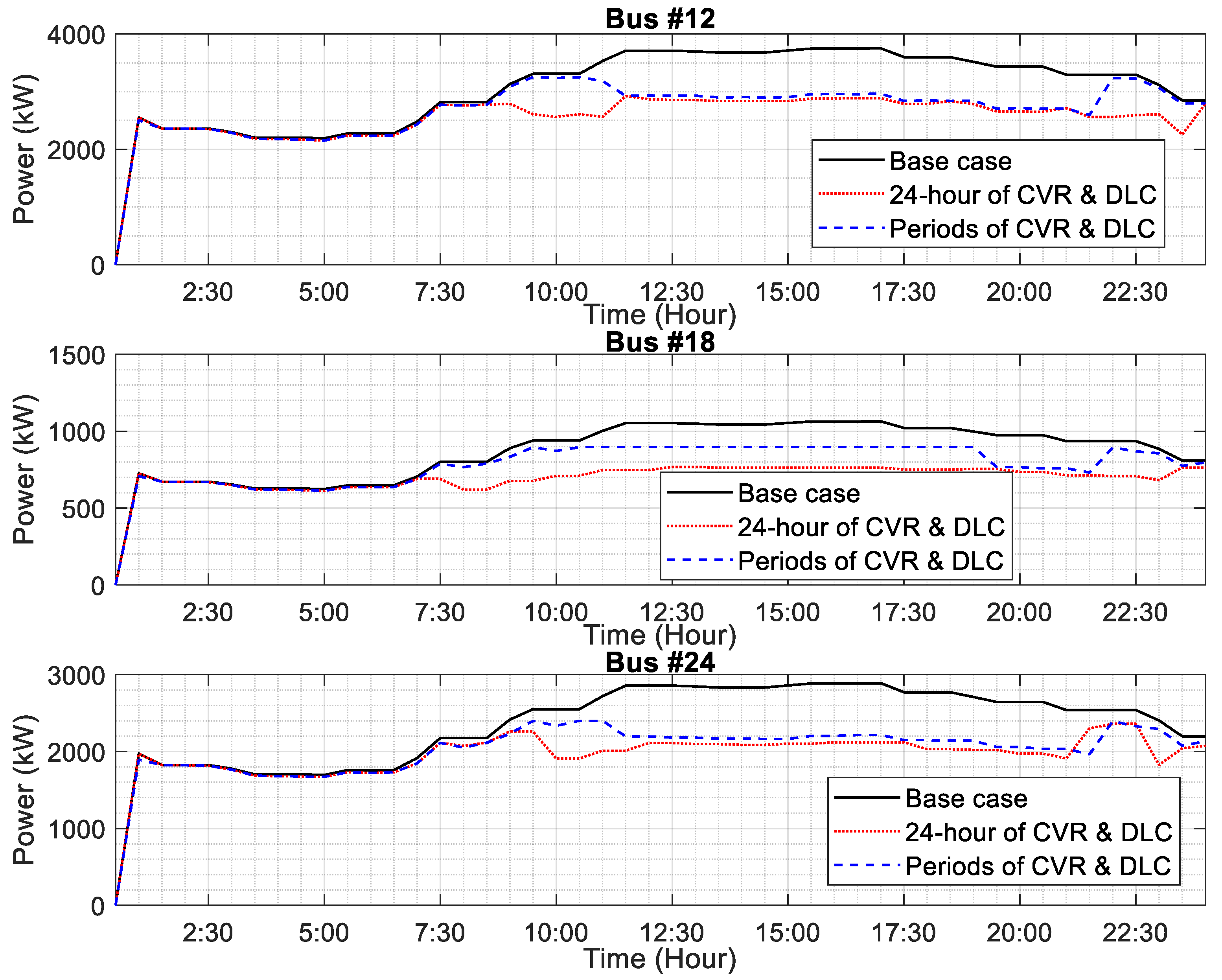
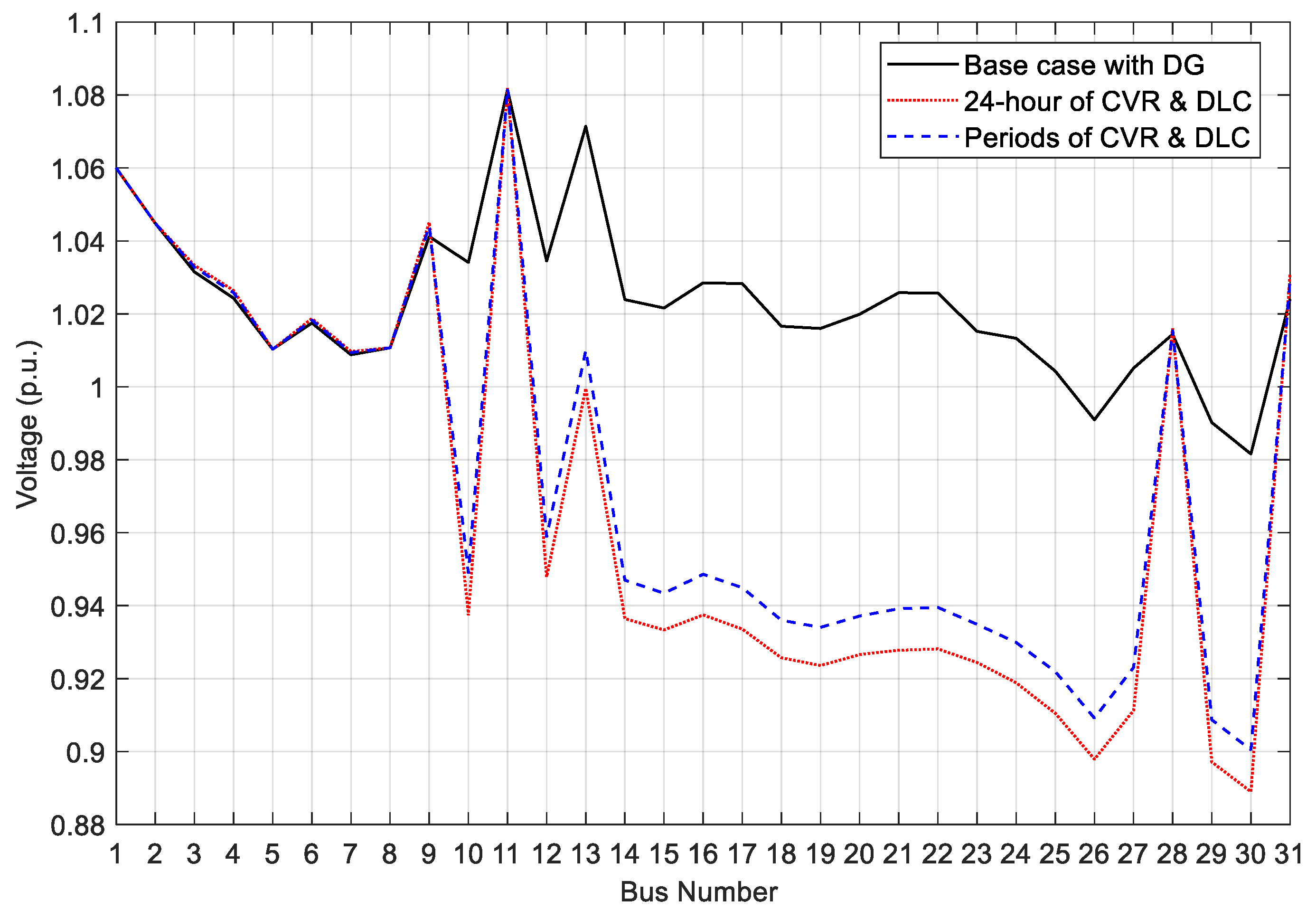
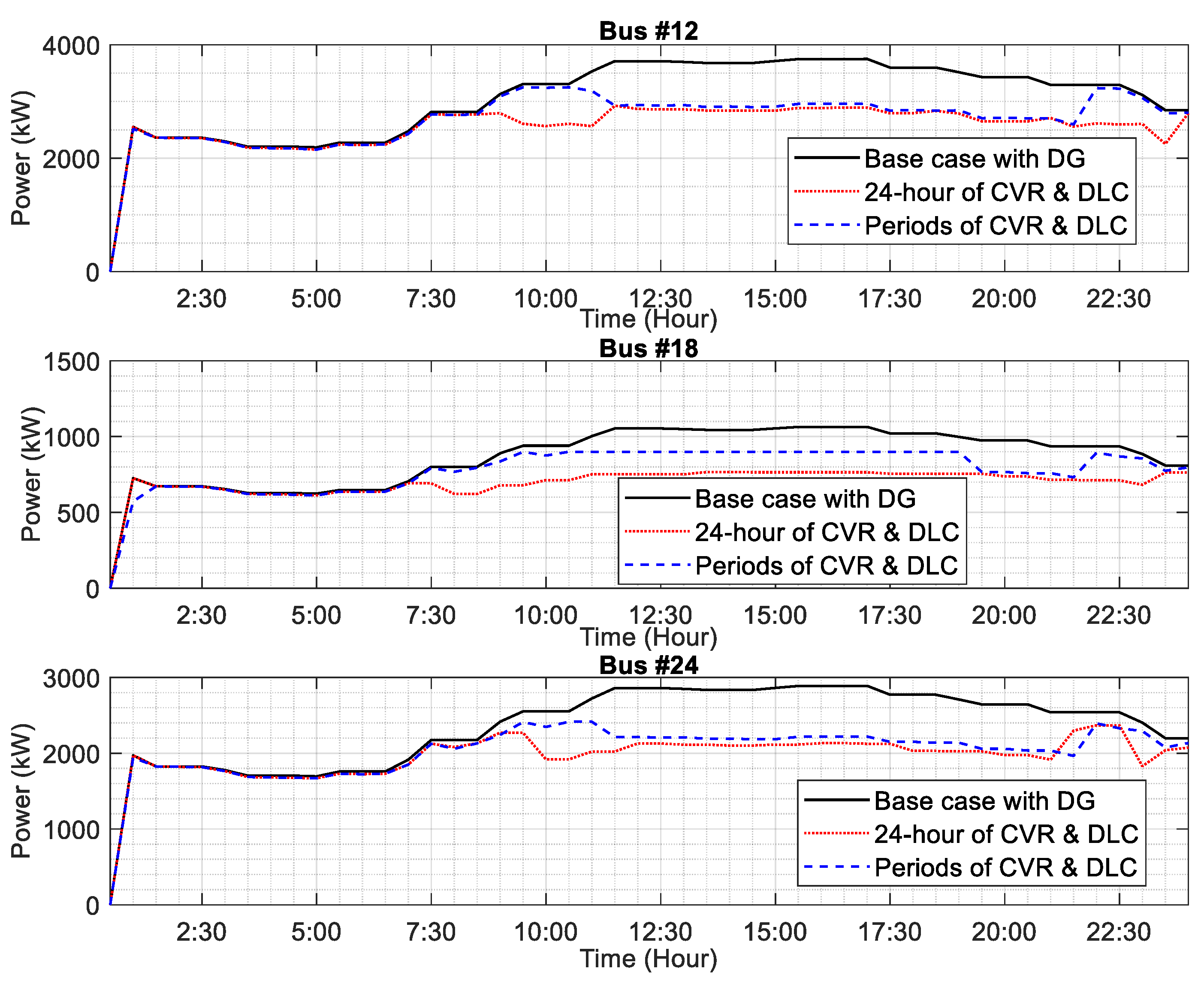
3.8. Case VIII: With DG, CVR and DLC

Case VIII is similar to the previous one, but the impact of photovoltaic distributed generator is considered. The aforementioned methods (24-h and periods) were used to verify the proposed algorithms. Figure 18 and Figure 19 show the voltage profiles and power vs. time, respectively, for the test system with CVR and DLC in the presence of PV. It is observed that the real power and voltage in the presence of PV did not provide significant difference compared to the case of implementing algorithms without PV.
Table 10 and Table 11 show the results for this case. By comparing these tables with the tables for previous case, one can see that the effect the DG has on the CVR and DLC is a slightly negative one. The DG decreased the saved active and reactive powers. However, the active and reactive powers consumed by the loads in the presence of the DG are slightly less. Thus, the Overall effect of the DG is non-positive but it is not that influential. The pros and cons of this case are similar to those of Case VII alongside more technical, environmental and economic benefits due to the integration of the DG. From the irradiance perspective, the comparison between a summer day of good irradiance and a cold day of zero irradiance (in worst case) can be related to Cases VIII and VII, respectively. As indicated above, the PV integration causes minor negative effects on DSM techniques; if Case VII were presumed to be the zero irradiance of Case VIII in certain weather conditions, the variation in irradiance would have very small effect in terms of voltage profile and saved energy.

3.9. Comparison

The consumed and saved energies along with the energy losses of all considered cases are compared in this section; the results are summarized in Table 12.
By comparing the saved, consumed and lost energies of all eight cases one can see that Case VII (24-h technique) yields the best results with the lowest network losses and the highest saved energy. One can examine all the DSM cases and realize that the DLC technique lowered the losses in the network as well as saved energy when compared to Case I or II. DLC can save much more energy than CVR, since CVR is constrained by voltage standards. DLC reduces energy losses since it decreases the power of the loads, which will lower the current drawn from the source, thus reducing losses. When deploying DLC and CVR together, CVR can control any voltage change caused by DLC when the load powers are varied. The effect of the DG on bus 21 is minimal, but it is important to notice that it affects CVR losses more severely than DLC losses. Thus, in summary, CVR can decrease consumed energy and increase the system’s voltage control capabilities. DLC lowered circuit losses and consumed energy by a larger margin than CVR. The combined algorithm reduced system losses and consumed energy and gave the system increased voltage control capabilities.

4. Conclusions

The individual performances of the DLC and CVR techniques were confirmed, regarding reduction in energy losses and reduction in consumed energy; as a result, nearly 5% and 4.3% of saved energy is achieved when applying DLC and CVR, respectively. The implementation of CVR concurrently with DLC yields in the best results with the lowest network losses and the highest of approximately 9.3% of the saved energy. The commutations between CVR and DLC occurred among different consumption periods where generally DLC is efficient to operate in high power consumption periods while CVR gives better controllability and voltage reduction when the consumption is minimal and this scenario yields in nearly 6% of energy saved. Moreover, the 24-h algorithm yields the best outcome as it is adaptive to choosing the appropriate DSM techniques when applicable. On the other hand, the periods algorithm is limited to operate only one DSM technique during the predefined interval, which prevents the presence of the other. Finally, the PV integration provides an improvement in terms of voltage profile and this integration of PV may alleviate voltage violations with CVR implementation. However, PV integration causes minor negative effects on DSM techniques, thus they can be neglected since this integration provides a wide range of mutual benefits to the customer, the utility and the market.

Author Contributions

All authors contributed extensively to the work presented in this paper. J.A.S. proposed the topic, conceived the solution and supervised the whole work. Z.W., F.A. and J.D. studied and programed the algorithms. S.F. and G.Z. contributed materials and reviewed the results. All authors have read and agreed to the published version of the manuscript.

Funding

This research received no external funding.

Acknowledgments

The present work was realized in the framework of the Research Cooperation Agreement between the Engineering Department of the University of Palermo and the Department of Electrical and Computer Engineering of Birzeit University, for the project DGWG (Distributed Generation integration in Weak Grids).

Conflicts of Interest

The authors declare no conflict of interest.

References

  1. Sa’ed, J.A.; Favuzza, S.; Massaro, F.; Musca, R.; Zizzo, G.; Cagnano, A.; De Tuglie, E. Effects of Demand Side Management on the Operation of an Isolated LV Microgrids. In Proceedings of the IEEE/EEEIC 2019, Genova, Italy, 11–14 June 2019; pp. 1–6. [Google Scholar]
  2. Sa’ed, J.A.; Amer, M.; Bodair, A.; Baransi, A.; Favuzza, S.; Zizzo, G. Effect of integrating photovoltaic systems on electrical network losses considering load variation. In Proceedings of the IEEE/EEEIC 2018, Palermo, Italy, 12–15 June 2018; pp. 1–6. [Google Scholar]
  3. Sa’ed, J.A.; Awad, A.; Favuzza, S.; Massaro, F.; Zizzo, G. A Framework to Determine Maximum Capacity of Interconnecting DGs in Distribution Networks. In Proceedings of the IEEE/CPE-POWERENG 2018, Doha, Qatar, 10–12 April 2018; pp. 1–6. [Google Scholar]
  4. Sa’ed, J.A.; Jubran, M.K.; Favuzza, S.; Ippolito, M.G.; Massaro, F. Reassessment of voltage stability for distribution networks in presence of DG. In Proceedings of the IEEE/EEEIC 2016, Florence, Italy, 7–10 June 2016; pp. 1–5. [Google Scholar]
  5. Motan, N.; Abu-Khaizaran, M.; Quraan, M. Photovoltaic Array Modelling and Boost-Converter Controller-Design for a 6kW Grid Connected Photovoltaic System—DC Stage. In Proceedings of the IEEE/EEEIC 2018, Palermo, Italy, 12–15 June 2018; pp. 1–6. [Google Scholar]
  6. Sa’ed, J.A.; Favuzza, S.; Ippolito, M.G.; Massaro, F. Integration Issues of Distributed Generators Considering Faults in Electrical Distribution Networks. In Proceedings of the IEEE/Energy Conference 2014, Cavtat, Croatia, 13–16 May 2014; pp. 1062–1068. [Google Scholar]
  7. Sa’ed, J.A.; Favuzza, S.; Ippolito, M.G.; Massaro, F. An Investigation of Protection Devices Coordination Effects on Distributed Generators Capacity in Radial Distribution Systems. In Proceedings of the IEEE/ICCEP 2013, Alghero, Italy, 11–13 June 2013; pp. 686–692. [Google Scholar]
  8. Madani, V.; Das, R.; Aminifar, F.; McDonald, J.; Venkata, S.S.; Novosel, D.; Bose, A.; Shahidehpour, M. Distribution Automation Strategies Challenges and Opportunities in a Changing Landscape. IEEE Trans. Smart Grid 2015, 6, 2157–2165. [Google Scholar] [CrossRef]
  9. Favuzza, S.; Galioto, G.; Ippolito, M.; Massaro, F.; Milazzo, F.; Pecoraro, G.; Sanseverino, E.R.; Telaretti, E. Real-time pricing for aggregates energy resources in the Italian energy market. Energy 2015, 87, 251–258. [Google Scholar] [CrossRef]
  10. Meyabadi, A.F.; Deihimi, M. A review of demand-side management: Reconsidering theoretical framework. Renew. Sustain. Energy Rev. 2017, 80, 367–379. [Google Scholar] [CrossRef]
  11. Sarker, E.; Halder, P.; Seyedmahmoudian, M.; Jamei, E.; Horan, B.; Mekhilef, S.; Stojcevski, A. Progress on the demand side management in smart grid and optimization approaches. Int. J. Energy Res. 2020, 1–29. [Google Scholar] [CrossRef]
  12. Lu, X.; Zhou, K.; Zhang, X.; Yang, S. A systematic review of supply and demand side optimal load scheduling in a smart grid environment. J. Clean. Prod. 2018, 203, 757–768. [Google Scholar] [CrossRef]
  13. Silva, B.N.; Khan, M.; Han, K. Futuristic Sustainable Energy Management in Smart Environments: A Review of Peak Load Shaving and Demand Response Strategies, Challenges, and Opportunities. Sustainability 2020, 12, 5561. [Google Scholar] [CrossRef]
  14. Jabir, H.J.; Teh, J.; Ishak, D.; Abunima, H. Impacts of Demand-Side Management on Electrical Power Systems: A Review. Energies 2018, 11, 1050. [Google Scholar] [CrossRef] [Green Version]
  15. Logenthiran, T.; Srinivasan, D.; Shun, T.Z. Demand Side Management in Smart Grid Using Heuristic Optimization. IEEE Trans. Smart Grid 2012, 3, 1244–1252. [Google Scholar] [CrossRef]
  16. Yang, P.; Chavali, P.; Gilboa, E.; Nehorai, A. Parallel Load Schedule Optimization with Renewable Distributed Generators in Smart Grids. IEEE Trans. Smart Grid 2013, 4, 1431–1441. [Google Scholar] [CrossRef]
  17. Wu, Z.; Tazvinga, H.; Xia, X. Demand side management of photovoltaic-battery hybrid system. Appl. Energy 2015, 148, 294–304. [Google Scholar] [CrossRef] [Green Version]
  18. Palma-Behnke, R.; Benavides, C.; Aranda, E.; Llanos, J.; Sáez, D. Energy management system for a renewable based microgrid with a demand side management mechanism. In Proceedings of the IEEE Symposium on Computational Intelligence Applications in Smart Grid 2011, Paris, France, 11–15 April 2011; pp. 1–8. [Google Scholar]
  19. Fan, W.; Liu, N.; Zhang, J. An Event-Triggered Online Energy Management Algorithm of Smart Home: Lyapunov Optimization Approach. Energies 2016, 9, 381. [Google Scholar] [CrossRef] [Green Version]
  20. Solanki, B.V.; Raghurajan, A.; Bhattacharya, K.; Canizares, C.A. Including smart loads for optimal demand response in integrated energy management systems for isolated microgrids. IEEE Trans. Smart Grid. 2017, 8, 1739–1748. [Google Scholar] [CrossRef]
  21. Nguyen, H.K.; Bin, S.J.; Han, Z. Distributed Demand Side Management with Energy Storage in Smart Grid. IEEE Trans. Parallel Distrib. Syst. 2015, 26, 3346–3357. [Google Scholar] [CrossRef]
  22. Amrollahi, M.H.; Bathaee, S.M.T. Techno-economic optimization of hybrid photovoltaic/wind generation together with energy storage system in a stand-alone micro-grid subjected to demand response. Appl. Energy 2017, 202, 66–77. [Google Scholar] [CrossRef]
  23. Mohsenian-Rad, A.-H.; Wong, V.W.S.; Jatskevich, J.; Schober, R.; Leon-Garcia, A. Autonomous Demand-Side Management Based on Game-Theoretic Energy Consumption Scheduling for the Future Smart Grid. IEEE Trans. Smart Grid 2010, 1, 320–331. [Google Scholar] [CrossRef] [Green Version]
  24. Bharathi, C.; Rekha, D.; Vijayakumar, V. Genetic Algorithm Based Demand Side Management for Smart Grid. Wirel. Pers. Commun. 2017, 93, 481–502. [Google Scholar] [CrossRef]
  25. Macedo, M.N.Q.; Galo, J.J.M.; de Almeida, L.A.L.; Lima, A.D.C. Demand side management using artificial neural networks in a smart grid environment. Renew. Sustain. Energy Rev. 2015, 41, 128–133. [Google Scholar] [CrossRef]
  26. Mahmood, A.; Ullah, M.N.; Razzaq, S.; Basit, A.; Mustafa, U.; Naeem, M.; Javaid, N. A New Scheme for Demand Side Management in Future Smart Grid Networks. Procedia Comput. Sci. 2014, 32, 477–484. [Google Scholar] [CrossRef] [Green Version]
  27. López, M.A.; de la Torre, S.; Martín, S.; Aguado, J.A. Demand-side management in smart grid operation considering electric vehicles load shifting and vehicle-to-grid support. Int. J. Electr. Power Energy Syst. 2015, 64, 689–698. [Google Scholar] [CrossRef]
  28. Samadi, P.; Mohsenian-Rad, H.; Schober, R.; Wong, V.W.S. Advanced Demand Side Management for the Future Smart Grid Using Mechanism Design. IEEE Trans. Smart Grid 2012, 3, 1170–1180. [Google Scholar] [CrossRef]
  29. Zhu, Z.; Tang, J.; Lambotharan, S.; Chin, W.H.; Fan, Z. An Integer Linear Programming Based Optimization for Home Demand-side Management in Smart Grid. In Proceedings of the IEEE PES conference on Innovative Smart Grid Technologies, Washington, DC, USA, 16–20 January 2012; pp. 1–5. [Google Scholar]
  30. Mohsenian-Rad, A.; Wong, V.W.S.; Jatskevich, J.; Schober, R. Optimal and autonomous incentive-based energy consumption scheduling algorithm for smart grid. In Proceedings of the IEEE PES conference on Innovative Smart Grid Technologies, Gothenburg, Sweden, 19–21 January 2010; pp. 1–6. [Google Scholar]
  31. Klaić, Z.; Fekete, K.; Šljivac, D. Demand side load management in the distribution system with photovoltaic generation. Tech. Gazette. 2015, 22, 989–995. [Google Scholar]
  32. Monyeia, C.G.; Adewumia, A.O. Demand Side Management potentials for mitigating energy poverty in South Africa. Energy Policy 2017, 111, 298–311. [Google Scholar] [CrossRef] [Green Version]
  33. Bhattarai, B.P.; Bak-Jensen, B.; Mahat, P.; Pillai, J.R.; Maier, M. Hierarchical control architecture for demand response in smart grids. In Proceedings of the 2013 IEEE PES APPEEC, Kowloon, China, 8–11 December 2013; pp. 1–6. [Google Scholar]
  34. Beal, J.; Berliner, J.; Hunter, K. Fast precise distributed control for energy demand management. In Proceedings of the sixth IEEE international conference on self-adaptive and self-organizing systems, Lyon, France, 10–14 September 2012; pp. 187–192. [Google Scholar]
  35. Schneider, K.P.; Fuller, J.C.; Tuffner, F.K.; Singh, R. Evaluation of Conservation Voltage Reduction (CVR) on a National Level; Tech. Report; Pacific Northwest National Laboratory PNNL-19596: Richland, MO, USA, 2010.
  36. Lefebvre, S.; Gaba, G.; Ba, A.O.; Asber, D.; Ricard, A.; Perreault, C.; Chartrand, D. Measuring the efficiency of voltage reduction at Hydro-Qubec distribution. In Proceedings of the 2008 IEEE Power and Energy Society General Meeting—Conversion and Delivery of Electrical Energy in the 21st Century, Pittsburgh, PA, USA, 20–24 July 2008; pp. 1–7. [Google Scholar]
  37. Sandraz, J.P.A.; Macwan, R.; Diaz-Aguilo, M.; McClelland, J.; De Leon, F.; Czarkowski, D.; Comack, C. Energy and Economic Impacts of the Application of CVR in Heavily Meshed Secondary Distribution Networks. IEEE Trans. Power Deliv. 2014, 29, 1692–1700. [Google Scholar] [CrossRef]
  38. Wilson, T.L. Measurement and verifications of distribution voltage optimization results for the IEEE Power & Energy Society. In Proceedings of the IEEE PES General Meeting, Providence, RI, USA, 25–29 July 2010; pp. 1–9. [Google Scholar]
  39. Chen, P.-C.; Salcedo, R.; Zhu, Q.; De Leon, F.; Czarkowski, D.; Jiang, Z.-P.; Spitsa, V.; Zabar, Z.; Uosef, R.E. Analysis of Voltage Profile Problems Due to the Penetration of Distributed Generation in Low-Voltage Secondary Distribution Networks. IEEE Trans. Power Deliv. 2012, 27, 2020–2028. [Google Scholar] [CrossRef]
  40. Bag, B.; Thakur, T. A Utility Initiative based Method for Demand Side Management and Loss Reduction in a Radial Distribution Network Containing Voltage Regulated Loads. In Proceedings of the 2016 ICEPES, Bhopal, India, 14–16 December 2016; pp. 52–57. [Google Scholar]
  41. Diaz-Aguilo, M.; Sandraz, J.; Macwan, R.; De Leon, F.; Czarkowski, D.; Comack, C.; Wang, D. Field-Validated Load Model for the Analysis of CVR in Distribution Secondary Networks: Energy Conservation. IEEE Trans. Power Deliv. 2013, 28, 2428–2436. [Google Scholar] [CrossRef]
  42. Gellings, C.W.; Parmenter, K.E. Demand-Side Management. In Energy Management and Conservation Handbook; Kreith, F., Goswami, D.Y., Eds.; CRC Press: Boca Raton, FL, USA, 2008; pp. 1–20. [Google Scholar]
  43. Gellings, C.W. The Smart Grid: Enabling Energy Efficiency and Demand Response; The Fairmont Press: Lilburn, Georgia, 2009; pp. 138–141. [Google Scholar]
  44. Hu, Z.; Han, X.; Wen, Q. Integrated Resource Strategic Planning and Power Demand-Side Management; Springer: Berlin, Germany, 2013; pp. 63–133. [Google Scholar]
  45. Medina, J.; Muller, N.; Roytelman, I. Demand Response and Distribution Grid Operations: Opportunities and Challenges. IEEE Trans. Smart Grid 2010, 1, 193–198. [Google Scholar] [CrossRef]
  46. Palensky, P.; Dietrich, D. Demand Side Management: Demand Response, Intelligent Energy Systems, and Smart Loads. IEEE Trans. Ind. Inform. 2011, 7, 381–388. [Google Scholar] [CrossRef] [Green Version]
  47. Alagoz, B.B.; Kaygusuz, A. A user-mode distributed energy management architecture for smart grid applications. Energy 2012, 44, 167–177. [Google Scholar] [CrossRef]
  48. Aghaei, J.; Alizadeh, M.-I. Demand response in smart electricity grids equipped with renewable energy sources: A review. Renew. Sustain. Energy Rev. 2013, 18, 64–72. [Google Scholar] [CrossRef]
  49. ANSI C84. Electric Power Systems and Equipment Voltage Ratings; NEMA: Arlington, VA, USA, 2011. [Google Scholar]
  50. EN 50160. Voltage Characteristics of Electricity Supplied by Public Electricity Networks; CENELEC: Brussels, Belgium, 2010. [Google Scholar]
  51. IEEE Std 1250-2018. IEEE Guide for Identifying and Improving Voltage Quality in Power Systems; IEEE: New York, NY, USA, 2018. [Google Scholar]
  52. Christie, R. Power Systems Test Case Archive. Available online: http://labs.ece.uw.edu/pstca/ (accessed on 10 August 2020).
  53. Bokhari, A.; Alkan, A.; Dogan, R.; Diaz-Aguilo, M.; De Leon, F.; Czarkowski, D.; Zabar, Z.; Birenbaum, L.; Noel, A.; Uosef, R.E. Experimental Determination of the ZIP Coefficients for Modern Residential, Commercial, and Industrial Loads. IEEE Trans. Power Deliv. 2014, 29, 1372–1381. [Google Scholar] [CrossRef]
  54. Sa’Ed, J.A.; Amer, M.; Bodair, A.; Baransi, A.; Favuzza, S.; Zizzo, G. A Simplified Analytical Approach for Optimal Planning of Distributed Generation in Electrical Distribution Networks. Appl. Sci. 2019, 9, 5446. [Google Scholar] [CrossRef] [Green Version]
Figure 1. DSM techniques.
Applsci 10 07551 g001
Figure 2. CVR algorithm flowchart.
Applsci 10 07551 g002
Figure 3. DLC algorithm flowchart.
Applsci 10 07551 g003
Figure 4. Combined CVR and DLC algorithm flowchart.
Applsci 10 07551 g004
Figure 5. IEEE 30-Bus modified single line diagram.
Applsci 10 07551 g005
Figure 6. Output power of the interconnected PV.
Applsci 10 07551 g006
Figure 7. Case II: Voltage profile with/without DG.
Applsci 10 07551 g007
Figure 8. Case III: Comparison of the voltage profile without CVR (Base case) and with CVR.
Applsci 10 07551 g008
Figure 9. Case III: Voltage vs. time with/without CVR.
Applsci 10 07551 g009
Figure 10. Case IV: Real power vs. time with/without DLC.
Applsci 10 07551 g010
Figure 11. Case IV: Comparison of the voltage profile without DLC (Base case) and with DLC.
Applsci 10 07551 g011
Figure 12. Case V: Voltage profiles with/without CVR in the presence of DG.
Applsci 10 07551 g012
Figure 13. Case V: Voltage vs. time with/without CVR in the presence of DG.
Applsci 10 07551 g013
Figure 14. Case VI: Power vs. time with/without DLC in the presence of DG.
Applsci 10 07551 g014
Figure 15. Case VI: Voltage profile with/without DLC in the presence of DG.
Applsci 10 07551 g015
Figure 16. Case VII: Power vs. time with/without CVR and DLC.
Applsci 10 07551 g016
Figure 17. Case VII: Voltage profile with/without CVR and DLC.
Applsci 10 07551 g017
Figure 18. Case VIII: Voltage profile with/without CVR and DLC in the presence of DG.
Applsci 10 07551 g018
Figure 19. Case VIII: Power vs. time with/without CVR and DLC in the presence of DG.
Applsci 10 07551 g019
Table 1. Summary of some results of algorithms used in DSM.
ReferenceMethod/TechniqueOutcome
[15]Heuristic-based load shifting techniqueReduced of peak-to-average ratio and minimized the energy cost
[16]Parallel autonomous optimization scheme with DR frameworkReduced of peak-to-average ratio and minimized the energy cost
[17]DR program with model predictive control methodMinimized the electricity bill on the customer side
[18]DSM mechanism along with artificial neural networkMinimized the operation cost
[19]Load scheduling method based on online event-triggered energy management algorithmReduced the electricity bill as well as ensured the user comfort level
[20]DR schemeAchieved an optimal power generation and peak load dispatch
[21]Load scheduling with game theory algorithmReduced peak load as well as energy payment for the consumers
[22]DR method with mixed-integer linear programmingReduced perational cost and peak load
[23]Autonomous and distributed
DSM scheme
Reduced of peak-to-average ratio and minimized the energy cost
[24]Load shifting technique using genetic algorithm Reduced of peak-to-average ratio
Table 2. Case III: Active power with/without CVR.
Bus/Load (#)Active Power without CVR (kW)Active Power with CVR (kW)Active Power Reduction (kW)Reduction Percentage (%)
1016061556.349.73.09
B1231053042.362.72.02
B141713.31651.761.63.60
B152264.12169.294.94.19
B16968.08936.2931.793.28
B172488.32393.295.13.82
B18882.03834.0248.015.44
B192617.72467.3150.45.75
B20606.83575.3731.465.18
B214831.54600.9230.64.77
B23881.73832.4149.325.59
B242395.12241.4153.76.42
B26958.49865.5492.959.70
B29657.45596.3561.19.29
B3028972580.5316.510.93
Table 3. Case III: Reactive power with/without CVR.
Bus/Load (#)Reactive Power without CVR (kvar)Reactive Power with CVR (kvar)Reactive Power Reduction (kvar)Reduction Percentage (%)
B10576.19533.6442.557.38
B122179.32006173.37.95
B14453.79423.9529.846.58
B15704.23656.9147.326.72
B16514.20478.5535.656.93
B171651.41533.5117.97.14
B18250.1233.1516.956.78
B19942.5879.463.16.69
B20195.62182.0613.566.93
B213152.62930.5222.17.04
B23443.42414.528.926.52
B24184417191256.78
B26607.67566.4241.256.79
B29238.29222.9215.376.45
B30494.28460.4533.836.84
Table 4. Case IV: Active power with/without DLC.
Bus/Load (#)Active Power without DLC (kW)Active Power with DLC (kW)Active Power Reduction (kW)Reduction Percentage (%)
B101608.81399.820912.99
B1231102567.3542.717.45
B141716.41392324.418.90
B152268.11778.149021.60
B16969.8793.1176.718.22
B172492.82081.2411.616.51
B18883.5715.2168.319.05
B192622.42129.449318.80
B20607.9349.7258.242.47
B214840.03921.5918.518.98
B23883.2722.8160.418.16
B242399.32068.6330.713.78
B26960.1778.7181.418.89
B29658.6596.462.29.44
B3029022526.3375.712.95
Table 5. Case V: Active power with/without CVR in the presence of DG.
Bus/Load (#)Active Power without CVR (kW)Active Power with CVR (kW)Active Power Reduction (kW)Reduction Percentage (%)
B101575.261529.4545.812.91
B123045.202986.3758.841.93
B141680.331621.1159.223.52
B152220.572129.6490.924.09
B16949.52919.7929.733.13
B172440.702351.5689.143.65
B18865.09819.1245.965.31
B192567.252423.37143.885.60
B20595.21565.2030.015.04
B214740.294527.46212.834.49
B23864.75817.4647.295.47
B242348.582202.52146.076.22
B26938.99849.4889.519.53
B29644.03584.8559.189.19
B302836.902530.71306.1910.79
Table 6. Case V: Reactive power with/without CVR in the presence of DG.
Bus/Load (#)Reactive Power without CVR (kvar)Reactive Power with CVR (kvar)Reactive Power Reduction (kvar)Reduction Percentage (%)
B10565.87524.2741.607.35
B122140.271970.78169.487.92
B14445.01416.6428.376.38
B15690.87645.8445.036.52
B16504.66470.7133.956.73
B171621.381508.95112.436.93
B18245.84229.2416.606.75
B19926.61863.7062.916.79
B20192.35178.8313.527.03
B213105.302879.55225.767.27
B23435.85407.0328.836.61
B241813.271689.12124.156.85
B26596.78555.8640.926.86
B29233.88218.6015.286.53
B30485.11451.5133.596.92
Table 7. Case VI: Active power with/without DLC in the presence of DG.
Bus/Load (#)Active Power without DLC (kW)Active Power with DLC (kW)Active Power Reduction (kW)Reduction Percentage (%)
B101575.8301371.041204.78912.996
B123046.1892512.851533.33917.508
B141675.0091362.938312.07118.631
B152221.3001740.686480.61421.637
B16949.839776.606173.23218.238
B172441.5592037.465404.09416.551
B18865.408700.286165.12219.080
B192559.4632084.608474.85518.553
B20593.335341.764251.57142.400
B214741.6353837.373904.26219.071
B23865.102707.661157.44118.199
B242350.0622025.118324.94513.827
B26940.306761.270179.03519.040
B29644.918584.11360.8059.428
B302841.7172473.491368.22512.958
Table 8. Case VII: Active power with/without DSM.
Bus/Load (#)Active Power without DSM
(kW)
Active Power with 24-h DSM
(kW)
Active Power with Periods of DSM
(kW)
Reduced Active Power with 24-h DSM
(kW)
Reduced Active Power with Periods of DSM
(kW)
Reduction with 24-h DSM
(%)
Reduction with Periods of DSM
(%)
B101608.81409.51430.5199.3178.312.3911.08
B123110.02612.22746.3497.8363.716.0111.69
B141716.41425.01577.5291.4138.916.988.09
B152268.11777.92096.3490.2171.821.617.57
B16969.80805.71880.88164.0988.9216.929.17
B172492.82068.62194.3424.2298.517.0211.97
B18883.50709.00794.40174.589.119.7510.08
B192622.42157.72346.6464.7275.817.7210.52
B200607.9405.50555.60202.452.333.298.60
B214840.03891.14409.2948.9430.819.618.90
B230883.2721.80774.40161.4108.818.2712.32
B242399.31995.92067.4403.4331.916.8113.83
B26960.10750.60797.50209.5162.621.8216.94
B29658.60590.80573.1067.885.510.2912.98
B302902.02478.82435.5423.2466.514.5816.08
Table 9. Case VII: Reactive power with/without DSM.
Bus/Load (#)Reactive Power without DSM
(kvar)
Reactive Power with 24-h DSM
(kvar)
Reactive Power with Periods of DSM
(kvar)
Reduced Reactive Power with 24-h DSM
(kvar)
Reduced Reactive Power with Periods of DSM
(kvar)
Reduction with 24-h DSM
(%)
Reduction with Periods of DSM
(%)
B10577.90479.30480.3098.697.617.0616.89
B122188.71718.61763.2470.1425.521.4819.44
B14455.00363.00399.909255.120.2212.11
B150706.1538.80632.00167.374.123.6910.49
B160515.6408.70442.50106.973.120.7314.18
B171656.31324.01395.0332.3261.320.0615.78
B18250.80198.30222.3052.528.520.9311.36
B19945.20769.0836.10176.2109.118.6411.54
B20196.10128.30175.9067.820.234.5710.30
B213161.92480.22810.5681.7351.421.5611.11
B23444.60359.40385.4085.259.219.1613.32
B241849.41530.91584.9318.5264.517.2214.30
B26609.50490.40522.10119.187.419.5414.34
B29239.00220.60214.3018.424.77.7010.33
B30495.80441.80434.905460.910.8912.28
Table 10. Case VIII: Active power with/without DSM in the presence of DG.
Bus/Load (#)Active Power without DSM
(MW)
Active Power with 24-h DSM
(MW)
Active Power with Periods of DSM
(MW)
Reduced Active Power with 24-h DSM
(MW)
Reduced Active Power with Periods of DSM
(MW)
Reduction with 24-h DSM
(%)
Reduction with Periods of DSM
(%)
B101.57581.38231.40050.1940.17512.27911.125
B123.04622.55992.69020.4860.35615.96411.687
B141.68091.39461.54720.2860.13417.0337.954
B152.22131.74132.05650.4800.16521.6097.419
B160.94980.78570.8650.1640.08517.2778.928
B172.44152.0252.13550.4170.30617.05912.533
B180.86530.69490.77990.1700.08519.6939.869
B192.56842.11372.30370.4550.26517.70410.306
B200.59540.39790.5460.1980.04933.1718.297
B214.74163.83064.34060.9110.40119.2138.457
B230.8650.71370.75940.1510.10617.49112.208
B242.351.96032.0310.3900.31916.58313.574
B260.94030.73560.78190.2050.15821.77016.846
B290.64490.57870.56120.0660.08410.26512.979
B302.84172.42772.38470.4140.45714.56916.082
Table 11. Case VIII: Reactive power with/without DSM in the presence of DG.
Bus/Load (#)Reactive Power without DSM
(Mvar)
Reactive Power with 24-h DSM
(Mvar)
Reactive Power with Periods of DSM
(Mvar)
Reduced Reactive Power with 24-h DSM
(Mvar)
Reduced Reactive Power with Periods of DSM
(Mvar)
Reduction with 24-h DSM
(%)
Reduction with Periods of DSM
(%)
B100.56730.47110.4690.0960.09816.95817.328
B122.14541.68731.72830.4580.41721.35319.442
B140.4460.35580.38950.0900.05720.22412.668
B150.69250.52760.61920.1650.07323.81210.585
B160.50590.40.43250.1060.07320.93314.509
B171.62561.29441.34660.3310.27920.37417.163
B180.2460.19470.21820.0510.02820.85411.301
B190.92740.75440.82080.1730.10718.65411.495
B200.19250.1260.17290.0670.02034.54510.182
B213.10842.43872.75890.6700.35021.54511.244
B230.43620.35590.3780.0800.05818.40913.343
B241.81511.50591.55710.3090.25817.03514.214
B260.59740.48150.51190.1160.08619.40114.312
B290.23410.21640.20990.0180.0247.56110.337
B300.48560.43340.42580.0520.06010.75012.315
Table 12. Comparison of the different cases in terms of saved energies and losses.
Case (#)Total Load Energy (kWh)Total Loss Energy (kWh)Saved Load Energy (kWh)Saved Loss Energy (kWh)Percentage Energy Saved (%)
I2,114,58820,640------
II2,115,09819,617+510−10230.02403
III2,021,82421,143−92764+5034.3209
IV2,008,86619,207−105,722−14335.01843
V2,025,27120,095−89,317−5454.20854
VI2,045,04518,210−69,543−24303.37074
Periods24-hPeriods24-hPeriods24-hPeriods24-hPeriods24-h
VII1,983,7061,918,41520,69819,190−130,882−196,173+58−14506.126939.25536
VIII1,987,2461,921,08419,66418,346−127,342−193,504−976−22946.009579.16989
Publisher’s Note: MDPI stays neutral with regard to jurisdictional claims in published maps and institutional affiliations.

