Life-Cycle Performance Assessment and Distress Prediction of Subgrade Based on an Analytic Hierarchy Process and the PSO–LSSVM Model

Abstract

The subgrade performance assessment and targeted maintenance of a highway during operation is very important and challenging. This paper focuses on the performance of the whole life-cycle of a highway subgrade during the operational period. Four roads with different traffic volume and geological conditions were selected; 20 test sections of these 4 roads were examined for a three-year distress survey, and 18 specific subgrade distresses of the 5 assessment objects were tracked and collected. First, based on the analytic hierarchy process (AHP), the subgrade performance of the selected section is evaluated, and the subgrade performance index (SPI) at different time periods is obtained. Then, based on the internal and external factors which affect the subgrade, three algorithms to determine the optimal support vector machine (SVM) model were proposed to train and predict the SPI. The results show that the SPI predicted results based on the data time series and particle swarm optimization–least squares SVM (PSO–LSSVM) model are better than those based on grid search (Grid-SVM) and genetic algorithm (GA-SVM) models. Finally, this paper provides a detailed idea for the rational layout of subgrade life-cycle assessment and decision-making by establishing a subgrade performance assessment–prediction–maintenance–management architecture system.

1. Introduction

By the end of 2019, the total mileage traveled on highways had reached 5.01 million kilometers in China. With the continuous improvement and use of the road network, the planning of roads began to transform from a large-scale construction period to a persistent maintenance stage. Due to the wide distribution of roads, the impact of environmental factors is extremely complex, and subgrade engineering will face severe challenges in the service process. With the increase in the service time of a subgrade, the performance of the subgrade structure will decline. More seriously, under the influence of rainfall, subgrade distresses will increase and cause subgrade performance to suffer.

The types of subgrade distresses vary across different regions, but generally include shoulder distresses, slope stability, damage to drainage facilities, and damage to facilities attached to reinforced structures [1,2,3,4]. Highway subgrade distresses in mountainous areas include subgrade subsidence, reinforced structure damage, slope landslides, subgrade cracks, and poor drainage [5]. To address the different types of subgrade distresses, four assessment systems are established, which include shoulder, slope, drainage facilities, and retaining wall systems. Then, the assessment model of a highway subgrade is obtained by a linear regression method [6].

During the operational period, rainfall is the main factor affecting the structure and function of a subgrade. The repeated failure of the railway embankment at a place called Malda, in the state of West Bengal in India, occurred after continuous heavy rainfall [7]. Persistent rainfall accelerates the trend of slope sliding and stability deterioration, producing local uplift on the leading edge and obvious tensile deformation on the trailing edge. It can also affect the previously built retaining wall and intercepting ditch, causing small-scale toppling, faulting, and fracturing [8]. Infiltration-induced landslides are a recurrent threat along many highway corridors and pose a challenge to safe operation and the maintenance of roadways [9]. In addition, time not only plays an important role in the development of pavement cracks [10], but also causes the aging of reinforced structures and a decrease in tensile strength [11,12,13].

As there are different types of subgrade distresses in many areas during the operational stage, timely maintenance and treatment should be carried out to reduce the risk to driving safety. When there is a large-scale subgrade distress problem in the operational stage, it not only increases the difficulty of engineering treatment, but also increases the driving risk. Therefore, it is necessary to improve the service level of the highway life-cycle and reduce the economic cost of the project through the accurate evaluation and prediction of subgrade performance.

High precision prediction can provide a scientific guide for the early warning and forecasting of geotechnical activity [14,15,16,17,18,19]. A machine learning method, the support vector machine (SVM), was proposed by Vapnik [20]. The SVM is a machine learning method established based on statistical learning theory for a small sample and the principle of structural risk minimization. It looks for a non-linear relation between outputs and inputs by mapping the inputs to a high dimension space based on a kernel function [17,21,22]. For better performance, an improved version of the SVM, the least square support vector machine, was proposed [23]. This version runs faster and shows more adaptability. However, since the SVM is highly sensitive to the selection of model parameters, it is important to obtain the optimal parameters through an effective and intelligent algorithm [24,25,26]. Here, intelligent algorithms such as grid search [27], genetic algorithm [28], and particle swarm optimization [15,29] are the most widely adopted approaches. Particle swarm optimization (PSO) is a recently developed population-based global optimization technique [30], which has been widely used by the optimization community due to its very good performance, wide applicability, and simplicity [15,31,32]. Considering the excellent global search ability of the PSO algorithm, we use the PSO algorithm to obtain the model parameters.

In this paper, 20 test sites were selected from 4 typical national and provincial highways in Guangdong Province, China, to collect subgrade distresses over 3 years. Through the analytic hierarchy process, the assessment system of the Subgrade Performance Index (SPI) was established. By analyzing the response relationship between the SPI and the factors affecting subgrade performance, the particle swarm optimization–least squares support vector machine (PSO–LSSVM), based on the factors of time and precipitation, was proposed to predict the SPI in the near future. Then, according to the predicted subgrade performances, the corresponding countermeasures were carried out.

2. Investigation of Subgrade Distresses in Test Area

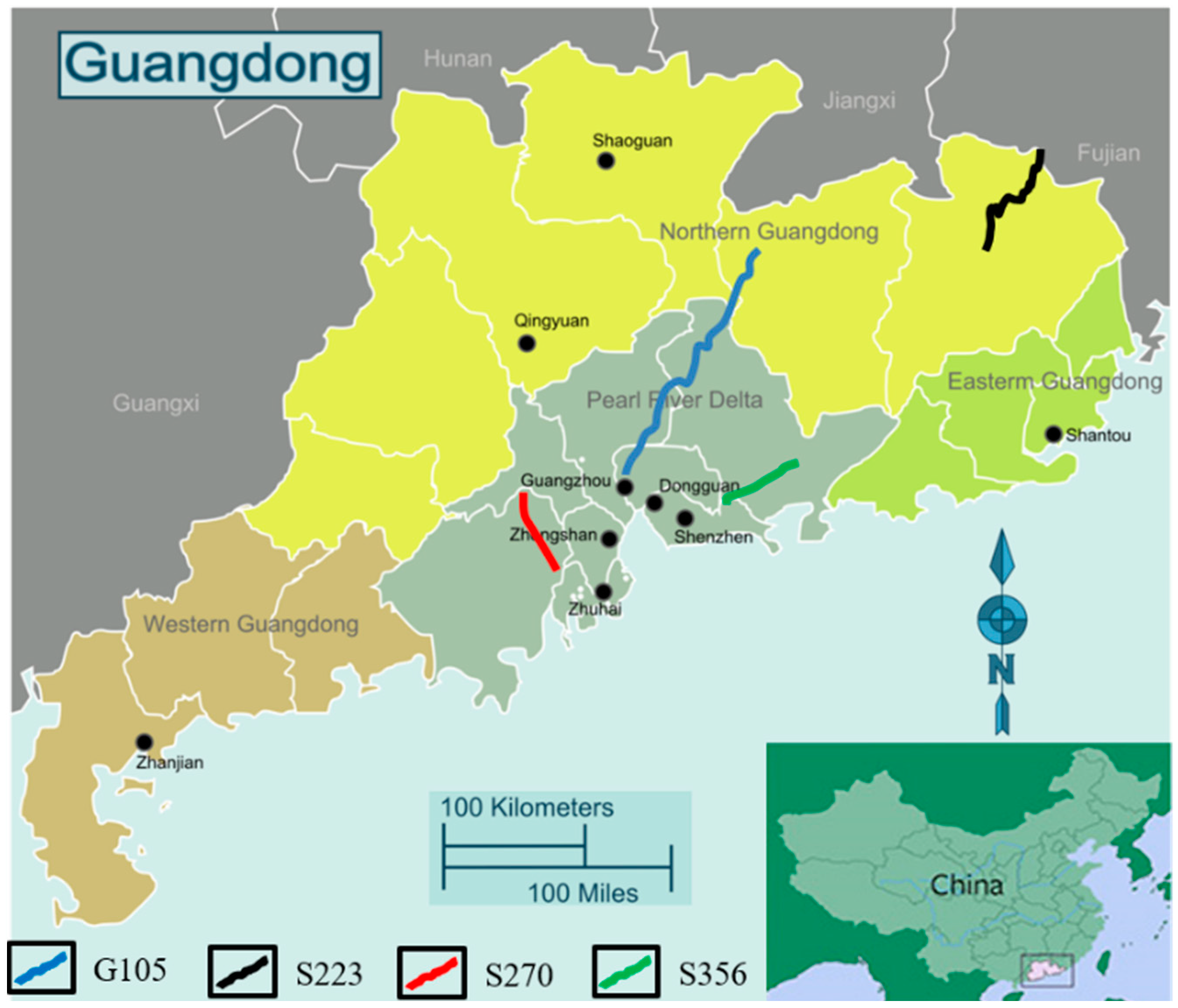
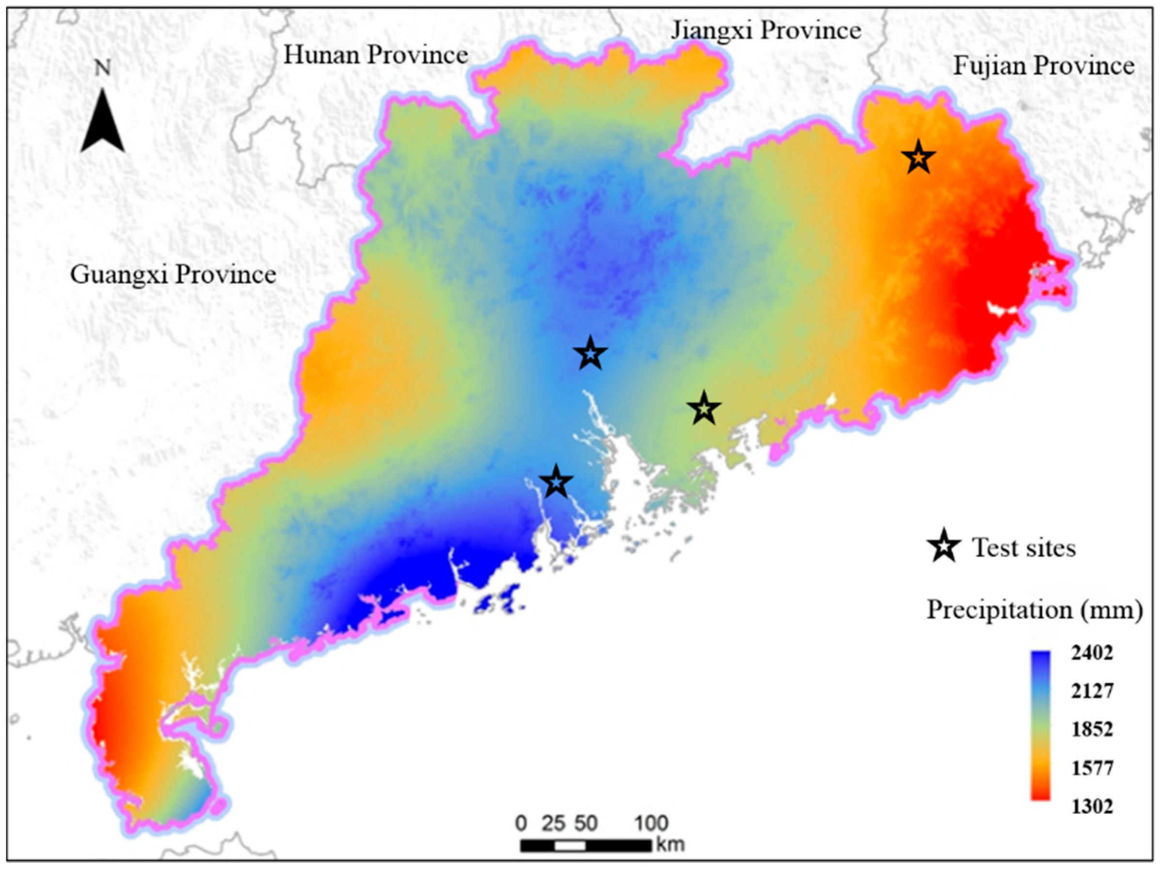
2.1. Description of the Test Area

In the first decade of the 20th century, an unprecedented upsurge of highway construction was initiated in Guangdong, China, where the economy developed rapidly, and the construction of the backbone highway network was carried out on a large scale. By 2016, most highways had been operating for approximately ten years. The subgrade performances were relatively stable during the first 10 years of the operational period, but after the 10-year operational period, subgrade distresses were aggravated by typhoons and heavy rainfall activities in recent years. Therefore, it is necessary to select typical roads for performing an effective subgrade distress investigation, evaluation, and prediction, to reasonably plan subgrade maintenance.

The locations of the four typical first-class highways that are crucial to the local highway network are given in Figure 1. Two different highway classifications are included: one National Highway (G105) and three Provincial Highways (S223, S270, and S356). (1) G105 is located in Conghua City, in the central part of Guangdong Province. The highway is located in the transitional zone from the Pearl River Delta to the mountain area in the north of Guangdong Province. The Quaternary weathered layer and residual soil along the line are relatively well developed, and the regional bedrock is mainly granite. (2) S223 is located in Meizhou City, in the northeast of Guangdong Province. This line is mainly distributed in mountainous and some hilly terrain areas. Broken silty sandstone is widely distributed along the route with developed joints and fissures. (3) S270 is located in the south–central part of Guangdong Province, adjacent to the Pearl River Delta. The terrain along the line is mainly plains, with a widely distributed soft foundation. This route is mainly located in a marine sedimentary zone, with flat terrain and developed regional water systems. The joints and fissures of the rock mass are developed, the joints are crisscrossed, and the degree of integration is poor. (4) S356 is located in Huizhou City in the southeast coast of Guangdong Province. There are numerous high and steep slopes along the line with broken weathered shale rock and soil distributed alternately. Five typical unit sections are selected from each highway, and the length of each unit section is 1 km. In total, twenty representative test sites from four highways are included: G105 from K2451 to K2456, S223 from K91 to K96, S270 from K100 to K105, and S356 from K5 to K10.

2.2. Implementation of the Subgrade Distress Investigation and Data Collection

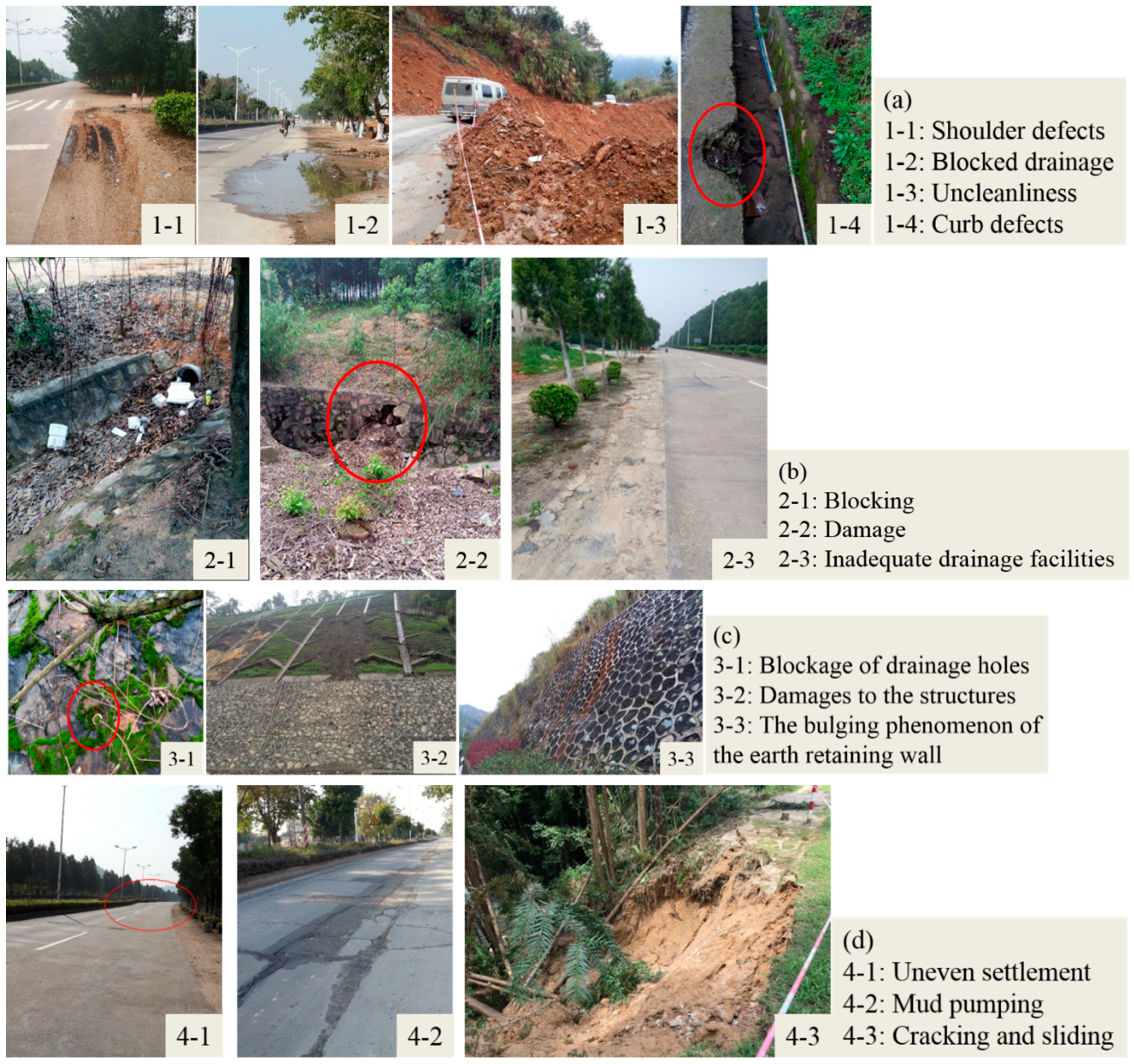
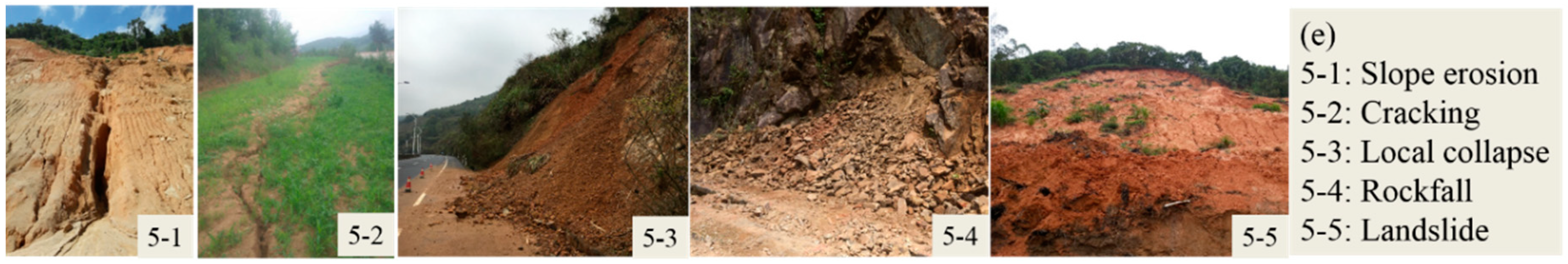
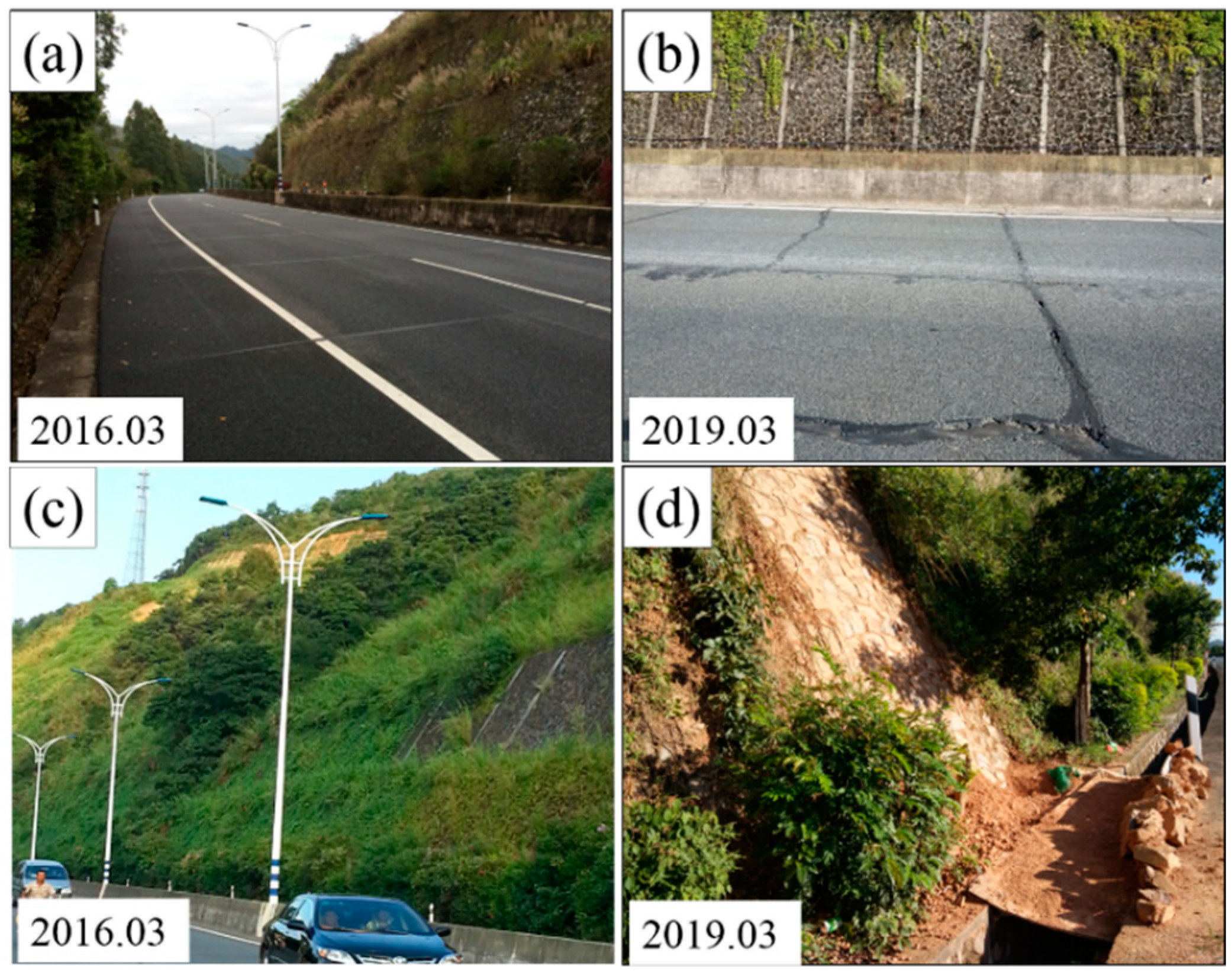
2.2.1. Investigation of the Subgrade Distresses in the Test Section

The subgrade distress investigations of the test sections began in 2016 and were conducted twice in March and September every year. Through the end of March 2019, a total of seven sets of survey data were obtained. Through the systematic distress survey conducted over three years, the typical distress forms of highway subgrade in this area are shown in Figure 2. In view of Figure 2a, there are four types of distresses that affect the performance of the shoulder, including shoulder defects, blocked drainage, uncleanliness, and curb defects. The performance of the shoulder will affect the flatness and solidity of the subgrade. At the same time, the shoulder can provide lateral support for the base and cushion of the subgrade and stabilize the structure of each layer of subgrade. Figure 2b depicts that the performance of drainage facilities has been affected, which results in poor subgrade drainage. There are three types of distresses affecting the drainage facilities: blocking, damage, and inadequate drainage facilities. When the drainage facilities are blocked, the water in the road area will not be completely and quickly discharged. This will reduce the shear strength of the soil and affect the strength and stability of the subgrade. Figure 2c illustrates the distresses of the reinforced structure. There are three types of distresses that affect the performance of the reinforced structure: blockage of drainage holes, damage to the structure, and abnormal structural stress. A reinforcement structure is used to support a natural slope or an artificial fill slope to ensure soil stability. When the reinforced structure is damaged, the structural function will decline and cause the soil to collapse or the slope to lose stability. This will negatively affect the safety of road users. As shown in Figure 2d, there are three types of distresses affecting the performance of the embankment and roadbed: uneven settlement, pumping, and cracking and sliding. The cracking of the embankment will cause rainwater to directly enter the embankment soil layer, thereby reducing the strength and resilience modulus of the embankment soil. In this situation, the stability of the subgrade is negatively affected. Figure 2e displays the distresses of the slope after rainfall. There are five types of distresses affecting the slope performance: slope erosion, cracking, local collapse, rockfall, and landslides. A slope is an important part of subgrade. The stability of the slope determines the overall function and structure of the subgrade.

2.2.2. Subgrade Distress Data Collection

The collection of subgrade distress data is based on manual surveys, which are mainly conducted through an operable visual method, supplemented by a tape measure. The basic principles of the collection process are simple, scientific, reasonable, and easy to carry out. Subgrade distresses data were collected and the determination of the deduction points are shown in

Table 1. Subgrade distresses data collection and determination of the deduction points.

Object	Distress Types	Level	Unit	Deduct Points	Definition
Road shoulder	Shoulder defects	Minor	Place	10	Shallow rutting or potholes less than 25 mm
		Severe	Place	20	Shallow rutting or potholes larger than or equal to 25 mm
	Blocked drainage	Minor	Place	10	Along the trend of subgrade, the length of blocking drainage is 5–20 m.
		Severe	Place	20	Along the trend of subgrade, the length of blocking drainage is more than 20 m
	Uncleanliness		Place	5	There are accumulated debris and weeds on the road shoulder
	Curb defects		Place	5	Loss, damage, or toppling of curbs
Drainage facilities	Blocking	Minor	Place	5	There are sundries and garbage in the drainage system. Every 10 m is one place, and less than 10 m is maintained
		Severe	Place	10	The full cross-section of the drainage system is blocked, every 10 m is one place, and less than 10 m is maintained
	Damaged		Place	5	The lining spalling damage and masonry body cracking occurred
	Inadequate drainage facilities		Km	100	One point will be deducted for every 10 m of inadequate drainage facilities, and less than 10 m is maintained
Reinforced structures	Blockage of drainage holes		Place	20	The expansion joint of the structure is used as the dividing section. When 30% or more of the drain holes have poor drainage, it is counted as one place
	Damages to the structures	Minor	Place	10	Partial foundation washout, wall voids, and slight cracks in supporting structures
		Severe	Place	20	The overall cracking, inclining, and sliding of the retaining structure appear
	Abnormal structural stress		Place	50	Judging by the instability of independent reinforced structures
Embankment and roadbed	Uneven settlement	Minor	Place	20	The height difference of uneven settlement is 30–50 mm
		Severe	Place	50	The height difference of uneven settlement is greater than 50 mm
	Pumping		Place	5	The mud gushing out of the roadbed is one place.
	Cracking and sliding		Place	50	Arc-shaped cracks along the longitudinal direction of the subgrade pose a greater threat to the safety of the subgrade
Slope	Slope erosion		Place	20	Gullies with a width and depth of 10 cm or more are counted as one place
	Cracking	Minor	Place	20	There are some vertical cracks in the side boundary of the slope
		Severe	Place	50	A tensile crack at the top of the slope
	Local collapse		Place	50	The rock and soil mass on the slope surface is loose and broken, resulting in local slope collapse
	Rockfall		Place	20	The rock mass splits and peels off, causing the gravel to roll off
	Landslide		Place	100	The overall slide of the slope causes traffic interruption

. Two distress levels (severe and minor) of the cracks were collected in the test sections. An average crack depth less than or equal to 25 cm was treated as a “minor” distress level. The levels of the other subgrade distresses follow the specification of JTG H20-2007 [33].

2.3. Evolution Process and Influencing Factors of Subgrade Distress

The climate in the investigated area is that of a subtropical monsoon, which is one of the regions with the most rainfall in China. Figure 3 shows that the area where the four roads are located has an annual rainfall that is greater than 1500 mm. Both G105 and S270 have reached 2200 mm of annual rainfall. The annual rainfall distribution is extremely uneven and the precipitation from April to September accounts for more than 80% of the whole year. Landslides, debris flow, and other geological disasters are triggered after the annual seasonal rainfall and monsoon period [34,35,36].

Figure 4 illustrates the development of two typical subgrade distresses in S223 and S270. Figure 4a,b display the performances of the embankment and roadbed in S223. As shown in Figure 4a, the embankment and roadbed were in good condition when the survey was started in March 2016. However, due to the influence of the cumulative precipitation of 2206 mm from March 2016 to March 2017, there were some longitudinal and transverse cracks on the pavement. During the follow-up of the investigation, it was found that the cracks spread faster in the period from March to September each year. This is related to the seasonal heavy rainfall in this period. Figure 4b depicts the condition at the last investigation in March 2019. Due to the infiltration of rainfall along the existing cracks, the embankment soil flowed out, resulting in the uneven settlement of the embankment. Figure 4c,d depict the slope performances of S270. As can be seen from Figure 4c, at the beginning of the investigation in March 2016, the slope was covered with vegetation and was in good condition. Unfortunately, in June and August 2018, this region was frequently impacted by tropical storms. From June 4 to 9, the region experienced continuous rainfall, with an accumulated rainfall of 807.8 mm and a maximum daily rainfall measuring more than 500 mm. As can be seen from Figure 4d, in March 2019, the last survey found that a large number of existing slopes suffered from slope erosion and local collapse.

3. Methodology

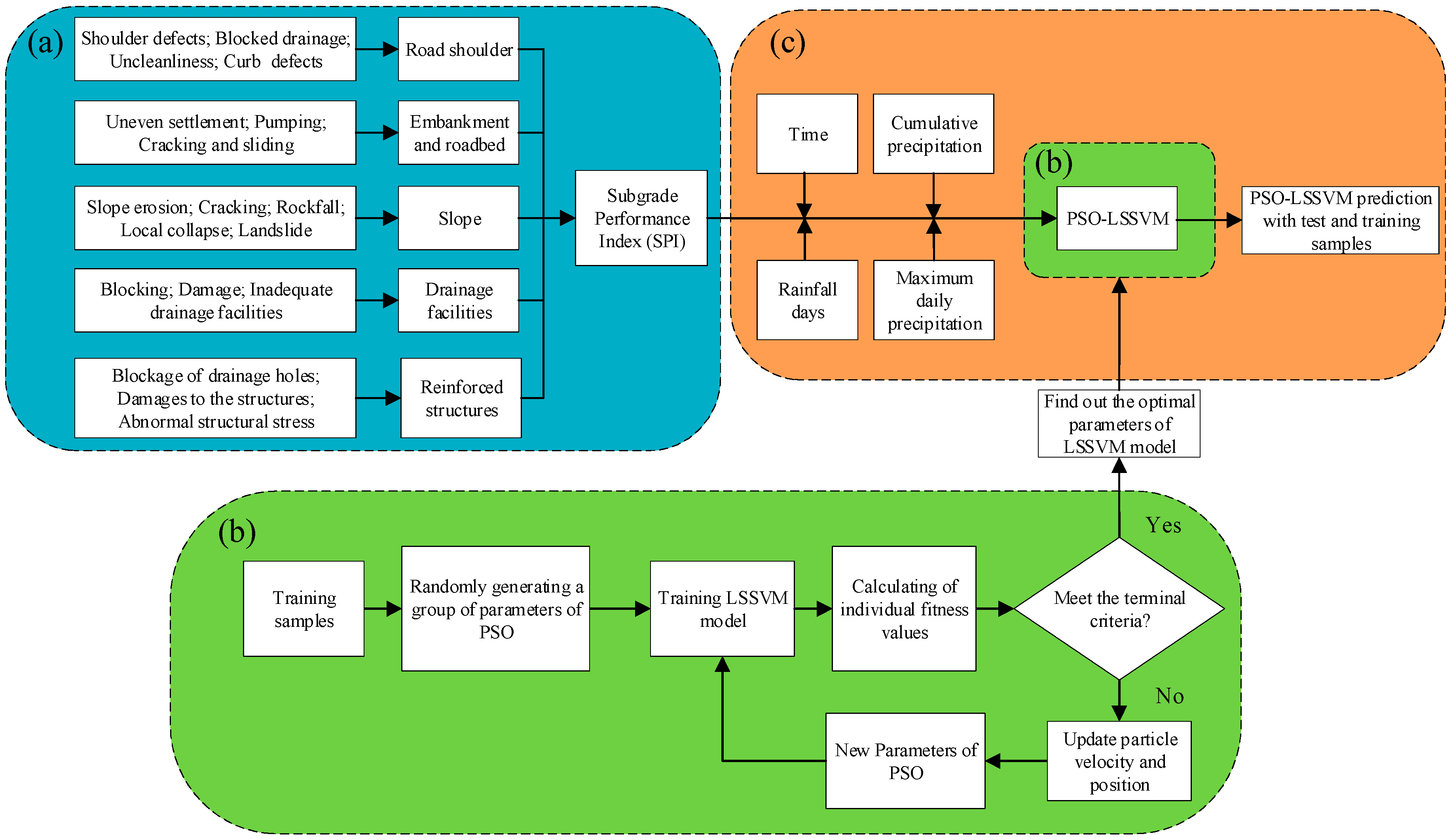
3.1. Systematic Assessment Method of the Subgrade Performance

3.1.1. Hierarchical Structure

The analytic hierarchy process (AHP), developed by Thomas Saaty in the late 1970s [37], enables the derivation of priorities or weights, as opposed to arbitrary judgment [38]. The AHP method is widely used in the sensitivity analyses of geotechnical engineering applications with high performance [39,40,41,42,43]. According to the content of the subgrade performance survey and the principle of AHP, an SPI hierarchical structure model was established. This is shown in Figure 5a. The specific subgrade distresses, such as shoulder defects, uneven settlement, slope erosion, blockage of drainage holes, and so on, are the first-level indexes. Then, the five assessment objects of the road shoulder, embankment and roadbed, slope, drainage facilities, and reinforced structures are taken as the second-level indexes. Finally, the SPI can be established for the target layer.

3.1.2. Comparison Matrix

To apply the AHP, it is necessary to decompose a complex unstructured problem into its constituent indexes, arrange these indexes in hierarchical order, assign values to subjective judgments about the relative importance of each index, and integrate these judgments to determine the priorities to be assigned to these indexes [38]. Therefore, by comparing the importance of each index in the hierarchy model, the corresponding comparison matrix A is obtained:

$$A=\left[\begin{array}{cccc}{a}_{11}& a_{12}& \dots & a_{1n}\\ a_{21}& a_{22}& \dots & a_{2n}\\ ⋮& ⋮& ⋮& ⋮\\ a_{n1}& a_{n2}& \dots & a_{nn}\end{array}\right]$$

(1)

Here, $a_{ij}$ is the importance of the comparison between index i and index j. The quantitative method of 3-level importance is adopted, and the corresponding values are 0–2, which represents important, unimportant, and equally important. When index i is more important than index j, $a_{ij}$ is “2”; when index i is less important than index j, $a_{ij}$ is “0”; when i and j are equally important, $a_{ij}$ is “1”.

3.1.3. Building the Judgment Matrix

According to the comparison matrix A, the corresponding judgment matrix C is constructed as follows:

$$r_i={\displaystyle \sum _{l=1}^n{a}_{il}}$$

(2)

$$b_{ij}=\{\begin{array}{cc}{r}_i-r_j,& r_i>r_j\\ 1,& r_i=r_j\\ {(r_j-r_i)}^{-1},& r_i<r_j\end{array}$$

(3)

$$c_{ij}=\frac{\sqrt[n]{{\Pi }_{l=1}^n{b}_{il}}}{\sqrt[n]{{\Pi }_{l=1}^n{b}_{lj}}}$$

(4)

$$C={(c_{ij})}_{n\times n}$$

(5)

where r_i is the ranking element of importance, b_ij is the result of comparing the ranking elements with each other, c_ij is the elements of the judgment matrix C, and i, j = 1, 2, …, n.

3.1.4. Calculation of the Index Weights

According to the judgment matrix C, the weighted values of each index are calculated as follows:

$${\overline{\omega }}_i=\sqrt[n]{{\displaystyle \prod _{j=1}^n{c}_{ij}}}\underset{\begin{array}{c}\mathrm{normalization}\\ \mathrm{processing}\end{array}}{\to }{\omega }_i=\frac{{\overline{\omega }}_i}{{\displaystyle {\sum }_{j=1}^n{\overline{\omega }}_j}}$$

(6)

where ${\omega }_i$ is the final weight value.

3.1.5. Application of the Weight Value

According to the deduction standard in Table 1, one must first obtain the distress deduction point (DP), then the SPI_i of each index in the second level, and the target of the SPI can be constructed according to the following formula:

$$SP{I}_i=100-{\displaystyle \sum _{j=1}^m(D{P}_{ij}\times {\omega }_{ij}})\underset{\mathrm{integration}}{\to }SPI={\displaystyle \sum _{i=1}^5(SP{I}_i}\times {\omega }_i)$$

(7)

where DP_ij is an accumulated deduction point of distress j of index i in the second level, ${\omega }_{ij}$ is the weight value of distress, j, of index i in the second level, and ${\omega }_i$ is the weight value of index i in the second level.

3.2. Principles of the PSO–LSSVM Model

3.2.1. Least Squares Support Vector Machine (LSSVM)

The LSSVM is a supervised learning method that is not only used to analyze data and identify patterns, but is also used for classification and regression analyses. The LSSVM applies equality constraints to inequality constraints of the SVM, thereby converting the quadratic optimization problem into a system of linear equations that is based on the least squares criterion.

${\left(x_i,y_i\right)}_{i=1}^l$ is a dataset of l samples where the input data, x_i, are a D-dimensional input vector and y_i denotes the target data. The regression estimation function of the LSSVM is as follows:

$$f(x)=w^T\phi (x)+b$$

(8)

where $f(x)$ denotes the predictive values, $\phi (x)$ is the nonlinear mapping from the input space to the output space, and w and b are the coefficients to be adjusted.

Transforming the regression estimation function into a function minimization problem using the slack variable e is performed by the following:

$$\mathrm{Minimize} J(w,e)=\frac{1}{2}{\Vert w\Vert }^2+\frac{1}{2}\gamma {\displaystyle \sum _{i=1}^l{e}_i^2}$$

(9)

$$\mathrm{Subject} \mathrm{to} y_i=w^T\phi (x_i)+b+e_i,i=1,\dots ,l$$

(10)

where $\gamma$ is a regularization parameter.

To solve the optimization problem of the LSSVM, the Lagrangian function is constructed as follows:

$$L(w,b,e,\alpha )=J(w,e)-{\displaystyle \sum _{i=1}^l{\alpha }_i}\left(w^T\phi (x_i)+b+e_i-y_i\right)$$

(11)

where ${\alpha }_i$ is the Lagrange multiplier. The conditions for optimality are given by:

$$\{\begin{array}{c}\frac{\partial L}{\partial w}=0\to w={\displaystyle \sum _{i=1}^l{\alpha }_i\phi (x_i)}\hfill \\ \frac{\partial L}{\partial b}=0\to {\displaystyle \sum _{i=1}^l{\alpha }_i}=0\hfill \\ \frac{\partial L}{\partial e_i}=0\to {\alpha }_i=\gamma e_i\hfill \\ \frac{\partial L}{\partial {\alpha }_i}=0\to w^T\phi (x_i)+b+e_i=y_i\hfill \end{array}$$

(12)

According to the Karush–Kuhn–Tucker optimum condition, the following linear equation set is obtained:

$$\left[\begin{array}{cc}0& I_l^T\\ I_l& K+{\gamma }^{-1}{I}_l\end{array}\right]\left[\begin{array}{c}b\\ \alpha \end{array}\right]=\left[\begin{array}{c}0\\ y\end{array}\right]$$

(13)

where $I_l={\left[1,1,\dots ,1\right]}^T$, $\alpha ={\left[{\alpha }_1,{\alpha }_2,\dots ,{\alpha }_l\right]}^T$,$y={\left[y_1,y_2,\dots ,y_l\right]}^T$, I_l is an $l\times l$ identity matrix, K is a kernel function with $l\times l$ symmetric matrix, and $K_{ij}=\phi {(x_i)}^T\phi (x_i)=K(x_i,x_j)$.

There are three commonly used kernel functions available: the linear kernel, polynomial kernel, and radial basis kernel function (RBF). In this paper, the radial basic function (RBF) is used as the kernel function of the LSSVM model because of its wide convergence domain and excellent nonlinear mapping performance [44]. Finally, the regression function of the LSSVM prediction model can be obtained by:

$$f(x)=w^T\phi (x)+b={\displaystyle \sum _{i=1}^l{\alpha }_{i}K(x,x_i)}+b$$

(14)

3.2.2. Parameter Selection of the LSSVM Using PSO

When the kernel function of the LSSVM is RBF, there are two parameters that need to be determined by users in order to determine the efficiency and generalization performance of the LSSVM: the regularization parameter, $\gamma ;$ and the kernel function width, $\sigma$. Inspired by the social interaction model of birds foraging, PSO uses swarm intelligence to achieve the goal of optimization. A particle is used to simulate the individual birds. Particles have only two attributes: speed and position. Speed represents the speed of movement, and position represents the direction of movement. The optimal solution where each particle searches individually is called individual extremum, and the optimal individual extremum in this particle swarm is the current global optimal solution. The speed and position are updated through constant iterations. Finally, the optimal solution that satisfies the termination condition is obtained. Therefore, the PSO is chosen to search for the optimal parameters in this paper.

The subgrade is a multidimensional dynamic system affected by multiple factors, such as rainfall and time during operation. The test section is located in the coastal area of Southeast China, with an obvious subtropical monsoon climate. Impacted by long-term rainfall and short-term rainstorms from June to August every year, the subgrade distresses easily accumulate and form mutations. However, in the months with less rainfall, the subgrade maintains a relatively stable state. Therefore, the influencing factors of rainfall and time are considered to be the keys to predicting the SPI. The implementation procedure of the overall PSO–LSSVM model is shown in Figure 5. In order to verify the prediction accuracy of the model, the Mean Square Error (MSE) is employed to obtain the fitness value, which is shown as:

$$MSE=\frac{1}{N}{\displaystyle \sum _{i=1}^N{(y_i-{\widehat{y}}_i)}^2}$$

(15)

where $y_i$ and ${\widehat{y}}_i$ are the actual and predicted value, respectively. N is the number of samples for training.

4. SPI Prediction and Application

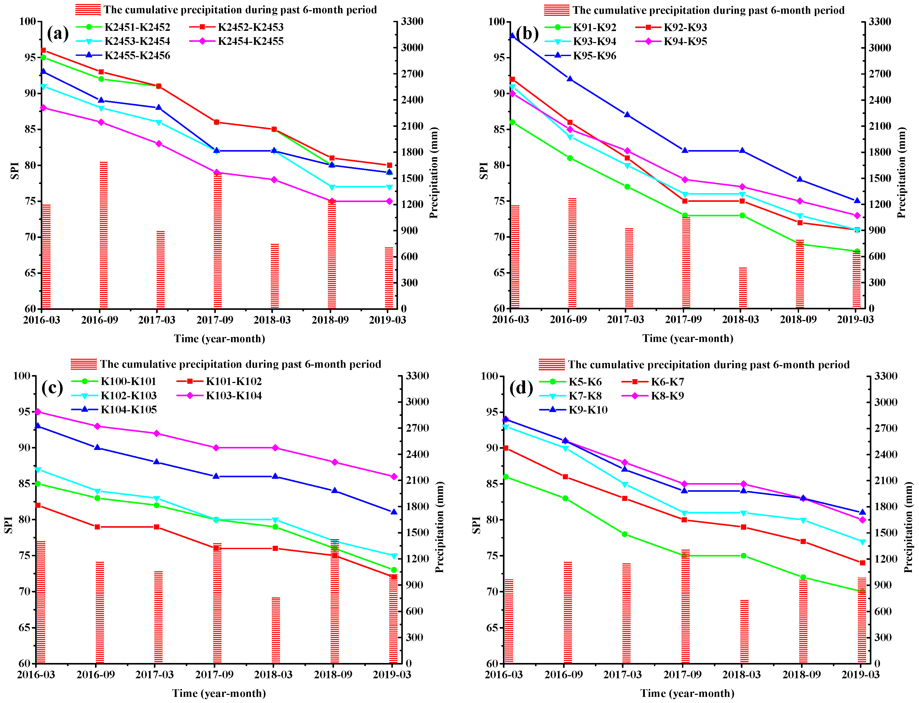
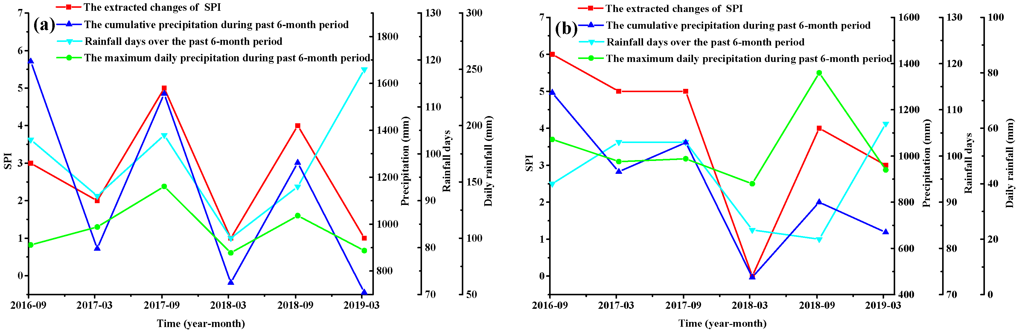
4.1. Analysis of the SPI

According to the AHP method, we issued an electronic questionnaire to 10 experts and scholars of highway maintenance management, aiming to quantitatively rank and analyze the importance of each index. Since the importance of index judgment given by individual respondents is different, it is necessary to calculate all the values of each index separately and take the weighted average value as the element in the initial judgment matrix to obtain a reasonable judgment matrix after multiple consistency tests and adjustments [43]. The weights of the five assessment objects in the second-level indexes are first obtained by establishing a judgment matrix. Then, the first-level judgment matrix is established for the specific subgrade distresses, which appear in the second-level objects. Finally, the assessment system of the subgrade distress is shown in

Table 2. The assessment system of the subgrade distress.

Second-Level Indexes	Index Weight	First-Level Indexes	Index Weight	Second-Level Indexes	Index Weight	First-Level Indexes	Index Weight
Embankment and roadbed	0.27	Uneven settlement	0.376	Road shoulder	0.08	Shoulder defects	0.255
		Pumping	0.221			Blocked drainage	0.413
		Cracking and sliding	0.403			Uncleanliness	0.235
Drainage facilities	0.10	Blocking	0.441			Curb defects	0.097
		Damage	0.347	Slope	0.36	Slope erosion	0.135
		Inadequate drainage facilities	0.212			Cracking	0.065
Reinforced structures	0.19	Blockage of drainage holes	0.153			Local collapse	0.078
		Damages to the structures	0.505			Rockfall	0.283
		Abnormal structural stress	0.342			Landslide	0.439

. A landslide not only interrupts traffic for a long time, but also directly causes casualties and property losses. Therefore, “landslide” is the distress type with the highest weighting value among all the distress types. Through the assessment system, the SPI results of twenty sites spread over four highways from March 2016 to March 2019 are obtained (Figure 6). As shown in Figure 6, subgrade distress is an irreversible process that, like the evolution of a landslide, exhibits an open state [45], and the development of cracks ranges from small-scale local cracks to large-scale regional cracks [46]. Therefore, the subgrade distress of the twenty test sites accumulated on top of the previous ones, resulting in the decrease in the SPI. Additionally, the rate of SPI decline was generally the highest from March to September, which was the most concentrated and abundant period of rainfall. From October to February of the following year, the SPI of most test sites remained stable, which indicated that the change in the SPI was highly correlated with rainfall.

The five test sites selected from the same highway have a similar investigation duration and frequency. Additionally, different test sites on the same highway exhibit similar rates of SPI decline (Figure 6). Therefore, a typical section is selected to represent each highway in this study. The relationship between the extracted changes of the SPI and accumulated precipitation, maximum daily precipitation, and rainfall days over the past 6-month period are provided (Figure 7). Using the Pearson Correlations (r) analysis method to evaluate the strength of a linear relationship between two variables [47], the Pearson Correlation, r, between the SPI changes and the impact factors is shown in

Table 3. Pearson Correlations between the SPI changes and impact factors.

Sites	Cumulative Precipitation	Rainfall Days	Maximum Daily Precipitation
K2452–K2453 of G105	0.826	0.232	0.890
K95–K96 of S223	0.935	0.411	0.375
K103–K104 of S270	0.802	0.550	0.159
K9–K10 of S356	0.874	0.815	0.603

. Generally, $r\le 0.39$ represents weak correlations, r between 0.40 and 0.69 represents moderate correlations, and r between 0.70 and 1 represents strong or high correlations [48].

The r between the SPI changes of G105 and the cumulative precipitation and maximum daily precipitation is above 0.8, demonstrating a strong correlation (Figure 7a and Table 3). During the investigation period, the maximum accumulated precipitation of G105 in half a year reaches 1694 mm. This occurs from March to September 2016. The maximum daily precipitation occurs in June 2017, reaching 146 mm. The rain intensity level is heavy rain (http://www.cma.gov.cn/). Normally, the rainy season is from March to August every year and annual rainfall is mainly concentrated in this period. The accumulated precipitation in the rainy season is generally about twice as high as it is in other months. In addition, this highway is built along the mountainous area, where the integrated granite stratum is widely distributed, so that the decrease in SPI is small.

As can be seen from Figure 7b,c and Table 3, the r between the SPI changes of S223 and S270 and the cumulative precipitation is above 0.8. The two highways are built along the river. Under the condition of extreme rainfall, the embankment along the river is prone to erosion, resulting in the overall sliding of the embankment [49,50]. Additionally, the cracks caused by the uneven settlement of the embankment and the shrinkage cracks during the summer months allow the formation of positive pore water pressure at a shallow depth and trigger embankment failure [51].

Figure 7d and Table 3 show that the correlation between the SPI changes of S356 and the cumulative precipitation and rainfall days is strong. Along the line of S356, there are many double-decked slopes, the surface layer is weathered residual soil, and the residual soil slopes are very sensitive to short-term heavy rainfall [52].

Moreover, this line is located in the coastal area, and there are typhoons throughout the year. Typhoons are often accompanied by short-term heavy rains, causing a large number of slope erosion and local collapse disasters.

Again, the evolution of subgrade distress is not only affected by external rainfall factors, but also by internal time factors that affect subgrade ancillary structures (such as retaining walls, anchor cables, anti-slide piles, etc.). The same is true for the multi-stage characteristic evolution process shown by landslide disasters [19]. The response process of the subgrade distress evolution to the same external factors may be different. When the ancillary structures of the subgrade are in a stable stage, even a strong influence from external factors can hardly cause subgrade distress. In contrast, when the ancillary structures begin to age after a certain period of time, which leads to a decline in anti-sliding ability, even slight disturbances may cause subgrade damage. Therefore, the time factor is considered as the internal factor of the SPI.

4.2. Building the PSO–LSSVM Model

Based on the previous study, the time series of four influencing factors, including the three external triggers (accumulated precipitation, maximum daily precipitation and rainfall days over the past 6-month period) and one internal factor (time), are taken as the input parameters. The SPI is regarded as the output parameter to establish the PSO–LSSVM model. The SPI values from March 2016 to March 2018 (71% of the database) are chosen as the training samples and SPI dates from September 2018 to March 2019 (29% of the database) are chosen as the test samples to verify model reliability. During the sample data preprocessing, all the factors and the SPI are converted to a [0,1] format. Then, the following values of the parameters to be optimized in LSSVM into the solution of PSO are encoded: the regularization parameter is $\gamma$ = [0.1, 1.0 × 10⁶] and the kernel function width is $\sigma$ = [0.1, 100]. The maximum number of evolutionary iterations is 300, the population of the particle swarm is 30, and the inertia weight is decreased linearly from about 1.0 to 0.4. The optimized parameters, $\gamma$ and $\sigma ,$ for the PSO–LSSVM model are shown in

Table 4. Optimized parameters of the PSO–LSSVM model for the four test sites.

Parameters	K2452–K2453 of G105	K95–K96 of S223	K103–K104 of S270	K9–K10 of S356
$\gamma$	14.743	0.1	1.0 × 106	11.455
$\sigma$	1.922	7.672	57.009	1.313

. To evaluate the predictive performance of the model, the conventional models, including Grid-SVM [25] and GA-SVM [22,53,54], are compared with the PSO–LSSVM model. The comparison and accuracy of the prediction values are shown in Figure 8.

As shown in Figure 8, three models (PSO–LSSVM, Grid-SVM, and GA-SVM) have achieved good SPI prediction results for the four test sites, with the PSO–LSSVM model demonstrating the highest level of accuracy. It was especially accurate in predicting the SPI of the three Provincial Highways, likely because there is more traffic flow on the National Highway than on the Provincial Highways, which increased the difficulty of building the SPI prediction model. In K95–K96 of S223, the SPI declined sharply, and the rate of SPI decline was greater than that of the other three test sites. In relation to the controlling factors, the PSO–LSSVM still showed a good prediction with the MSE of 0.47. Therefore, the PSO–LSSVM model can better reflect the relationship between the impact factors and the SPI, and it is capable of predicting both ’gently decreasing type and rapid decreasing type SPIs.

4.3. Application for the Date of the SPI

The following method was used to predict the SPI values in the near future. Based on the PSO–LSSVM model, the time series of four influencing factors and the SPI from March 2016 to March 2019 are chosen as the training samples. The SPI from September 2019 is predicted by taking the cumulative precipitation, maximum daily precipitation, and rainfall days from March to September 2019 as input parameters. The predicted results are given in

Table 5. Predicted SPI results for September 2019.

Sites	Cumulative Precipitation (mm)	Rainfall Days	Maximum Daily Precipitation (mm)	Predictive Values for September 2019
K2452–K2453 of G105	1720	114	108	76.82
K95–K96 of S223	1333	109	76	70.16
K103–K104 of S270	1914	116	123	81.70
K9–K10 of S356	1363	90	63	78.96

for the different test sites. The relevant national standards of China can be referenced to meet the actual requirements of subgrade maintenance [33]. Four subgrade classification levels (excellent, good, medium, poor) are collected in the SPI test sites. The values range from 0 (poor) to 100 (excellent). For a SPI between 90 and 100, the subgrade is classified as excellent; a SPI of 80–89 is classified as good; a SPI of 70–79 is classified as medium; a SPI less than 60 is considered poor.

As can be seen from Table 5, the SPI of the K95–K96 section of S223 is the smallest. S223 was opened to traffic in May 2007. After twelve years of operation, a large number of subsidence, cracks, and other distresses have appeared in the subgrade. In addition, by predicting the subgrade performances of other sections of this highway, most of the SPI values will be in the middle or below the classification value in September 2019, which poses a great risk to driving safety. Therefore, it is necessary to take corresponding maintenance measures based on the different SPI values. Figure 9 shows the impact of reasonable treatment measures taken on subgrades with various SPI values. The preventive maintenance treatment is applied before the SPI drops below 70. Preventive maintenance is a proactive approach that systematically looks for opportunities to eliminate small problems before they become serious. This concept was first utilized for pavement, and has been widely used [55,56,57]. Although preventive maintenance treatments do not significantly improve the load-carrying capacity of subgrade, they do improve the level of service and extend the service life [58]. When the SPI is less than 70 and greater than or equal to 60, the subgrade requires maintenance and rehabilitation. When the SPI is less than 60, there is a large-scale disease or landslide on the subgrade. In this situation, overhaul or emergency disposal measures should be taken. In order to guide and verify the applicability of this definition, in the first half of 2019, technical personnel within the research institute of the Ministry of Highway Transport carried out a comprehensive inspection on the road section, and formulated a comprehensive maintenance plan for the whole section.

The other three highways were newly built or reconstructed between 2008 and 2010, and as such, they have not yet reached the critical point for preventive maintenance. However, the life-cycle decision-making for preventive maintenance of a subgrade needs to be carried out and included in the annual management cycle. This process includes budgeting, planning, and implementation activities. Figure 10 shows the life-cycle decision-making framework for preventive maintenance. Through the subgrade life-cycle decision-making system, the maintenance management department can specifically determine which subgrade sections require preventive maintenance (the right sites). This identifies the subgrade preventive maintenance needs in a timely manner (the right time), and, finally, it selects the most favorable treatment method (the right treatment).

5. Conclusions

This study focused on the performance of highway subgrades over their whole life-cycle during the operation period. It selected 20 test sites across 4 typical highways to carry out distress surveys for up to 3 years. Moreover, the assessment and prediction of subgrade performances were carried out. The following conclusions were obtained:

(1)

The development trend of subgrade distress is affected by internal factors. External factors, such as rainfall, directly cause the formation of subgrade distresses. Therefore, the relationships between the internal and external factors are important when analyzing the evolution mechanism of subgrade distress.

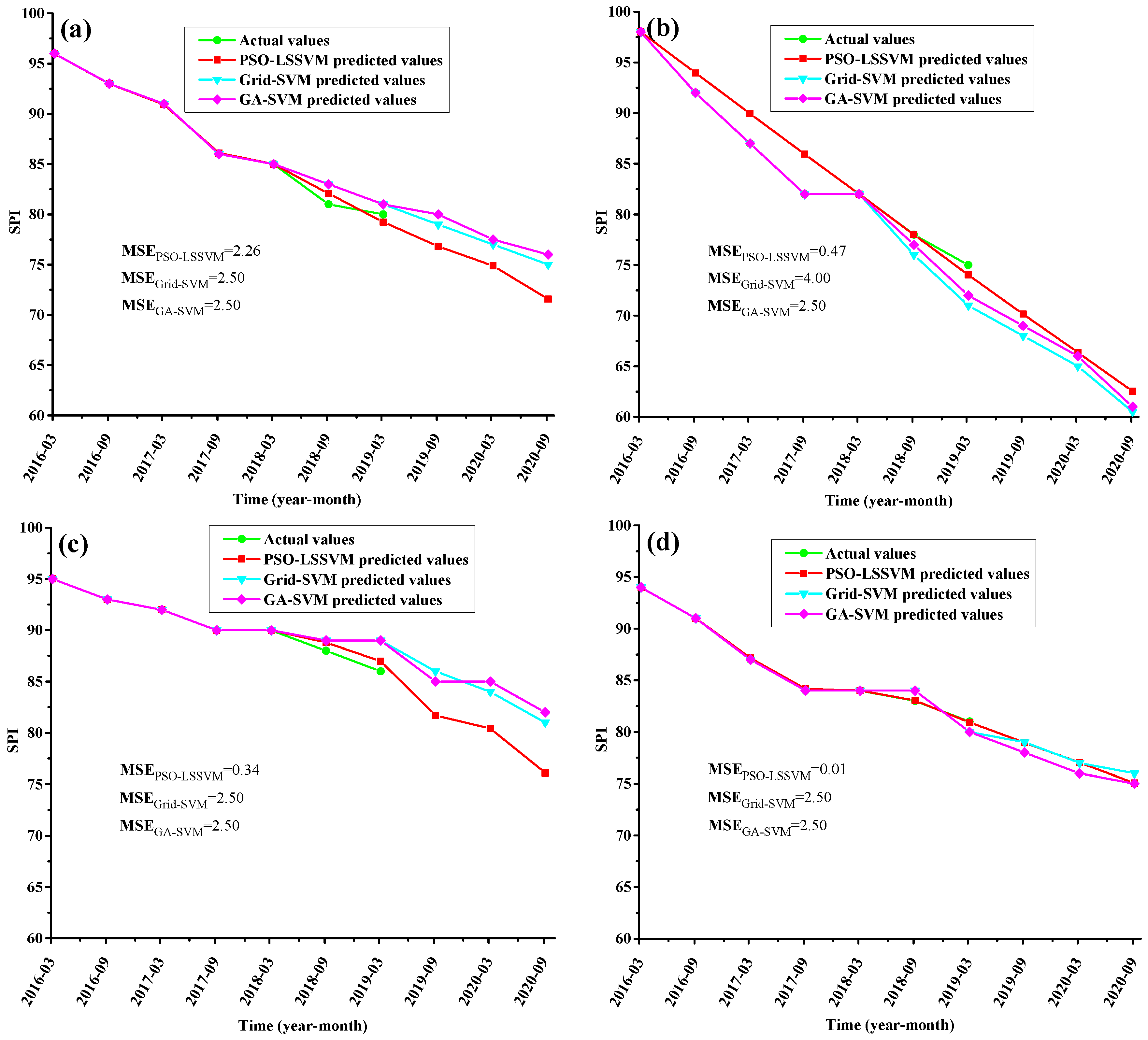
(2)

The results of the SPI calculations show that the prediction accuracy of the SPI prediction model based on PSO–LSSVM is better than the prediction accuracy of the other two models, which are based on Grid-SVM and GA-SVM. In addition, the PSO–LSSVM model accurately predicts both the gently decreasing type and rapidly decreasing type of SPI.

(3)

The prediction accuracy of provincial highways is higher than that of the national highway. This is mainly due to the large traffic volume on the national highway and the frequent occurrence of overloaded trucks, which result in redundant damage to the subgrade, thus increasing the difficulty of SPI prediction.

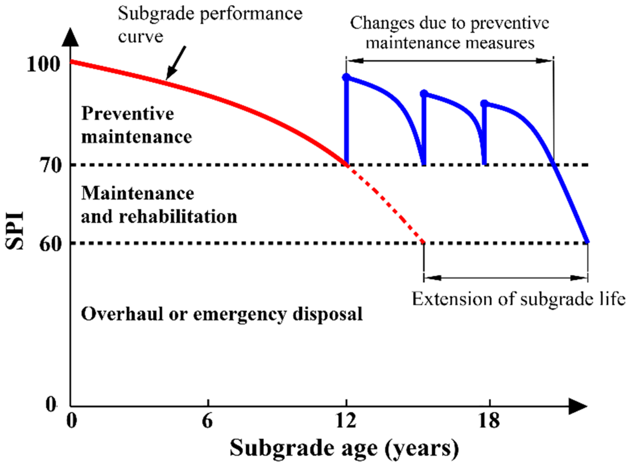
(4)

According to the SPI, the subgrade is divided into four levels. Corresponding maintenance and treatment measures are taken for different levels. Preventive maintenance is applied before the SPI drops below 70.

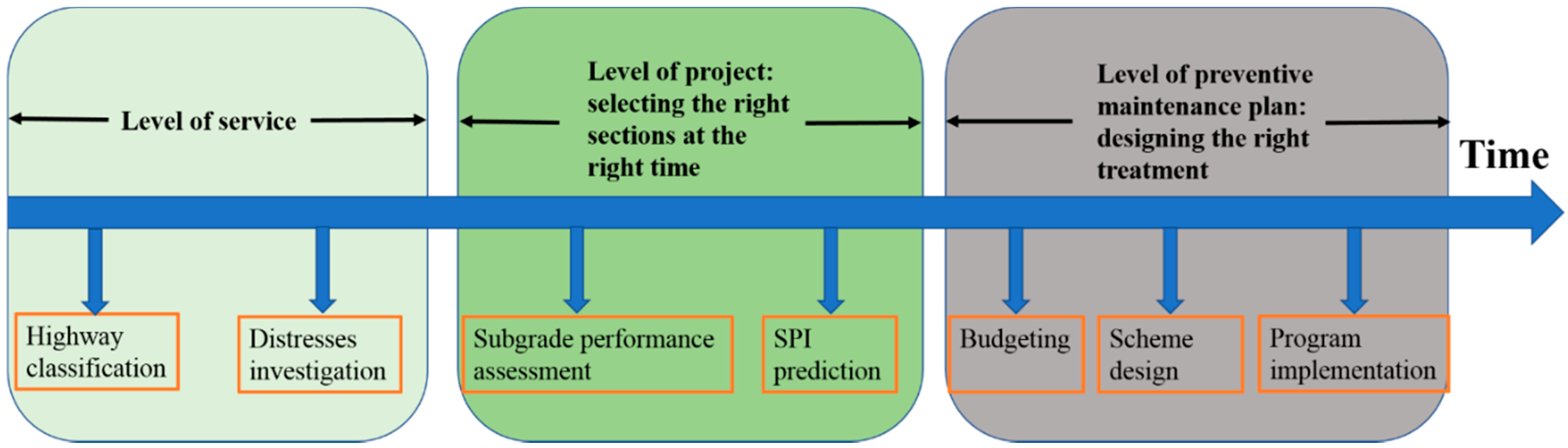
(5)

The establishment of a subgrade performance assessment–prediction–maintenance–management architecture framework provides a clear method for road maintenance managers to reasonably lay out the subgrade life-cycle assessment decision system.

References

1. Wang, S.G.; Song, X.G. Maintenance and Reinforcement of Highway Subgrade; China Communications Press Co. Ltd.: Beijing, China, 2010. [Google Scholar]
2. Zhang, L.; Wang, Y.M. Analysis on the Technology of Highway Subgrade Disease Prevention and Maintenance in Guangdong Province. Adv. Mater. Res. 2015, 1065–1069, 737–743. [Google Scholar] [CrossRef]
3. Zang, Y.Y.G. High Grade Highway Subgrade Disease Analysis and Prevention and Control Technology; China Communications Press: Beijing, China, 2007. [Google Scholar]
4. Ministry of Transport of the People’s Republic of China. Technical Specifications for Maintenance of Highway Subgrade; Volume JTG 5150—2020; China Communications Press: Beijing, China, 2020.
5. Yang, J.; Lei, L.I.; Ming, W.U.; Jiang, Z.M.; Yan, Z.L. Analysis on Type and Genesis of Subgrade Diseases of Highway in Mountainous Area. Subgrade Eng. 2012, 6. [Google Scholar]
6. Liu, F.J.; Jian, L.U.; Zhang, G.Q.; Xiang, Q.J. Evaluation Approach of Expressway Subgrade Maintenance. J. Highw. Transp. Res. Dev. 2006, 5. [Google Scholar]
7. Raj, M.; Sengupta, A. Rain-triggered slope failure of the railway embankment at Malda, India. Acta Geotech. 2014, 9, 789–798. [Google Scholar] [CrossRef]
8. Sun, H.-Y.; Pan, P.; Lü, Q.; Wei, Z.-L.; Xie, W.; Zhan, W. A case study of a rainfall-induced landslide involving weak interlayer and its treatment using the siphon drainage method. Bull. Eng. Geol. Environ. 2018, 78, 4063–4074. [Google Scholar] [CrossRef]
9. Lu, N.; Wayllace, A.; Oh, S. Infiltration-induced seasonally reactivated instability of a highway embankment near the Eisenhower Tunnel, Colorado, USA. Eng. Geol. 2013, 162, 22–32. [Google Scholar] [CrossRef]
10. Lou, Z.; Gunaratne, M.; Lu, J.J.; Dietrich, B. Application of Neural Network Model to Forecast Short-Term Pavement Crack Condition: Florida Case Study. J. Infrastruct. Syst. 2001, 7, 166–171. [Google Scholar] [CrossRef]
11. Chen, Y.; Davalos, J.F.; Ray, I. Durability Prediction for GFRP Reinforcing Bars Using Short-Term Data of Accelerated Aging Tests. J. Compos. Constr. 2006, 10, 279–286. [Google Scholar] [CrossRef]
12. Micelli, F.; Nanni, A. Durability of FRP rods for concrete structures. Constr. Build. Mater. 2004, 18, 491–503. [Google Scholar] [CrossRef]
13. Mori, Y.; Ellingwood, B.R. Reliability-Based Service-Life Assessment of Aging Concrete Structures. J. Struct. Eng. 1993, 119, 1600–1621. [Google Scholar] [CrossRef]
14. Zhu, X.; Ma, S.-Q.; Xu, Q.; Liu, W.-D. A WD-GA-LSSVM model for rainfall-triggered landslide displacement prediction. J. Mt. Sci. 2018, 15, 156–166. [Google Scholar] [CrossRef]
15. Kang, F.; Li, J.-S.; Li, J.-J. System reliability analysis of slopes using least squares support vector machines with particle swarm optimization. Neurocomputing 2016, 209, 46–56. [Google Scholar] [CrossRef]
16. Xue, X.; Yang, X.; Chen, X. Application of a support vector machine for prediction of slope stability. Sci. China Technol. Sci. 2014, 57, 2379–2386. [Google Scholar] [CrossRef]
17. Li, S.-J.; Zhao, H.-B.; Ru, Z.-L. Deformation prediction of tunnel surrounding rock mass using CPSO-SVM model. J. Cent. South Univ. 2012, 19, 3311–3319. [Google Scholar] [CrossRef]
18. Rahbarzare, A.; Azadi, M. Improving prediction of soil liquefaction using hybrid optimization algorithms and a fuzzy support vector machine. Bull. Eng. Geol. Environ. 2019, 78, 4977–4987. [Google Scholar] [CrossRef]
19. Zhou, C.; Yin, K.; Cao, Y.; Ahmed, B. Application of time series analysis and PSO–SVM model in predicting the Bazimen landslide in the Three Gorges Reservoir, China. Eng. Geol. 2016, 204, 108–120. [Google Scholar] [CrossRef]
20. Vapnik, V.N. The Nature of Statistical Learning Theory; Springer: Berlin/Heidelberg, Germany, 2000. [Google Scholar]
21. Su, C.; Wang, L.; Wang, X.; Huang, Z.; Zhang, X. Mapping of rainfall-induced landslide susceptibility in Wencheng, China, using support vector machine. Nat. Hazards 2015, 76, 1759–1779. [Google Scholar] [CrossRef]
22. Li, X.Z.; Kong, J.M. Application of GA–SVM method with parameter optimization for landslide development prediction. Nat. Hazards Earth Syst. Sci. 2014, 14, 525–533. [Google Scholar] [CrossRef] [Green Version]
23. Suykens, J.A.K.; Vandewalle, J. Least Squares Support Vector Machine Classifiers. Neural Process. Lett. 1999, 9, 293–300. [Google Scholar] [CrossRef]
24. Pourghasemi, H.R.; Rahmati, O. Prediction of the landslide susceptibility: Which algorithm, which precision? Catena 2018, 162, 177–192. [Google Scholar] [CrossRef]
25. Miao, F.; Wu, Y.; Xie, Y.; Li, Y. Prediction of landslide displacement with step-like behavior based on multialgorithm optimization and a support vector regression model. Landslides 2017, 15, 475–488. [Google Scholar] [CrossRef]
26. Tan, X.; Yu, F.; Zhao, X. Support vector machine algorithm for artificial intelligence optimization. Clust. Comput. 2018, 22, 15015–15021. [Google Scholar] [CrossRef]
27. Gao, X.; Hou, J. An improved SVM integrated GS-PCA fault diagnosis approach of Tennessee Eastman process. Neurocomputing 2016, 174, 906–911. [Google Scholar] [CrossRef]
28. Kavzoglu, T.; Kutlug Sahin, E.; Colkesen, I. Selecting optimal conditioning factors in shallow translational landslide susceptibility mapping using genetic algorithm. Eng. Geol. 2015, 192, 101–112. [Google Scholar] [CrossRef]
29. Guo, X.C.; Yang, J.H.; Wu, C.G.; Wang, C.Y.; Liang, Y.C. A novel LS-SVMs hyper-parameter selection based on particle swarm optimization. Neurocomputing 2008, 71, 3211–3215. [Google Scholar] [CrossRef]
30. Poli, R.; Kennedy, J.; Blackwell, T. Particle swarm optimization. Swarm Intell. 2007, 1, 33–57. [Google Scholar] [CrossRef]
31. Tang, X.; Hong, H.; Shu, Y.; Tang, H.; Li, J.; Liu, W. Urban waterlogging susceptibility assessment based on a PSO-SVM method using a novel repeatedly random sampling idea to select negative samples. J. Hydrol. 2019, 576, 583–595. [Google Scholar] [CrossRef]
32. Wei, Z.-L.; Shang, Y.-Q.; Sun, H.-Y.; Xu, H.-D.; Wang, D.-F. The effectiveness of a drainage tunnel in increasing the rainfall threshold of a deep-seated landslide. Landslides 2019, 16, 1731–1744. [Google Scholar] [CrossRef]
33. Department of Transportation. Highway Performance Assessment Standards; Volume JTG H20-2007; China Communications Press: Beijing, China, 2007.
34. Oh, S.; Lu, N. Slope stability analysis under unsaturated conditions: Case studies of rainfall-induced failure of cut slopes. Eng. Geol. 2015, 184, 96–103. [Google Scholar] [CrossRef]
35. Yang, K.-H.; Uzuoka, R.; Thuo, J.N.; Lin, G.-L.; Nakai, Y. Coupled hydro-mechanical analysis of two unstable unsaturated slopes subject to rainfall infiltration. Eng. Geol. 2017, 216, 13–30. [Google Scholar] [CrossRef]
36. Senthilkumar, V.; Chandrasekaran, S.S.; Maji, V.B. Rainfall-Induced Landslides: Case Study of the Marappalam Landslide, Nilgiris District, Tamil Nadu, India. Int. J. Geomech. 2018, 18, 05018006. [Google Scholar] [CrossRef]
37. Saaty, T.L. What is the Analytic Hierarchy Process? Mitra, G., Greenberg, H.J., Lootsma, F.A., Rijkaert, M.J., Zimmermann, H.J., Eds.; Mathematical Models for Decision Support: Berlin/Heidelberg, Germany, 1988; pp. 109–121. [Google Scholar]
38. Yalcin, A. GIS-based landslide susceptibility mapping using analytical hierarchy process and bivariate statistics in Ardesen (Turkey): Comparisons of results and confirmations. Catena 2008, 72, 1–12. [Google Scholar] [CrossRef]
39. Thanh, L.N.; De Smedt, F. Application of an analytical hierarchical process approach for landslide susceptibility mapping in A Luoi district, Thua Thien Hue Province, Vietnam. Environ. Earth Sci. 2011, 66, 1739–1752. [Google Scholar] [CrossRef]
40. Ercanoglu, M.; Kasmer, O.; Temiz, N. Adaptation and comparison of expert opinion to analytical hierarchy process for landslide susceptibility mapping. Bull. Eng. Geol. Environ. 2008, 67, 565–578. [Google Scholar] [CrossRef]
41. Komac, M. A landslide susceptibility model using the Analytical Hierarchy Process method and multivariate statistics in perialpine Slovenia. Geomorphology 2006, 74, 17–28. [Google Scholar] [CrossRef]
42. Myronidis, D.; Papageorgiou, C.; Theophanous, S. Landslide susceptibility mapping based on landslide history and analytic hierarchy process (AHP). Nat. Hazards 2015, 81, 245–263. [Google Scholar] [CrossRef]
43. Xu, J.; Wang, Y.; Yan, C.; Zhang, L.; Yin, L.; Zhang, S.; Zhang, G. Lifecycle health monitoring and assessment system of soft soil subgrade for expressways in China. J. Clean. Prod. 2019, 235, 138–145. [Google Scholar] [CrossRef]
44. Li, B.; Li, D.; Zhang, Z.; Yang, S.; Wang, F. Slope stability analysis based on quantum-behaved particle swarm optimization and least squares support vector machine. Appl. Math. Model. 2015, 39, 5253–5264. [Google Scholar] [CrossRef]
45. Xu, W.Y.; Meng, Q.X.; Wang, R.B.; Zhang, J.C. A study on the fractal characteristics of displacement time-series during the evolution of landslides. Geomat. Nat. Hazards Risk 2016, 7, 1631–1644. [Google Scholar] [CrossRef]
46. Wang, X. Two-parameter characterization of elastic–plastic crack front fields: Surface cracked plates under tensile loading. Eng. Fract. Mech. Eng. Fract. Mech 2009, 76, 958–982. [Google Scholar] [CrossRef]
47. Momber, A.W.; Buchbach, S.; Plagemann, P.; Marquardt, T. Edge coverage of organic coatings and corrosion protection over edges under simulated ballast water tank conditions. Prog. Org. Coat. 2017, 108, 90–92. [Google Scholar] [CrossRef]
48. Taylor, R. Interpretation of the Correlation Coefficient: A Basic Review. J. Diagn. Med. Sonogr. 1990, 6, 35–39. [Google Scholar] [CrossRef]
49. Liang, C.; Jaksa, M.B.; Ostendorf, B.; Kuo, Y.L. Influence of river level fluctuations and climate on riverbank stability. Comput. Geotech. 2015, 63, 83–98. [Google Scholar] [CrossRef]
50. Duong Thi, T.; Do Minh, D. Riverbank Stability Assessment under River Water Level Changes and Hydraulic Erosion. Water 2019, 11, 2598. [Google Scholar] [CrossRef] [Green Version]
51. Briggs, K.M.; Loveridge, F.A.; Glendinning, S. Failures in transport infrastructure embankments. Eng. Geol. 2017, 219, 107–117. [Google Scholar] [CrossRef] [Green Version]
52. Shepheard, C.J.; Vardanega, P.J.; Holcombe, E.A.; Michaelides, K. Analysis of design choices for a slope stability scenario in the humid tropics. Proc. Inst. Civil. Eng. Eng. Sustain. 2018, 171, 37–52. [Google Scholar] [CrossRef] [Green Version]
53. Cai, Z.; Xu, W.; Meng, Y.; Shi, C.; Wang, R. Prediction of landslide displacement based on GA-LSSVM with multiple factors. Bull. Eng. Geol. Environ. 2015, 75, 637–646. [Google Scholar] [CrossRef]
54. Wei, Z.-L.; Lü, Q.; Sun, H.-Y.; Shang, Y.-Q. Estimating the rainfall threshold of a deep-seated landslide by integrating models for predicting the groundwater level and stability analysis of the slope. Eng. Geol. 2019, 253, 14–26. [Google Scholar] [CrossRef]
55. Dong, Q.; Huang, B. Failure Probability of Resurfaced Preventive Maintenance Treatments: Investigation into Long-Term Pavement Performance Program. Transp. Res. Rec. 2015, 2481, 65–74. [Google Scholar] [CrossRef]
56. Zheng, X.; Easa, S.M.; Yang, Z.; Ji, T.; Jiang, Z. Life-cycle sustainability assessment of pavement maintenance alternatives: Methodology and case study. J. Clean. Prod. 2019, 213, 659–672. [Google Scholar] [CrossRef]
57. Chen, X.; Zhu, H.; Dong, Q.; Huang, B. Optimal Thresholds for Pavement Preventive Maintenance Treatments Using LTPP Data. J. Transp. Eng. Part A Syst. 2017, 143, 04017018. [Google Scholar] [CrossRef]
58. Chen, D.-H.; Lin, D.-F.; Luo, H.-L. Effectiveness of Preventative Maintenance Treatments Using Fourteen SPS-3 Sites in Texas. J. Perform. Constr. Facil. 2003, 17, 136–143. [Google Scholar] [CrossRef]
Figure 1. Location of the test highways.
Applsci 10 07529 g001
Figure 2. Subgrade distresses in the test sites: (a) road shoulder; (b) drainage facilities; (c) reinforced structure; (d) embankment and roadbed; and (e) slope.
Applsci 10 07529 g002aApplsci 10 07529 g002b
Figure 3. Distribution map of rainfall in the test sites.
Applsci 10 07529 g003
Figure 4. Distresses development in the test sites: (a) performance of the embankment and roadbed of S223 in 2016; (b) performance of the embankment and roadbed of S223 in 2019; (c) performance of the slope of S270 in 2016; and (d) performance of the slope of S270 in 2019.
Applsci 10 07529 g004
Figure 5. Flowchart of the subgrade performance assessment and prediction: (a) Subgrade performance index (SPI) assessment system; (b) particle swarm optimization–least squares support vector machine (PSO–LSSVM) model establishment; and (c) model prediction.
Applsci 10 07529 g005
Figure 6. Accumulated precipitation, time, and SPI from the test sites: (a) K2451–K2456 of G105; (b) K91–K96 of S223; (c) K100–K105 of S270; and (d) K5–K10 of S356.
Applsci 10 07529 g006
Figure 7. Relationship between the SPI changes and the impact factors: (a) K2452–K2453 of G105; (b) K95–K96 of S223; (c) K103–K104 of S270; and (d) K9–K10 of S356.
Applsci 10 07529 g007aApplsci 10 07529 g007b
Figure 8. Comparison of the prediction values and the actual values of SPI: (a) K2452–K2453 of G105; (b) K95–K96 of S223; (c) K103–K104 of S270; (d) K9–K10 of S356.
Applsci 10 07529 g008
Figure 9. Subgrade performance curve of the life-cycle and an optimal time for preventive maintenance.
Applsci 10 07529 g009
Figure 10. Life-cycle decision-making framework for preventive maintenance.
Applsci 10 07529 g010