Article

Combination of Group Method of Data Handling (GMDH) and Computational Fluid Dynamics (CFD) for Prediction of Velocity in Channel Intake

1
Institute of Research and Development, Duy Tan University, Da Nang 550000, Vietnam
2
Future Technology Research Center, College of Future, National Yunlin University of Science and Technology, 123 University Road, Section 3, Douliou, Yunlin 64002, Taiwan
3
Department of Computer and Network Engineering, Jazan University, Jazan 82822-6649, Saudi Arabia
4
Department of Civil Engineering, Semnan University, Semnan 023, Iran
5
Department of Civil Engineering, Islamic Azad University, Kermanshah 083, Iran
6
Faculty of Civil Engineering, Technische Universität Dresden, 01069 Dresden, Germany
7
School of Economics and Business, Norwegian University of Life Sciences, 1430 As, Norway
8
Institute of Automation, Kando Kalman Faculty of Electrical Engineering, Obuda University, 1034 Budapest, Hungary
9
Thuringian Institute of Sustainability and Climate Protection, 07743 Jena, Germany
*
Authors to whom correspondence should be addressed.
Appl. Sci. 2020, 10(21), 7521; https://doi.org/10.3390/app10217521
Submission received: 3 August 2020 / Revised: 15 October 2020 / Accepted: 20 October 2020 / Published: 26 October 2020

Abstract

:
This paper utilizes computational fluid dynamics as well as a group method of data handling (GMDH) method to predict the mean velocity of intake. Firstly, the three dimensional flow pattern in a 90-degree intake is simulated with ANSYS-CFX at a transverse ratio equal to one (W*b/W*m = 1) that W*m is the width of the main channel and W*b is the width of the branch channel. The comparison of mean velocity in the simulated intake and experimental channel represents the high accuracy of ANSYS-CFX modeling (mean absolute percentage error (MAPE) = 5% and root mean square error (RMSE) = 0.017). A group method of data handling (GMDH) is one type of artificial intelligence approach that presents elementary equations for calculating the problem’s target parameter and performing well in complex nonlinear systems. In this research, to train and test the GMDH method, input data is needed in all parts of the channel. Since there is not enough laboratory data in all parts of the channel, to increase the benchmarks, the laboratory model is simulated by the Computational Fluid Dynamics (CFD) numerical model. After ensuring the proper accuracy of the numerical results, the built-in CFD numerical model has been used as a tool to create primary benchmarks in the channel points, especially in areas where there is no laboratory data. This generated data has been used in training and testing the GMDH method. The diversion angle with the longitudinal direction of the main channel (θ), the longitudinal coordinates in the intake (y*), and the ratio of the branch channel width to the main channel (Wr) have been applied as the input training data in the GMDH method to estimate mean velocity. The results of the statistical indexes used to quantitatively examine this model, (R2 = 0.86, MAPE = 10.44, RMSE = 0.03, SI = 0.12), indicated the accuracy of this model in predicting the mean velocity of the flow within open channel intakes.

1. Introduction

Intakes are hydraulic structures that divert the flow and control a part of the flow passing through the channel in water transferring networks [1]. As the flow approaches the intake, the suction pressure at the end of the intake channel creates transverse acceleration in the flow. It causes a part of the flow to deviate from the main path and enter the intake. The rest of the flow continues its path in the main channel [2]. The flow curve caused by a part of the flow moving towards the main channel’s intake creates an imbalance between the lateral pressure gradient, the centrifugal force, and the sheer force, which makes vortex flows known as secondary flows [3]. These flows are accompanied by very complex three-dimensional flows within the intake channel [4].
Many analytical and experimental research types have been conducted to understand the stream hydraulics within the intakes [5,6,7,8,9,10]. As computer capacity evolves, novel numerical techniques for forecasting the mean velocity field in open channel intake [11,12]. CFD is more economical than experimental approaches and has enhanced our partial knowledge of the flow in open channels [11,12]. In addition to CFD, soft computing techniques have been developed to estimate multiphase flows in hydraulics engineering [13,14,15,16,17,18,19]. Soft computing techniques supply intelligent tools to indicate nonlinear input–output mapping and as a result, solve several complex problems. Most of these methods, such as the ANN (Artificial Neural Networks) and the ANFIS (Adaptive Neuro Fuzzy Inference System), do not present a specific equation for predicting the target parameter.
Group method of data handling (GMDH) is one type of artificial intelligence approach that presents elementary equations for calculating the problem’s target parameter and performing well in nonlinear complex systems [20,21,22,23,24]. However, many numerical and experimental methods have been utilized to predict and measure the velocity at open channel intakes [25,26]. There are some problems in entirely studying hydraulic properties at each open channel intakes section for different conditions. For example, the experimental tools are costly because of needing various measurement instrumentations and sometimes destructive measurements. Due to these problems, soft computing techniques can be a desirable alternative for conventional tools to estimate mean velocity in open channel intakes for various conditions. In order to train GMDH technique to predict velocity, the thorough flow field dataset (resulted from ANSYS-CFX simulation) is needed [20,21,22,23,24,25,26].
Najafzadeh and Lim (2014) used the GMDH method to predict localized scour downstream of sluice gate using fuzzy system and particle swarm optimization (PSO) algorithm (NF-GMDH-PSO). Using six dimensionless parameters, they presented a functional equation and predicted the scour depth using the proposed method (27). Ebtehaj et al. (2015) used GMDH to estimate the rectangular lateral orifice flow coefficient. They also analyzed the sensitivity of each of the dimensionless parameters’ effect, useful in estimating the flow coefficient (29). The mean velocity prediction in open channel intakes using the combination of CFD and GMDH is under-researched to the best authors’ knowledge. As a result, this paper presents a new perspective to forecast the mean velocity of the flow in different width ratios and intake angles in open channel intakes using CFD and GMDH prediction techniques. The flow pattern was simulated in two water and air phases in a 90-degree intake with an equal width ratio. The results obtained from the ANSYS-CFX model are verified using the experimental results. After verification and making sure that the numerical model performs well at simulating the flow, measures are simulated in the intake at 30 and 60-degree intake angles in different width ratios of the branch channel to the main channel using CFD. The hydraulics of the flow within the intake is specified, and then the CFD is used to obtain the mean velocity along a vertical line located in the middle of the channel as the flowmeter measures the velocity. A GMDH model will eventually be trained and presented through using the diversion angle with the longitudinal direction of the main channel (θ), the longitudinal coordinates in the intake channel (y*), the ratio of the branch channel width to the main channel (Wr), and the experimental data as the inputs. The trained network will then be used in the intake channel areas with no experimental data to predict the mean velocity by GMDH.

2. Material and Methods

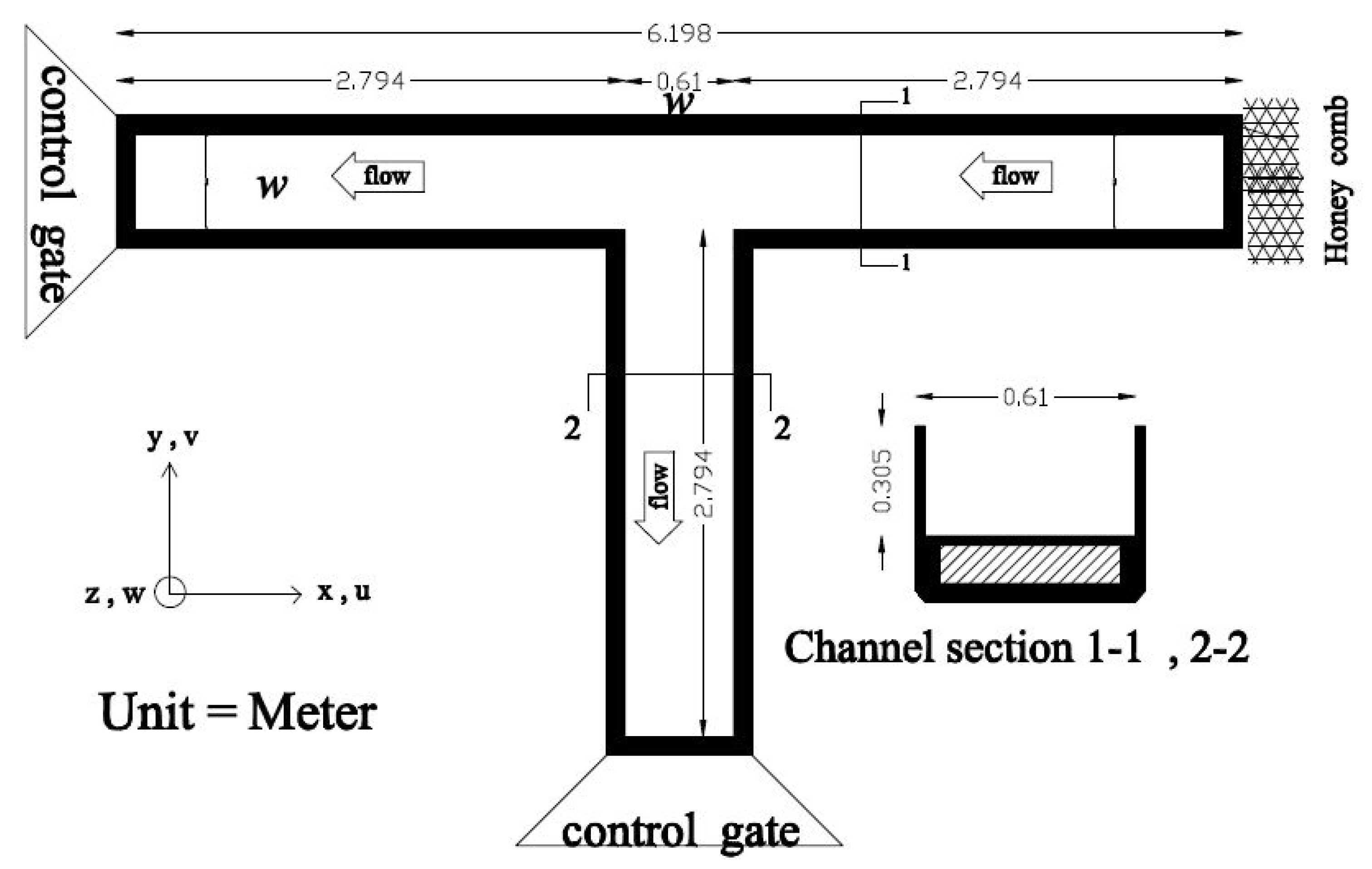
2.1. Experimental Model

Ramamurthy et al. [25] conducted their experiments in a horizontal channel with a 90-degree diversion, which directs the flow in the main and the branch channel illustrated in Figure 1 adapted from [25]. The length of the main channel is equal to 6.198 m and its branch is 2.794 m long. The widths of the channels are equal to 0.61 m and their heights are equal to 0.305 m. The branch channel is located 2.794 m away from the beginning of the main channel.
Taking into account that W*m is the width of the main channel and W*b is the width of the branch channel proposed by Ramamurthy et al. [25]. It has a width ratio of 1 (W*b/W*m = 1). The discharge entering the main channel entrance is equal to Qu = 0.046 m3/s. The discharge in the branch channel is equal to Qb = 0.038 m3/s. The branch channel discharge ratio to the main channel discharge (Qr = Qb/Qu) is equal to 0.838. All the parameters have been made dimensionless by the channel width (B = 0.61 m) and the main channel upstream critical velocity (Vc) in the experiments conducted by Ramamurthy et al. [25] and so the coordinate axes are defined in a dimensionless manner (x* = x/b’، y* = y/b, and z* = z/b). The dimensionless velocities in x, y, and z coordinates are marked as u*, v*, and w* respectively. The measurement locations in the channels according to an adaptation from Ramamurthy et al. [25] can be seen in Figure 2.

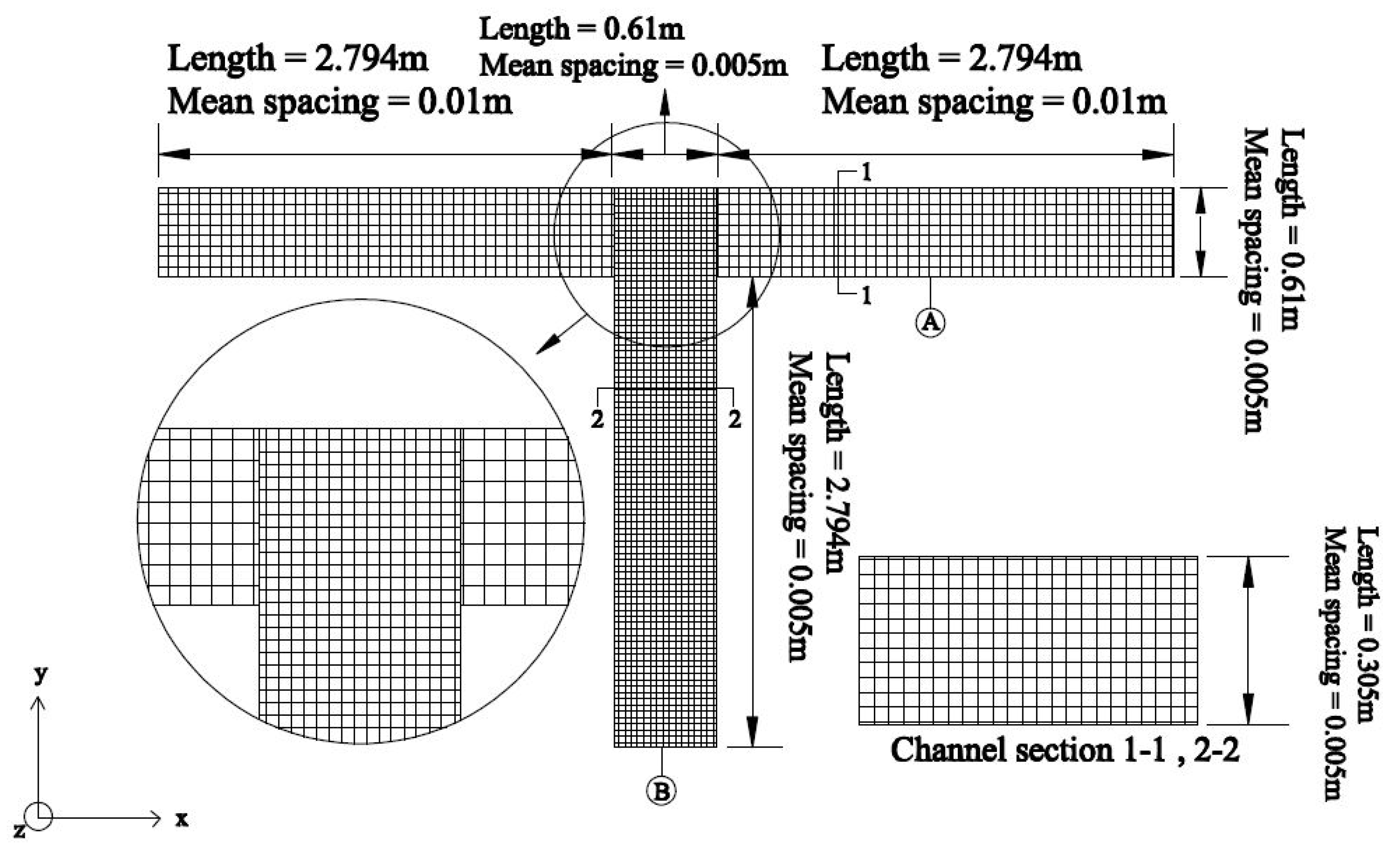
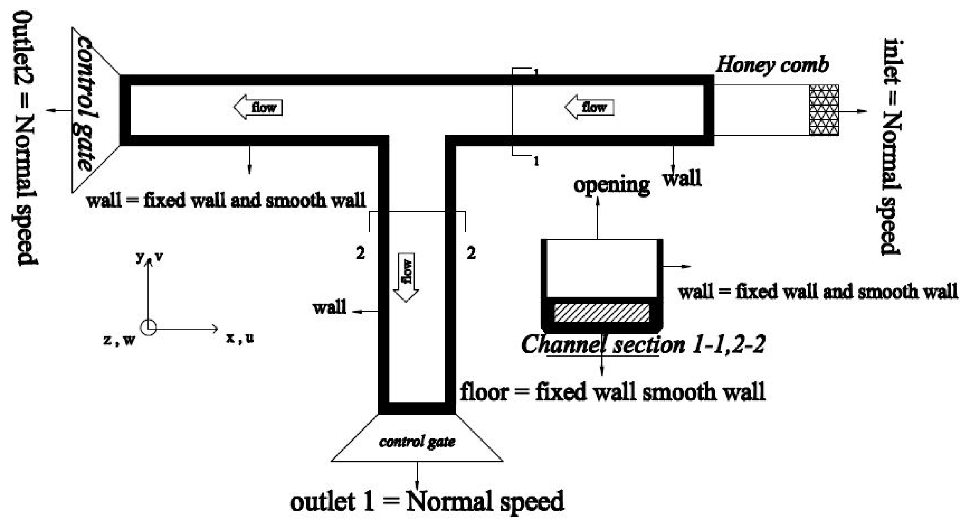
2.2. Simulating the Physical Model and the Flow Field

The CFD software aims at solving equations that describe a flow phenomenon. These equations include energy, mass, and motion force equilibrium. It solves the complete incompressible Reynolds-averaged Navier–Stokes through utilizing the finite-volume method in ANSYS-CFX software. It also uses powerful algorithms and discretization methods for solving the equations governing fluids and presents valid solutions [11,12]. Most of the flows occur in fact at high Reynolds levels, the experimental results indicate that the Reynolds number is between 15,000 and 30,000 in diversion flows. We therefore need to define an appropriate turbulence model to have accurate numerical answers. The three dimensional Reynolds time-averaged Navier–Stokes momentum equation for steady circumstances, and an incompressible turbulent flow continuity equation, have been used to solve the flow field problem in incompressible fluid:
A critical parameter among those in speeding up the execution of the model is the regional suitable reticulation in which the current flows in. To obtain an optimum reticulation in this modeling, we have divided the main channel into three sections. Its first section is 2.794 m in length which is located in the upstream of the main channel, its second section is 0.61 m long and is in the middle of the main channel, and its third section is 2.794 m long and is located in the downstream of the main channel. The size of the cells of the upstream and the downstream of the main channel is 1.0 cm × 0.5 cm × 0.5 cm, in the middle section it is 0.5 cm × 0.5 cm × 0.5 cm and the cells’ size of the branch channel network was selected to be 0.5 cm × 0.5 cm × 0.5 cm and the calculations were carried out using these sizes. The numerical obtained outcomes were compared with the experimental results and they resulted in an acceptable degree of consistency concerning the resulting error percentage and the calculations were carried out for 155,841 cells. Figure 3 indicates the plan and the façade of the calculative field reticulation in the intake with 90 degrees temperature.
In common flows with free surfaces, like that of the present study, the flow is a two-phase flow in which the air phase has been separated from the bottom phase, which is the water phase, by the free surface. One continuity equation is applied to each phase and the momentum equation has been separated for both phases and is solved commonly. The VOF two-phase method has been used in this research to solve the air–water two-phase field to specify the changes of the water surface within the field [25,26,27,28]. The boundary condition applied to the numerical model has been selected in such a manner that it will be consistent with the physical conditions of the experimental model of Ramamurthy et al. [25]. The boundary condition of normal velocity has been used in the entrance of the main channel and for the exit boundaries of the field (basin’s exit and the main channel) in this paper (Figure 4). The boundary conditions of the wall and the floor of the channel wall are assumed to be smooth and the walls being motionless and are used for a high level of opening boundary condition. Defining and determining the free surface of the flow field is determined according to the Eulerian viewpoint [11,12].

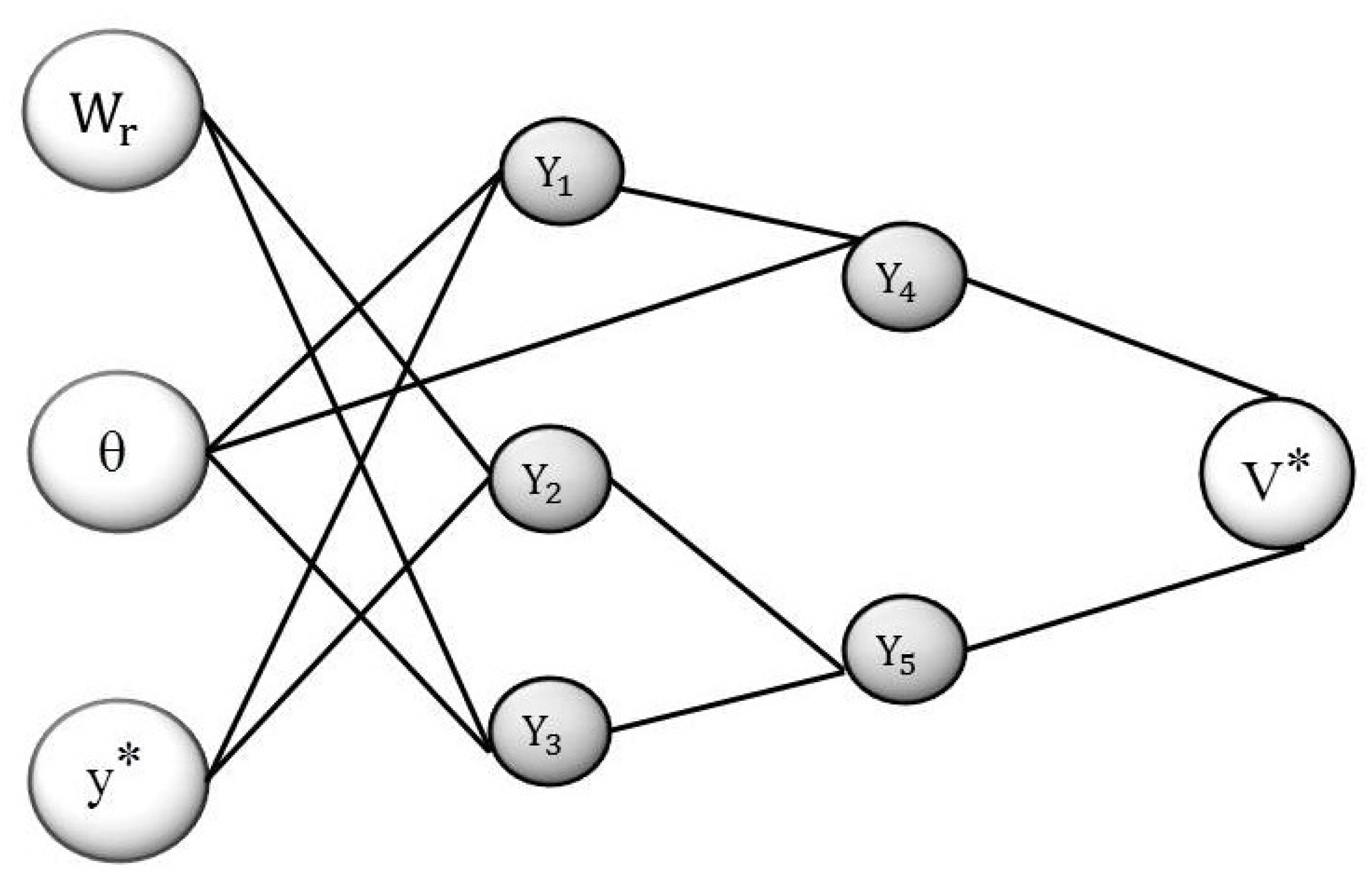
2.3. Overview of GMDH

Group method of data handling (GMDH) contains a set of neurons created by linking different pairs through a second-degree polynomial. The neural network combines the second-degree polynomials obtained from all the neurons and describes an approximate f ^ function with an y ^ output for a set of X = ( x 1 , x 2 , x 3 , , x n ) inputs with the minimum error in comparison with the real output, y. The actual results for M experimental data with n inputs and one output is therefore shown as Equation (1) [21,26,27,29,30]:
y i = f ( x i 1 , x i 2 , x i 3 , x i n )                                                 ( i = 1 , 2 , 3 , , M )
We aim to obtain a network which could predict the value of y ^ output for each X input axis based on the Equation (2):
y ^ i = f ^ ( x i 1 , x i 2 , x i 3 , x i n )                                                 ( i = 1 , 2 , 3 , , M )
It must also minimize the error of the predicted and actual values as shown below in addition to predicting the above equation:
M S E = 1 M i = 1 M ( y ^ i y i ) 2 M i n
The general form of the link between the input and output variables can be presented as below through utilizing a polynomial function,
y = a 0 + i = 1 n a i x i + i = 1 n j = 1 n a i j x i x j + i = 1 n j = 1 n k = 1 n a i j k x i x j x k +
The second degree of the above-mentioned equations, which will be used in this research, can be written as below [21,27,29,30]:
y ^ = G ( x i , x j ) = a 0 + a 1 x i + a 2 x j + a 3 x i 2 + a 4 x j 2 + a 5 x i x j
The ai unknown coefficients are obtained by regression methods in such a manner which the differences between the real output ‘y’ and the calculated ‘ y ^ ’ values are minimized for each pair of input variable xi and xj. A set of polynomials is made by considering the above-mentioned equation and all their unknown coefficients are obtained through considering the least square approach [21,27,29,30]. The coefficients of the equations of each neuron for minimizing its total error, to efficiently match the inputs with all the pairs of input–output sets, are obtained for each Gi function (each generated neuron).
E = 1 M i = 1 M ( y i G i ) 2 M i n
In primary methods of GMDH, all paired combinations (neurons) are generated from the input and the unknown coefficients of all neurons are obtained by using the least square. Therefore ( n 2 ) = n ( n 1 ) 2 neurons are generated in the second layer which could be expressed as shown below [21,29,30]:
{ ( y i , x i p , x i q ) | ( i = 1 , 2 , , M ) &     p , q q ( 1 , 2 , , M ) }
We will use the second degree of the function in Equation (5) for all M columns of three. The equations could be expressed in a matrix as follows [29,30]:
A a = Y
where A is the axis of the unknown coefficients of the second-degree equation indicated in Equation (5), meaning:
a = { a 0 , a 1 , , a 5 }
Y = { y 1 , y 2 , y 3 , , y M }
A = [ 1             x 1 p                 x 1 p 2                 x 1 q 2                   x 1 p x 1 q 1             x 2 p               x 2 p 2                 x 2 q 2                   x 2 p x 2 q                                                                                             1             x M p             x M p 2             x M q 2               x M p x M q ]
The method of least squares analysis of multiple-regression solves the equations as follows [21,29,30]:
a = ( A T A ) 1 A T Y )
This equation creates all the coefficients of Equation (10) for all the M triple sets [21,29,30].

3. Results and Discussion

Following that, a GMDH model will be introduced for 30-, 60-, and 90-degree diversion angles and 1.4, 1.2, 1.0, 0.8, and 0.6 width ratios to forecast the mean velocity of the stream. It is essential to model and verify a numerical model to train the model under conditions where there are no experimental results; therefore, Ramamurthy et al.’s [25] experimental model was simulated through using the ANSYS-CFX software. This model is then verified using the existing experimental data. After making sure that the CFX has simulated the model accurately, different models were run by using CFX and used to train and verify GMDH to forecast the mean velocity of the stream. Following that and after making sure that GMDH performs well, the mean velocity is predicted for the width ratios and angles on which there is no experimental model. For the model is based on the criteria of the coefficient of determination (R2), root mean square error (RMSE), mean absolute percentage error (MAPE) and SI as defined in the following forms:
R 2 = [ i = 1 n ( x i n   x ¯ ) ( y i n y ¯ ) / i = 1 n ( x i n x ¯ ) 2 i = 1 n ( y i n y ¯ ) 2 ] 2
R M S E = 1 n i = 1 n ( x i n y i ) 2
M A P E = 1 n i = 1 n | x i n y i | x i
S I = R M S E x ¯
where yi and xi are the calculated and real mean velocity values, respectively, and y ¯ and x ¯ are the mean calculated and real mean velocity values, respectively.

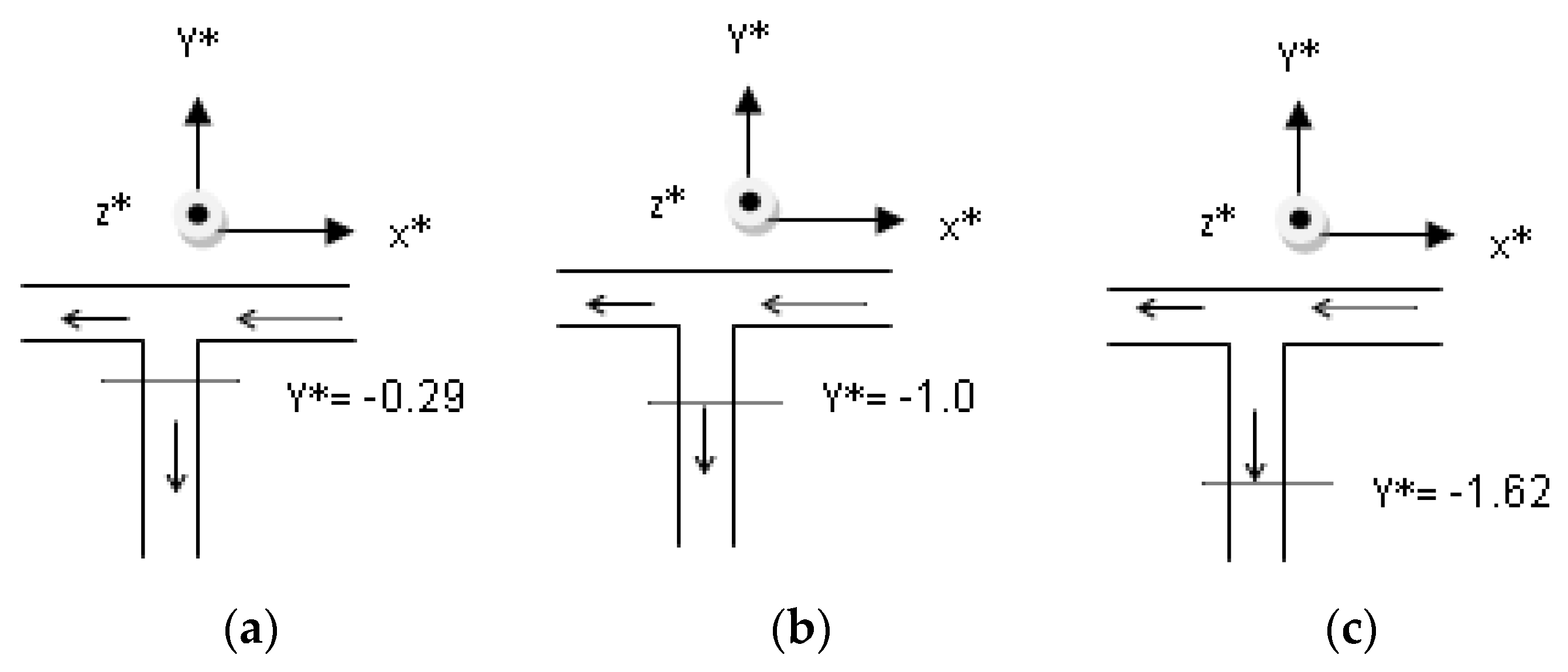
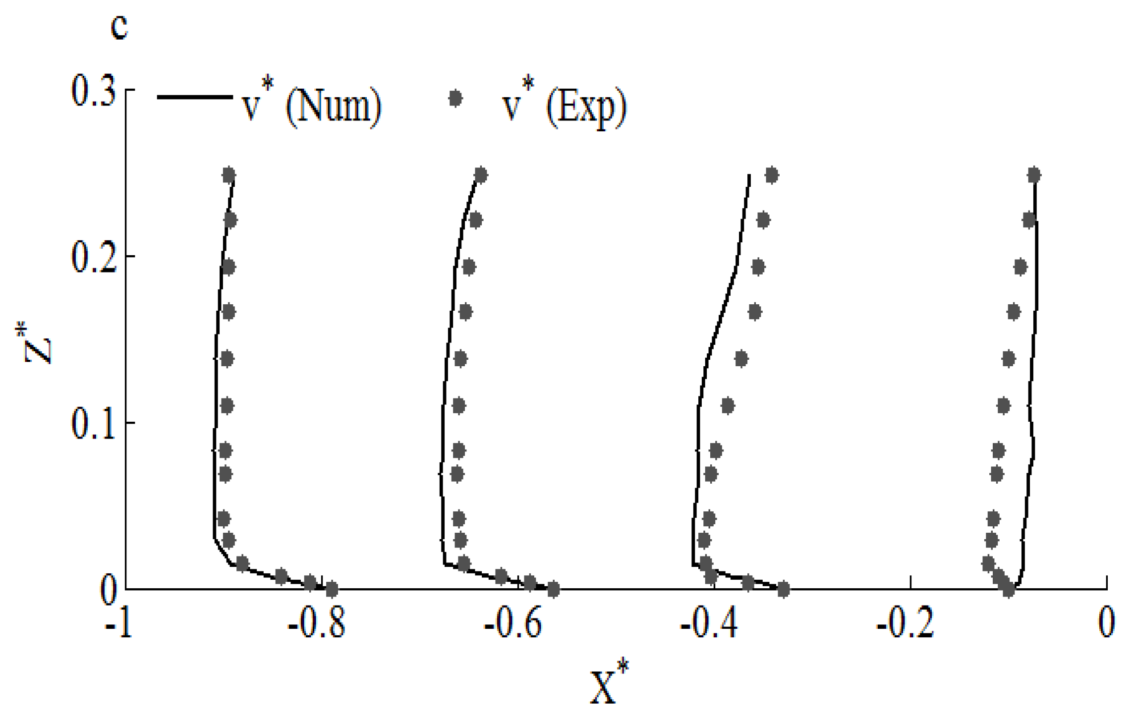
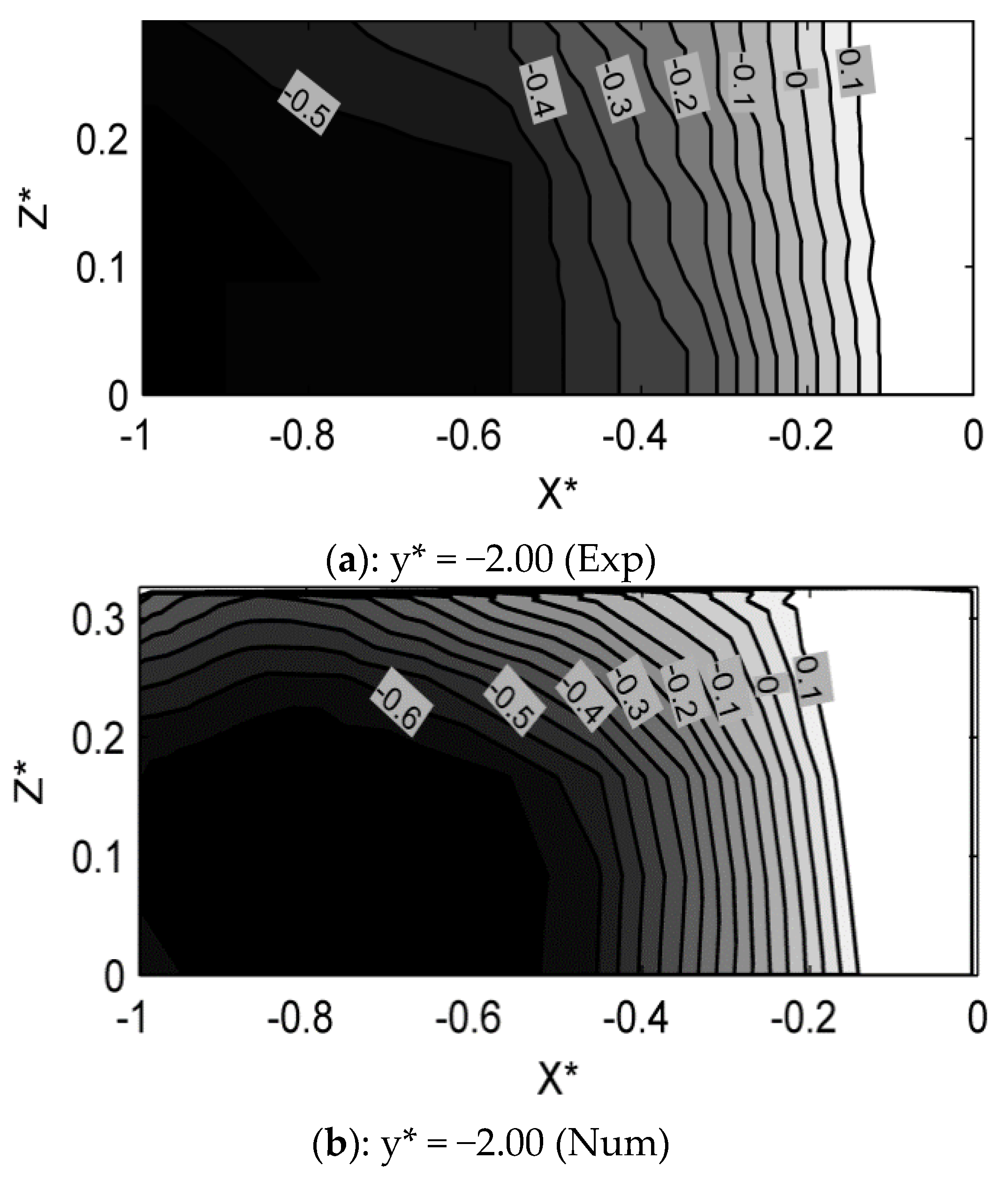
3.1. Verifying of CFX

The verification of the CFX model’s results has been evaluated in three y* = 1.62, −1.0, and −0.29 cross-sections of the branch channel. Table 1 shows the statistical indexes for comparing the numerical model’s results and the experimental model’s results in different y* cross-sections.
The mean relative error MAPE has been obtained to be 5% in this comparison therefore Figure 5 shows a good consistency existing between the results of the CFX model and the outcomes of the experimental model. In three cross-sections y* = −1.62, −1.0, and −0.29, the mean relative error MAPE has been obtained to be approximately 2%, 5.2%, and 6.95%, respectively, concerning Table 1. The value of RMSE is equal to 0.012, 0.01, and 0.017 for cross-section y* = −1.62, −1.0, and −0.29, respectively, and the amount of R2 for three y* = −1.62, −1.0, and −0.29 cross-section is 0.88, 0.68, and 0.95, respectively, in the table. In y* = −1.0 and y* = −1.62 in the branch channel downstream, the values of the longitudinal velocity increase in the direction against the flow and the velocities become negative due to the presence of the recirculation zone in the separation zone. In depths of z* = 0.0 to z* = 0.2 and in the contraction zone the velocities are maximum Vmax and the contraction zone is denser than the flow surface in this area since the flow lines are denser. The amount of SI for three y* = −1.62, −1.0, and −0.29 cross-section is 0.025, 0.061, and 0.082, respectively.
The profiles of the flow longitudinal velocity in y* = −2.00 cross section of the branch channel were drawn in 0.838 discharge in the numerical model and the experimental model was drawn to examine the matter more carefully (Figure 6). Contours (a) and (b) present the longitudinal velocities of the flow in the generated experimental model and numerical model respectively in Figure 5 Concerning the Figure 6, the values of the longitudinal velocity increase along the opposite direction of the stream and cause severe fluctuations in the stream longitudinal velocity in y* = −2.00 since the recirculation zone has completely developed in the separation zone. Concerning the figure, the longitudinal velocities reach the maximum value Vmax in x* = 0.4 to x* = 0.7 area and in the depth of z* = 0.0 to z*0.2 and so the intensity of the velocity fluctuation is greater in this area in comparison with the flow surface and the other areas of the intake channel.

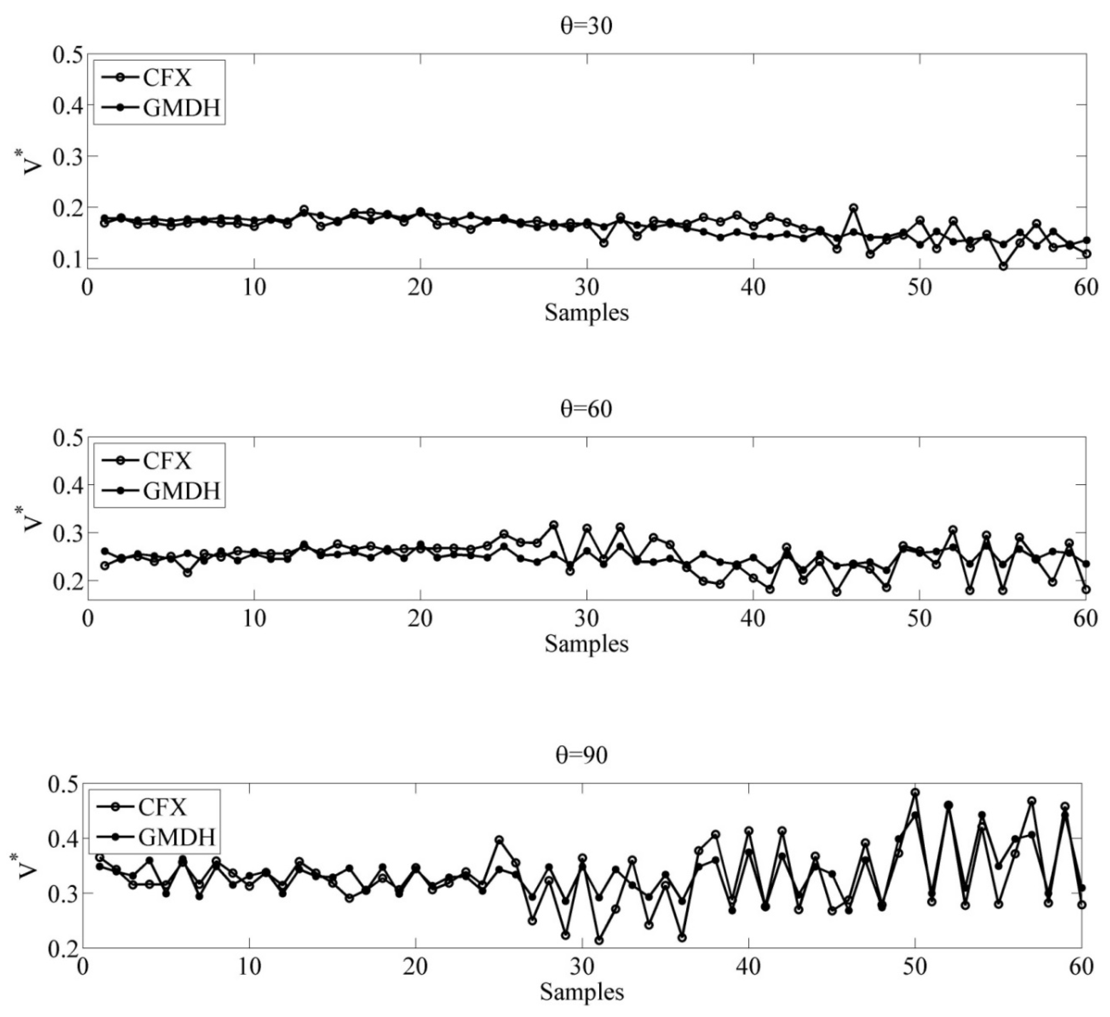
3.2. Derivation of Mean Velocity using GMDH

GMDH is used in the present research to present an equation for predicting the relative velocity in the branch channel (V*) in an intake. The independent parameters influencing the prediction of the dependent variable, V*, include the ratio of the branch channel width to the main channel (Wr), diversion angle with the longitudinal direction of the main channel (θ), and the longitudinal coordinates in the intake channel (y*) which are introduced as below:
V * = f ( W r , θ , y * )
The data obtained from the numerical simulation by CFX need to be divided into two groups of training and testing to predict V* therefore we could examine the flexibility of the model for different data. Therefore, 30% of data (180 data) are CROSS-VALIDATION selected from amongst the 600 existing data and the rest 70% (420 data) are utilized to train the model. Figure 7 shows the evolved structure of generalized GMDH neural network for modeling the relative velocity in the branch channel. Moreover, the equations obtained through using GMDH for modeling V* are presented as below:
Y 1 = 0.0719 + 0.234 θ + 0.0281 y * 0.0206 θ 2 + 0.0175 y * 2 + 0.0347 θ × y *
Y 2 = 0.178 + 0.242 W r + 0.0279 y * 0.122 W r 2 + 0.0175 y * 2 + 0.0405 W r × y *
Y 3 = 0.0314 + 0.162 W r + 0.166 θ 0.122 W r 2 0.0205 θ 2 + 0.0284 W r × θ
Y 4 = 0.142 0.549 θ + 4.43 Y 1 0.466 θ 2 19.865 Y 1 2 + 6.173 θ × Y 1
Y 5 = 0.2822 1.6592 Y 2 0.4352 Y 3 + 1.593 Y 2 2 0.579 Y 3 2 + 6.917 Y 2 × Y 3
V * = 0.011 1.772 Y 4 + 2.666 Y 5 + 22.136 Y 4 2 + 13.628 Y 5 2 35.634 Y 4 × Y 5
Figure 8 indicates the performance of the model presented by using GMDH for the purposes of predicting the mean velocity for different angles including the 30-, 60-, and 90-degree angles. The predictions made at θ = 30 is almost very well consistent with the values obtained from CFX in most of the points. In points where the values estimated by the GMDH are different from the target values (the values obtained from CFX), the predictions do not follow a particular pattern and both overestimate and underestimate the values of these differences are however not significant with regard to the Figure 7. The relative velocities obtained in this angle have mostly values smaller than 0.2 m/s. As θ increases, the values of the relative velocities also decrease in accordance with the Figure. In such a manner that at θ = 60, the relative velocity is smaller than 0.3 m/s and at θ = 90 it is lesser than 0.4 m/s. As θ increases the accuracy of the predictions relatively decreases; however, it could not be specified at which exact angle it performs best; therefore, the accuracy of the predictions are examined quantitatively through using Table 1 and Figure 8. In the values (θ = 30-, 60-, and 90-degree, samples 25–45), eddy and rotational currents are more and the direction of flow velocity changes, and the measurement error is more likely in these values. Therefore, the results presented by ANSYS-CFX numerical software and GMDH method in areas where secondary currents and vortices are more intense, have more differences and higher error rates.
Table 2 shows the results obtained from the model presented for the purposes of forecasting the mean velocity through the use of different statistical indexes for different width ratios at 30-, 60-, and 90-degree angles. In the training mode of the model at 0.6 width ratio, the maximum relative error is related to θ = 60 which is equal to 6.8% although similar results could also be seen for the other two angles. Therefore, the presented model shows good results for different angles at 0.6 width ratio. As the width ratio increases and at Wr = 0.8 the prediction accuracy decreases in such a manner that the maximum relative error is approximately 8% which occurs at θ = 30 while it presents almost similar results to that of the existing width ratio at the two other θs. Greater increase in the width ratio value decreases the prediction accuracy but the outstanding point is that the total mean of all the predictions made in this research in the training mode of the model is as R2 = 0.86, MAPE = 10.44, RMSE = 0.03, and SI = 0.12, which shows that the model is fairly accurate for all the training data.
The results of the statistical indexes in the testing mode of the model are almost similar to those of the training mode of the model. In such a manner that at 6% width ratio the relevant maximum relative error is approximately 6% which also follows an almost similar process at 0.8 width ratio. Like the training mode, as the width ratio increases the prediction accuracy decreases in this mode as well, however, what stands up in this table is that the velocity prediction results at the test mode of the model (R2 = 0.88, MAPE = 9.72, RMSE = 0.03, and SI = 0.11) also follow an almost similar process to that of the training mode of the model which indicates the flexibility of the presented model under different hydraulic conditions.
Figure 9 shows the error distribution of the presented model for different width ratios (Figure 9b) and different angles (Figure 9a). In statistics, a frequency distribution is a graph that displays the frequency of various outcomes in a sample. Each entry in the table contains the frequency or count of the occurrences of values within a particular group or interval. It could be seen that the relative error distribution is almost constant in all three models at different angles. The point to be considered in this Figure 9 is that almost 80% of the data used in this study have a relative error less than 15% which indicates that the model presented in the present study through using GMDH performs well when determining the mean velocity. It could also be seen at different width ratios that the predictions made have a relative error less than 10% at the width ratio of approximately 90%. The maximum error values are related to 1.4 width ratio but as seen almost 70% of the predictions have a relative error less than 15% in this state as well which reveals that the model suggested in the current research performs well.
It could be stated in general and with regard to Figure 8 and Figure 9 which show the differences between the estimated values and the real values and the relative error distribution respectively and also the values of the statistical indexes presented in Table 2, which have presented relatively good results for different angles and width ratios, that using the equation which has been presented in this study can perform well in predicting the mean velocity in an intake (Equation (23)) and it could decrease the problems stemming from experimental researches which are usually time- consuming and costly, with a relatively fair level of accuracy.

4. Conclusions

Numerical analysis and group method of data handling is used in the present study to present an equation for estimating the mean velocity (V*) in open channel intakes. The diversion angle with the longitudinal direction of the main channel (θ), the longitudinal coordinates in the intake channel (y*), and the ratio of branch channel width to the main channel (Wr), and experimental data dimensionless parameters were utilized to predict this parameter. The experimental model presented by Ramamurthy et al. [25] has been first numerically simulated by using ANSYS-CFX. Different simulations were then carried out with regard to the numerical model’s ability to simulate the flow field at 30- and 60-degree intake angles and different ratios of branch channel width to the main channel. The results were used to present an equation for the purposes of predicting the main velocity. The results of the carried out verifications, (MAPE (mean) = 5% and RMSE (max) = 0.017, R2 = 0.95, SI = 0.025), indicated that the simulation was fairly accurate. Therefore, with regard to the fact that the numerical model performed fairly accurately in simulating the experimental conditions, the numerical model’s data were used to present a model by using GMDH to estimate the mean velocity. The results of the statistical indexes used to quantitatively examine this model, (R2 = 0.86, MAPE = 10.44, RMSE = 0.03, and SI = 0.12), indicated the accuracy of this model in predicting the mean velocity of the flow within open channel intakes. Like the training mode, as the width ratio increases the prediction accuracy decreases. The velocity prediction results at the model’s test mode (R2 = 0.88, MAPE = 9.72, RMSE = 0.03, and SI = 0.11) also follow a similar trend to training mode of the model which indicates the flexibility of the presented model under different hydraulic conditions. It is, therefore, advisable to use the model presented in this study (Equation (23)), which is reasonably accurate. It could also be seen at different width ratios that the predictions made have a relative error of less than 10% at the width ratio of approximately 90%. The maximum error values are related to a 1.4 width ratio. It is worth mentioning that almost 70% of the predictions have a relative error less than 15% in this state, which reveals that the proposed model performs with high performance. Although the manuscript brings significant novelty in predicting velocity in channel intake through a hybridized CFD model, other data-driven methods’ applicability is yet to be explored. Future research can immensely benefit from the involvement of advanced machine learning and deep learning techniques hybridized by the CFD codes.

Author Contributions

Data curation, S.S.B., I.A.-S., H.K., S.K., J.E., and A.M.; formal analysis, S.S.B., I.A.-S., H.K., S.K., J.E., and A.M.; investigation, S.S.B., I.A.-S., H.K., S.K., J.E., and A.M.; project administration, S.S.B., I.A.-S., H.K., S.K., J.E., and A.M.; software, S.S.B., I.A.-S., H.K., S.K., J.E., and A.M.; supervision, S.S.B. and A.M.; validation, H.K.; visualization, S.S.B., I.A.-S., H.K., S.K., J.E., and A.M.; writing—original draft, H.K.; writing—review and editing, S.S.B., I.A.-S., H.K., S.K., J.E., and A.M. All authors have read and agreed to the published version of the manuscript.

Funding

This research in part is supported by the Hungarian State and the European Union under the EFOP3.6.2-16-2017-00016 project.

Acknowledgments

Support of the Alexander von Humboldt Foundation is acknowledged.

Conflicts of Interest

The authors declare that there is no conflict of interests regarding the publication of this paper.

References

  1. Grace, J.L.; Priest, M.S. Division of Flow in Open Channel Junctions; Engineering Experiment Station, Alabama Polytechnic Institute, Auburn University: Auburn, AL, USA, 1958. [Google Scholar]
  2. Neary, V.S.; Odgaard, A.; Sotiropoulos, F. Three-dimensional numerical model of lateral-intake inflows. J. Hydraul. Eng. 1999, 125, 126–140. [Google Scholar] [CrossRef]
  3. Hager, W.H. Discussion of separation zone at Open-Channel Junctions. by James L. Best and Ian Reid. J. Hydraul. Eng. 1987, 113, 539–543. [Google Scholar] [CrossRef]
  4. Karimi, S.; Bonakdari, H.; Gholami, A. Determination Discharge Capacity of Triangular Labyrinth Side Weir using Multi-Layer Neural Network (ANN-MLP), Special Issue of Current World Environment 10 (Special Issue May 2015). 2015. Available online: http://www.cwejournal.org/?p=10430:111-119 (accessed on 3 August 2020).
  5. Law, S.W.; Reynolds, A.J. Dividing flow in an open channel. J. Hydraul. Div. 1966, 92, 4730–4736. [Google Scholar]
  6. Neary, V.S.; Odgaard, A.J. Three-dimensional flow structure at open channel diversions. J. Hydraul. Eng. 1993, 119, 1224–1230. [Google Scholar] [CrossRef]
  7. Karimi, S.; Bonakdari, H.; Ebtehaj, I.; Zaji, A.H. Prediction of Mean Velocity in Open Channel Intake Using Numerical Model and Gene Expression Programming. Mitt. Saechsischer Entomol. (MSE) 2016, 119, 599–616. [Google Scholar]
  8. Kasthuri, B.; Pundarikanthan, N.V. Discussion of “separation zone at open channel junction”. J. Hydraul. Eng. 1987, 113, 543–544. [Google Scholar] [CrossRef]
  9. Weber, L.J.; Schumate, E.D.; Mawer, N. Experiments on flow at a 90 open-channel junction. J. Hydraul. Eng. 2001, 127, 340–350. [Google Scholar] [CrossRef]
  10. Shamloo, H.; Pirzadeh, B. Numerical investigation of velocity field in dividing open-channel flow. In Proceedings of the 12th WSEAS International Conference on APPLIED MATHEMATICS 194–199, Cairo, Egypt, 29–31 December 2007. [Google Scholar]
  11. Bonakdari, H.; Baghalian, S.; Nazari, F.; Fazli, M. Numerical analysis and prediction of the velocity field in curved open channel using Artificial Neural Network and Genetic Algorithm. Eng. Appl. Comput. Fluid Mech. 2011, 5, 384–396. [Google Scholar] [CrossRef]
  12. Baghalian, S.; Bonakdari, H.; Nazari, F.; Fazli, M. Closed-form solution for flow field in curved channels in comparison with experimental and numerical analyses and Artificial Neural Network. Eng. Appl. Comput. Fluid Mec. 2012, 6, 514–526. [Google Scholar] [CrossRef]
  13. Mohamad, E.T.; Faradonbeh, R.S.; Armaghani, D.J.; Monjezi, M.; Abd Majid, M.Z. An optimized ANN model based on genetic algorithm for predicting ripping production. Neural Comput. Appl. 2017, 28, 393–406. [Google Scholar] [CrossRef]
  14. Shiri, J.; Dierickx, W.; Neamati, A.; Ghorbani, M.A. Estimating daily pan evaporation from climatic data of the State of Illinois, USA using adaptive neuro-fuzzy inference system (ANFIS) and artificial neural network (ANN). Hydrol. Res. 2011, 42, 491–502. [Google Scholar] [CrossRef]
  15. Ebtehaj, I.; Bonakdari, H. Performance Evaluation of Adaptive Neural Fuzzy Inference System for Sediment Transport in Sewers. Water Resour. Manag. 2014, 28, 4765–4779. [Google Scholar] [CrossRef]
  16. Ebtehaj, I.; Bonakdari, H. Bed load sediment transport estimation in a clean pipe using multilayer perceptron with different training algorithms. KSCE J. Civ. Eng. 2016, 20, 581–589. [Google Scholar] [CrossRef]
  17. Bonakdari, H.; Ebtehaj, I. Comparison of two data-driven approaches in estimation of sediment transport in sewer pipe. In Proceedings of the 36th IAHR World Congress, The Hague, The Netherlands, 28 June–3 July 2015. [Google Scholar]
  18. Ebtehaj, I.; Bonakdari, H. Comparison of genetic algorithm and imperialist competitive algorithms in predicting bed load transport in clean pipe. Water Sci. Technol. 2014, 70, 1695–1701. [Google Scholar] [CrossRef] [PubMed]
  19. Basser, H.; Karami, H.; Shamshirband, S.; Akib, S.; Amirmojahedi, M.; Ahmad, R. Hybrid ANFIS–PSO approach for predicting optimum parameters of a protective spur dike. Appl. Soft Comput. 2015, 30, 642–649. [Google Scholar] [CrossRef]
  20. Najafzadeh, M.; Barani, G.H.A.; Azamathulla, H.M.D. GMDH to Predict Scour Depth around Vertical Piers in Cohesive Soils. Appl. Ocean Res. 2013, 40, 35–41. [Google Scholar] [CrossRef]
  21. Akbarizadeh, M.; Daghbandan, A.; Yaghoob, Y.I. Modeling and Optimization of Poly Electrolyte Dosage in Water Treatment Process by GMDH Type-NN and MOGA. Int. J. Chemoinformatics Chem. Eng. (IJCCE) 2013, 3, 94–106. [Google Scholar] [CrossRef] [Green Version]
  22. Sheikholeslami, M.; Sheykholeslami, F.B.; Khoshhal, S.; Mola-Abasia, H.; Ganji, D.D.; Rokni, H.B. Effect of magnetic field on Cu–water nanofluid heat transfer using GMDH-type neural network. Neural Comput. Appl. 2014, 25, 171–178. [Google Scholar] [CrossRef]
  23. Atashrouz, S.; Pazuki, G.; Alimoradi, Y. Estimation of the viscosity of nine nanofluids using a hybrid GMDH-type neural network system. Fluid Phase Equilibria 2014, 372, 43–48. [Google Scholar] [CrossRef]
  24. Ayoub, M.A.; Negash, B.M.; Saaid, I.M. Modeling Pressure Drop in Vertical Wells Using Group Method of Data Handling (GMDH) Approach; Springer: Singapore, 2015; pp. 69–78. [Google Scholar]
  25. Ramamurthy, A.; Qu, J.; Vo, D. Numerical and experimental study of dividing open-channel flows. J. Hydraul. Eng. 2007, 133, 1135–1144. [Google Scholar] [CrossRef]
  26. Mignot, E.; Bonakdari, H.; Knothe, P.; LipemeKouyi, G.; Bessette, A.; Rivière, N.; Bertrand-Krajewski, J.L. Experiments and 3D simulations of flow structures in junctions and their influence on location of flowmeters. Water Sci. Technol. 2012, 66, 1325–1332. [Google Scholar] [CrossRef] [PubMed]
  27. Najafzadeh, M.; Lim, S.Y. Application of improved neuro-fuzzy GMDH to predict scour depth at sluice gates. Earth Sci. Inf. 2015, 8, 187–196. [Google Scholar] [CrossRef]
  28. Wilcox, D.C. Turbulence Modeling for CFD, 2nd ed.; Industries, Inc: La Canada Flintridge, CA, USA, 2000. [Google Scholar]
  29. Ebtehaj, I.; Bonakdari, H.; Khoshbin, F.; Azimi, H. Pareto genetic design of group method of data handling type neural network for prediction discharge coefficient in rectangular side orifices. Flow Meas. Instrum. 2015, 41, 67–74. [Google Scholar] [CrossRef]
  30. Bagheri-Esfe, H.; Safikhani, H. Modeling of deviation angle and performance losses in wet steam turbines using GMDH-type neural networks. Neural Comput. Appl. 2017, 28, 489–501. [Google Scholar] [CrossRef]
Figure 1. The plan of the experimental channel used in current research.
Applsci 10 07521 g001
Figure 2. The measurement locations (a): Y* = −0.29, (b): Y* = −1.00 and (c): Y* = −1.62 in the channels.
Applsci 10 07521 g002
Figure 3. Gridding the plan and the cross-section of the simulated model using the ANSYS-CFX.
Applsci 10 07521 g003
Figure 4. Boundary condition of the simulated model using the ANSYS-CFX.
Applsci 10 07521 g004
Figure 5. Verification graphs between the results of the CFX model and the Ramamurthy and his colleagues’ experimental model in: (a) y* = −0.29, (b) y* = −1.00, and (c) y* = −1.62.
Applsci 10 07521 g005aApplsci 10 07521 g005b
Figure 6. Verification graphs between the outcomes of the CFX model and the Ramamurthy and his colleagues’ experimental model in y* = −2.00.
Applsci 10 07521 g006
Figure 7. Evolved structure of generalized group method of data handling (GMDH) neural network for modeling and prediction of mean velocity.
Applsci 10 07521 g007
Figure 8. Performance of outcomes for testing phase of the GMDH model at different angles.
Applsci 10 07521 g008
Figure 9. Error distribution of GMDH for (a) different angle (θ) (b) different relative width of branch channel to main channel (Wb*/Wm*).
Applsci 10 07521 g009
Table 1. Statistical index for the verification outcomes of the numerical model.
y* = −0.29y* = −1.0y* = −1.62
RMSE0.010.0120.017
MAPE (%)2.05.26.95
R20.950.880.68
SI0.0250.0610.082
Table 2. Performance evaluation of presented model by GMDH for training and testing stage.
TrainWrθR2MAPERMSESI
0.6300.504.350.010.05
600.606.800.020.08
900.485.720.020.07
0.8300.548.310.020.11
600.245.240.020.06
900.594.940.020.07
1.0300.438.790.020.10
600.8510.630.040.14
900.7316.570.050.17
1.2300.6513.940.030.18
600.6016.040.040.17
900.859.960.040.11
1.4300.2418.580.030.23
600.6616.860.040.17
900.909.840.040.11
All 0.8610.440.030.12
Test0.6300.544.180.010.05
600.575.780.020.07
900.604.840.020.06
0.8300.295.400.010.07
600.105.100.020.06
900.484.070.020.06
1.0300.336.510.010.08
600.8010.420.040.13
900.8117.510.050.17
1.2300.5915.660.030.17
600.5714.600.030.16
900.878.690.030.10
1.4300.1919.980.030.23
600.8514.420.040.15
900.938.630.040.10
All 0.889.720.030.11
Publisher’s Note: MDPI stays neutral with regard to jurisdictional claims in published maps and institutional affiliations.

