Deep Learning-Based Portable Device for Audio Distress Signal Recognition in Urban Areas

Abstract

Real-time automatic identification of audio distress signals in urban areas is a task that in a smart city can improve response times in emergency alert systems. The main challenge in this problem lies in finding a model that is able to accurately recognize these type of signals in the presence of background noise and allows for real-time processing. In this paper, we present the design of a portable and low-cost device for accurate audio distress signal recognition in real urban scenarios based on deep learning models. As real audio distress recordings in urban areas have not been collected and made publicly available so far, we first constructed a database where audios were recorded in urban areas using a low-cost microphone. Using this database, we trained a deep multi-headed 2D convolutional neural network that processed temporal and frequency features to accurately recognize audio distress signals in noisy environments with a significant performance improvement to other methods from the literature. Then, we deployed and assessed the trained convolutional neural network model on a Raspberry Pi that, along with the low-cost microphone, constituted a device for accurate real-time audio recognition. Source code and database are publicly available.

Dataset:https://github.com/jfgf11/Problema-Especial.git

1. Introduction

The rapid growth of the urban population has led to an increased use of technology to improve quality of life, productivity, and to address environmental challenges. One of the many obstacles that big cities face is improving emergency systems which rely heavily on response times that may be affected by cities size and population. In criminology, the effectiveness of rapid response has been long questioned because police action becomes irrelevant if notification times are too slow [1]. According to NYC 911 reporting, in New York, the most populous city in the U.S., an average 911 call for critical emergencies takes approximately 3.59 min to be both processed by the call taker and the first responders dispatched. To alleviate this problem, technological solutions have been proposed to reduce the time it takes to answer and process an emergency call, particularly when the target scenario is in urban areas. These developments are mostly focused on detection via visual input rather than audio ones because, in public places, background noise is a concern and the detection of events that overlap with noise can be a challenging task. Moreover, the distance of the sound source to the microphone can make it difficult to detect certain events. Examples of machine learning surveillance systems based on visual input involve detecting abnormal behavior through action recognition which aims to distinguish activities such as violence identification [2], drowning identification [3], and atypical human falling detection [4].

Very little has been done to develop automatic systems for the recognition of audio distress signals in open urban areas. In this context, audio distress signals refer to emergency shouts coming from distressed people in the streets that can be either just a shout that contains no speech or a phrase in shouted form such as “help me!” The automatic detection of audio distress signals is a challenging task because these systems have to recognize both speech and emotion, and discriminate between a normal street sound, such as a salesman shouting offers in the street, and an actual emergency shout. Multiple databases that collect vocal distress signals have been constructed and tested using standard recognition models. For example, the database presented in [5] includes audios with utterances of emotional speech. Moreover, the databases presented in [6,7] include audios that are labeled with different types of emotions and recorded in low noise environments as houses or closed locations. The work in [8] presented a large database that includes screaming sounds that were artificially overlapped with white additive Gaussian noise. These databases have been useful to study the development of models for the automatic recognition of audio distress signals, and have been used to validate recognition models for sentiment analysis, as presented in [9,10,11,12]. Audios in these databases are typically recorded in low noise environments using expensive high-quality microphones, limiting the reach of real implementations.

In this paper, we propose a device implementation that locally uses deep convolutional neural networks to detect and classify different audio distress signals in real urban areas. Such devices can potentially improve response times in emergency alert systems in smart cities. Our contribution to this subject is twofold: (i) a device that is designed to accurately conduct the recognition task in urban areas where generally loud noise is a concern, and (ii) a device that is portable and low cost. To design such device, we first created a database with information from real scenarios to train the deep learning model (Section 2.2). Audios were recorded in real urban scenarios using an affordable microphone. Then, we developed a strategy to train a classifier based on temporal and frequency data analysis (Section 2.3) and deep convolutional neural networks (Section 2.4). Through experimental results, we show that the convolutional neural network model outperforms methods that have been previously used in audio distress signal recognition (Section 3). Finally, we deployed the trained neural network model on a Raspberry Pi and evaluated the computational performance of the real-time recognition system (Section 3.4). Currently, the Raspberry Pi represent a useful element to construct inexpensive portable devices that compute complex tasks in real time [13,14]. We end this paper with some conclusions and future work (Section 4). The collected dataset and the implemented scripts are publicly available at the github repository in the link above.

2. Materials and Methods

To construct the recognition model, we first collected a database in real urban scenarios. Then, we used two techniques to extract time and frequency information from audio signals in a given time window that was used as input data to convolutional neural networks to conduct the classification task. Following, we provide a detailed explanation of each one of these steps.

2.1. Prototype Design

The general design of the prototype is shown in Figure 1. It consists of a condenser microphone and a Raspberry Pi located at a two meter tall structure.

We used a Raspberry Pi 4 model B, which has a 64-bit quad-core processor and up to 4 GB of RAM. The source code was written in Python, containing a copy of the trained model of the convolutional neural network that was uploaded trough GitHub. The chosen audio sensing device is the Snowball iCE Condenser microphone. It is important to note that this is a low-cost device. The reach of this microphone is defined by the cardioid polar pattern shown in [15].

The total cost of implementation is around $150USD, which includes the microphone ($50USD), the Raspberry Pi device ($60USD), and additional elements such as a micro-sd card, case, and stand. Comparing this cost to the audio device used in [8], which is above $450USD dollars (high-quality microphone), our device can be considered as a low-cost one.

2.2. Database Collection

We collected audios in real urban scenarios using a low-cost microphone with the aim of developing an inexpensive device that works in a real-world scenario. First, we asked 100 people to propose expressions in Spanish language that they would scream in a situation where they required help in public spaces. The three most commonly suggested signals were the wordless shout “Ahhhhh”, “auxilio” (help), and “ayuda” (synonym of help). From now on, we will refer to those noises as SN (shout noise), HN (help noise), and AN (aid noise), respectively. Audio collection was conducted in multiple real urban environments with different signal-to-noise ratio values, where background levels were classified into 3 categories: low, medium, and high. The following procedure was conducted for the audio collection.

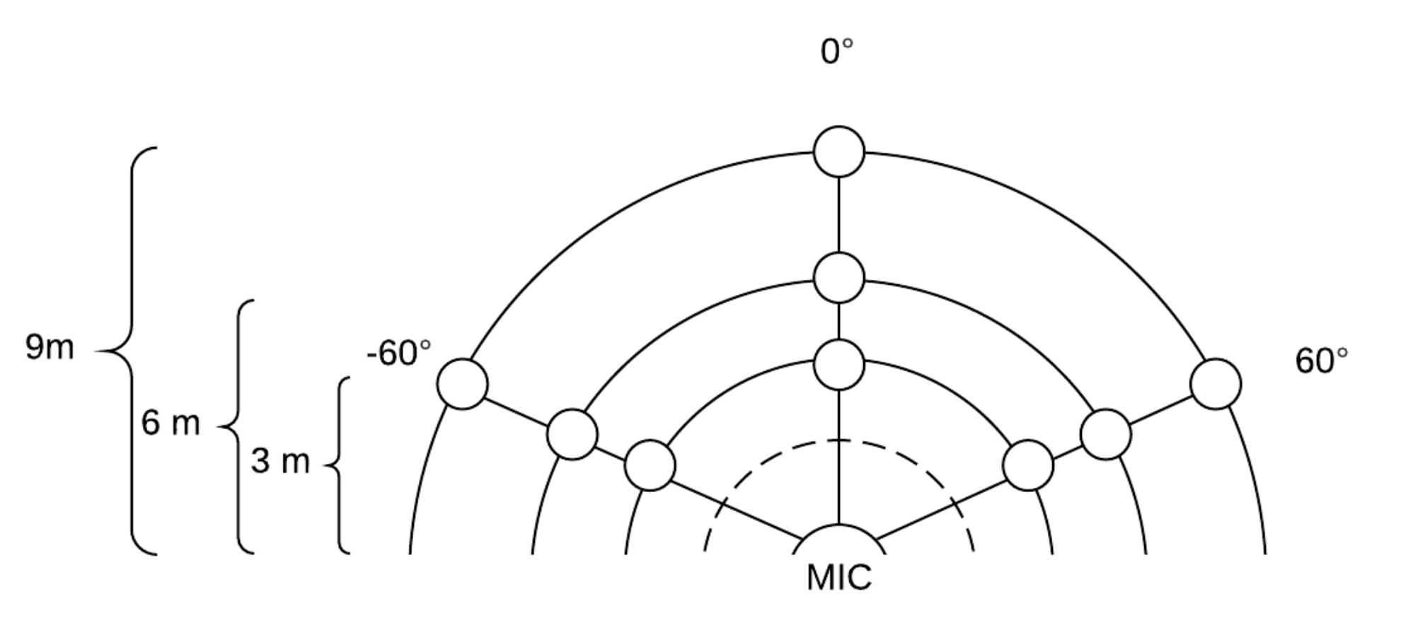
• Set up the base to its maximum height and point it to an angle of 45${}^{\circ }$ with respect to the base.
• Set the data acquisition points with masking tape in the ground, starting from −60${}^{\circ }$ and marking a point for 3 m, 6 m and 9 m with respect to the base location, and repeat the process for angles 0${}^{\circ }$ and 60${}^{\circ }$ for a total of 9 points as is shown in Figure 2.
• Start to record the audios with the data acquisition program.
• Position the subject in the initial starting point, that is, (−60${}^{\circ }$, 3 m), and ask them to scream the predefined expressions SN, HN and AN.
• Repeat the process for the following points.
• Stop recording the data.

The experiment was conducted on university undergraduate students ranging in age from 18 to 25 years in Colombia, South America. It was approved by the “Universidad de los Andes” ethics committee “Comité de Ética de la Investigación”. The experiment included audio recordings from 18 male and 5 female subjects. We chose students in this experiment due to the fact that they are the main population that transits the area where the experiment was being held. Every audio recording for a single subject included 27 positive distress signals and several background signals. The final dataset contains 24 audio files from 23 different subjects of about 2 min each, recorded at 22,050 Hz, with a total duration of around 48 min. A total of 648 positive events per class were collected.

Table 1. Class distribution of the samples in the database.

Class	Number of Samples	Percentage
BN	20,645	82.04%
SN	1228	4.88%
AN	1771	7.04%
HN	1521	6.04%

shows the class distribution in the dataset.

As it is intended to create an affordable device, the chosen hardware needs to be low cost. Therefore, the selected elements were as follows.

• Snowball iCE Condenser microphone, Pressure Gradient With USB digital output. This has a cardioid profile with an even frequency response for human voice range to reduce the misdetection of distress signals.
• 3.5 m long Type-A to Type-B USB cable.
• 3 m long microphone base.

2.3. Feature Extraction

It has been found that both time and frequency analysis provide informative features for speech recognition [16]. Two of the widely used time and frequency ways audio signals are processed are the Mel spectrogram [17] and Mel frequency cepstral coefficients [18]. These features that are extracted from the audio signals will eventually feed the convolutional neural networks to conduct the classification task. In the following, we provide a brief explanation of how these features are computed.

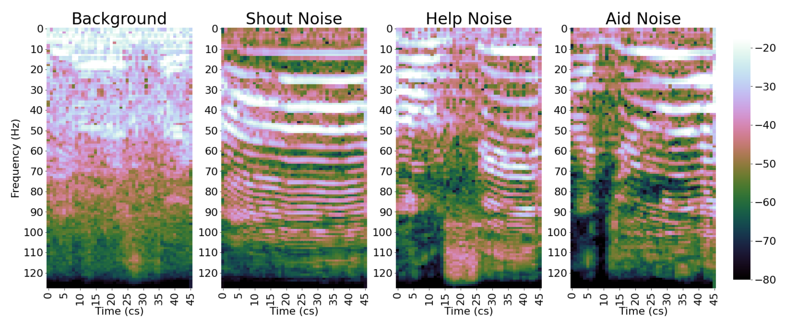
2.3.1. Mel Spectrogram

This is a 2-dimensional signal where its variables are time and frequency. To compute this spectrogram, first, the short-term Fourier transform is computed over a series of overlapping windows of the audio signal, obtaining a representation that shows the frequency content of the signal as it changes over time. Then, frequencies are scaled according to the Mel’s scale [19]. This scale tries to resemble human’s perception of pitches and can be computed using the following equation.

$$F_{mel}=\frac{1000}{log\left(2\right)}log\left(1+\frac{F_{hz}}{1000}\right)$$

(1)

The Mel spectrogram was obtained from the input audio data that we collected in our database for each class: background and three types of calls for help. Figure 3 illustrates the computation of the Mel spectrogram from a sample of each category. Note that this 2-dimensional representation of the audio signals evidences distinguishing patterns for each one of the proposed classes.

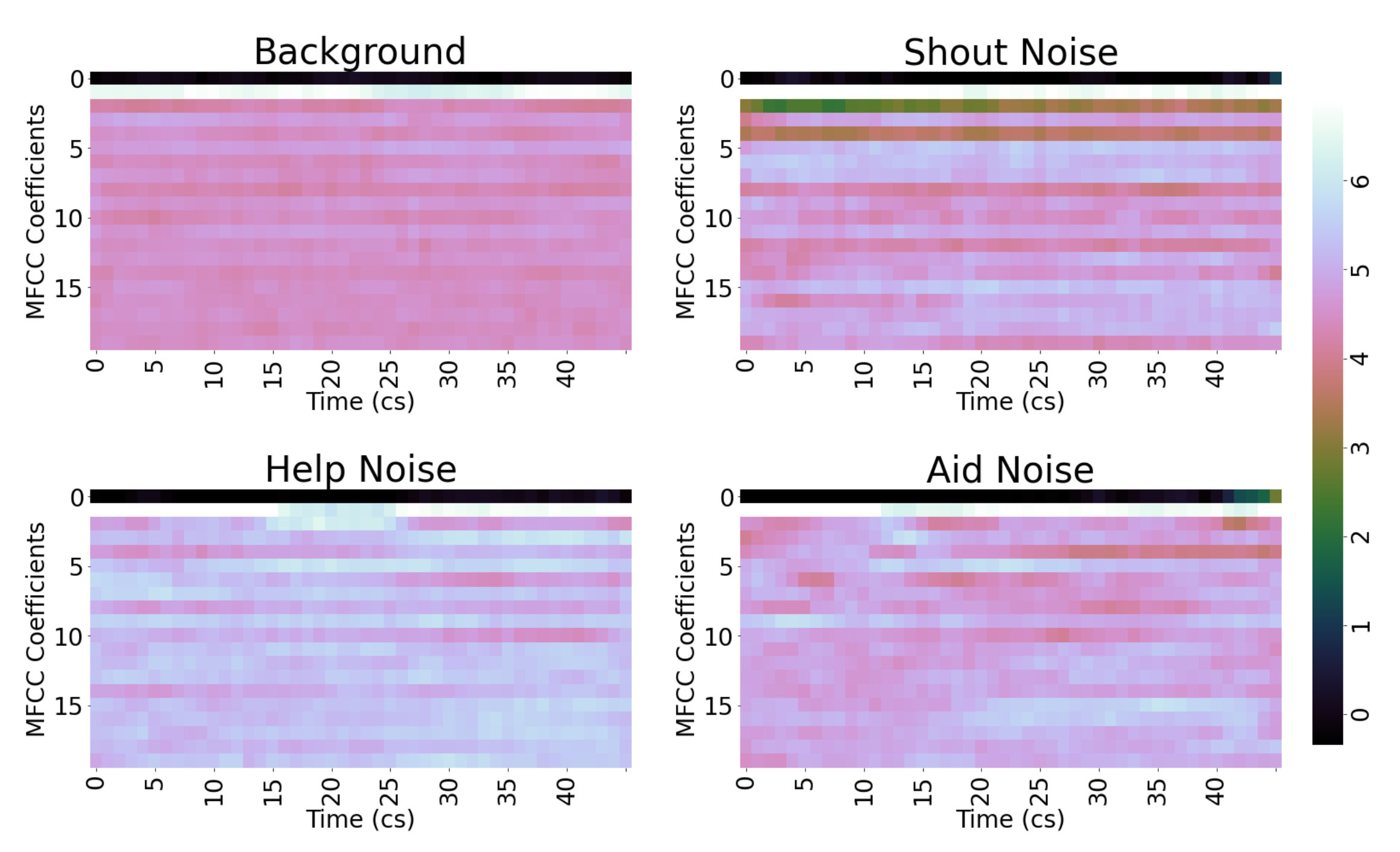
2.3.2. Mel Frequency Cepstral Coefficients

Mel Frequency Cepstral Coefficients (MFCCs) correspond to the discrete cosine transform of a Mel frequency spectrogram. They provide an alternative representation of the Mel frequency spectrogram. Figure 4 shows the coefficients for samples that belong to each class. As in the case of the Mel spectrogram, MFCCs evidence distinguishing patterns for each one of the proposed classes.

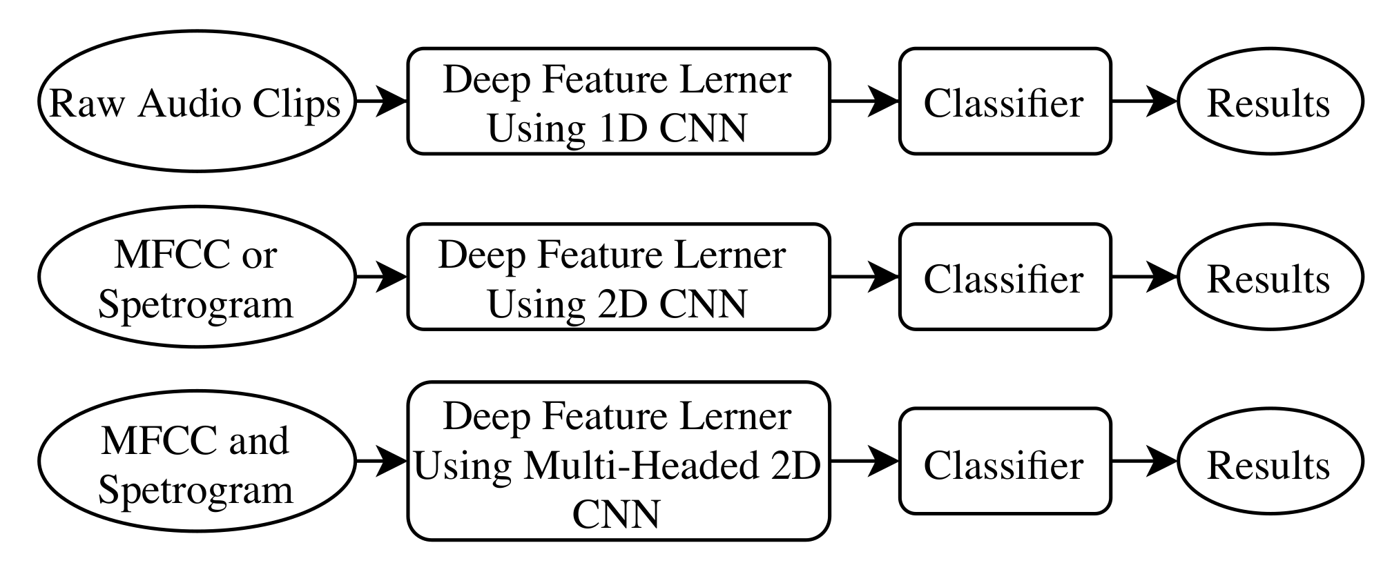
2.4. Convolutional Neural Network (CNN) Architectures

Now, we present the network architectures that were implemented to solve the classification problem. We evaluated a 1-dimensional Convolutional Neural Network (CNN) and three types of 2-dimensional CNNs. A CNN is a neural network that uses filtering operations to extract information from raw signals to facilitate finding those patterns that allow an accurate classification task [20]. The main difference between the 1D and 2D CNN is the structure of the input information, and how the filters are applied on the input signal. While the 1D CNN filter only operates on a one-dimensional signal, the 2D CNN filter operates on a bidimensional signal. Figure 5 shows block diagrams summarizing the network architectures that were evaluated.

2.4.1. 1D CNN

The input of this network corresponds to a given window of the raw audio signal. The network is composed of 3 layers in which a convolution with a ReLU activation function is followed by a max pool stage. A flatten layer is added, followed by a dropout layer for regularization. Then, four consecutive dense layers are implemented, where the first three have 20 neurons each and a ReLU activation function, and the last one has 4 neurons (one per class) and a softmax activation function.

2.4.2. 2D CNN

We implemented two networks, one whose input is the Mel spectrogram, and another whose input are the MFCCs. The configuration of the proposed CNNs is similar to the one used in the 1D CNN, containing 3 layers that compute convolutions and max pooling.

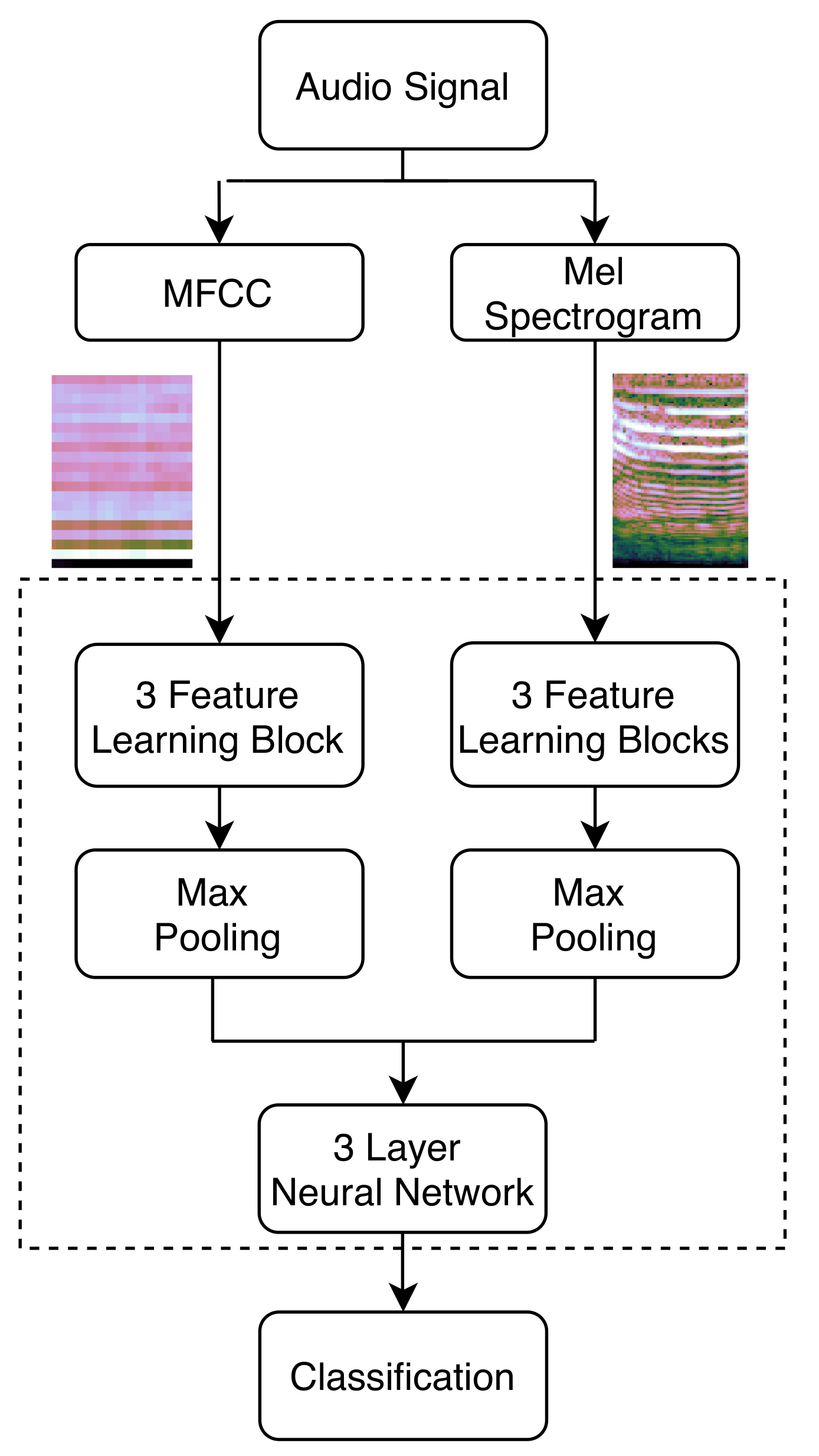
2.4.3. Multi-Headed CNN

The data collected from the Mel spectrogram and the Mel frequency ceptral coefficients are combined as a single input to learn global features of the sounds in this architecture. Each head of the multi-headed 2D network has several feature learning blocks that consist of one convolutional layer and one batch normalization layer to improve training speed and the stability of the network. This architecture is composed of 3 feature learning blocks at each branch, followed by a max pooling layer that allows the network to be robust against noise and distortions. After this, a DropOut layer is used in order to regularize the network and prevent it from overfitting. The data of the two networks are then flattened and concatenated, providing the input of a three phase neural network. At last, a neural layer with activation softmax is connected to make the final predictions. A simplified diagram of this architecture can be seen in Figure 6.

3. Results

The networks were trained off-line using google-colab resources, where the final design was obtained by tuning the parameters using a grid search. At the end of each of the architectures, a softmax function is used to make the classification between the four possible sounds. When the networks are trained and the process of validation is completed, we made tests on the RaspberryPi.

Before showing the experimental results on the proposed methods on the collected database, we compared the performance of the proposed system to the one achieved by the method presented in [8] to justify the use of CNN as classification model. The work in [8] is the closest research work to ours that we found in the literature, and it employs an SVM classifier with soft assignment on both the Mel spectrogram and MFCCs. To compare these methods, we applied our multi-headed 2D CNN to the database collected by them. This database was sampled at 32 KHz and has a sample resolution of 16 bits. Audios were recorded using a high-quality microphone. It contains three classes of audio events that have to be detected: screams, glass breaking, and gun shot. Background noise was artificially added to the audio files. A summary of the composition of their database is reported in

Table 2. Summary of the composition of the dataset created in [8].

	Training Set		Test Set
	# Events	Duration (s)	# Events	Duration (s)
BN	-	58,371.6	-	25,036.8
GB	4200	6024.8	1800	2561.7
GB	4200	1883.6	1800	743.5
S	4200	5488.8	1800	2445.4

, where the abbreviations GB, GS, S and BN correspond to Glass Breaking, gunshot, scream, background noise respectively.

We also used the same evaluation criterion as in [8], in which an event is considered as correctly detected if it is detected in at least one of the sliding time windows that overlap with it. If in two consecutive time windows a foreground event is detected, a single false positive occurrence is counted [8]. We resampled audio data to 22,050 Hz.

Table 3. Results reported in [8] in their database.

		Predicted Class
		GB	GS	S	BN
True Class	GB	94.4%	0.2%	0.2%	5.2%
	GS	3.5%	84.9%	0.5%	11.1%
	S	2.6%	0.9%	80.8%	15.7%
	BN	-	-	-	97.4%

and

Table 4. Results achieved by our multi-headed 2D CNN applied to the data-base collected in [8].

		Predicted Class
		GB	GS	S	BN
True Class	GB	92.8%	0.0%	0.0%	7.2%
	GS	0.33%	85.67%	0.0%	14.0%
	S	0.0%	0.0%	86.0%	14.0%
	BN	0.33%	0.1%	0.48%	99.09%

show the results on their database using SVM, as it was proposed in Table 3, and our CNN, respectively. Table 3 does not show results refereed to false positives for BN because the results were not reported in [8]. The average recognition rate of events achieved in [8] is 86.7% with a 2.6% of false positive rate, which is lower than the one achieved using our method which is 88.16% with a 0.91% of false positive rate. The CNN clearly outperforms a SVM in this classification task.

Now that we justified the use of CNN as classification model, we evaluated the performance of the proposed architectures on our database. The validation process is based on a k-fold cross-validation scheme. Each fold contains the audio files from one person to guarantee independent samples in the training set. Then, we have 8 folds, each one containing 27 events for each class. The classification task is conducted on 450 ms time windows, with 112 ms of overlap. This window frame was selected considering that, to recognize distress signals, the window should be long enough to collect information that allows for discrimination. Taking this into account, every type of sound takes the same amount of time to process because all time windows are the same. To evaluate the classification models, we considered the recognition rate of each frame window and the false positive rate.

3.1. Performance 1D CNN

We proposed a 1D CNN as a first approach due to the simplicity of the data extraction. Using this architecture and using the raw data from our database, we registered the confusion matrix shown in

Table 5. Results achieved 1D CNN.

		Predicted Class
		BN	SN	HN	AN
True Class	BN	94%	1.4%	1.6%	2.6%
	SN	9.8%	63%	5.5%	21%
	HN	12%	5.9%	63%	19%
	AN	13%	16%	18%	53%

. From these results, it is clear that extra processing on the audio data is needed to achieve better results using CNN. The average recognition rate of the events of interest was only 59.67%, while the false positive rate has a value of 5.6%. For this reason, and the fact that commonly used speech recognition features are extracted from MFCCs and the Mel spectrogram, a 2D CNN was our next proposed approach.

3.2. Performance 2D CNN

We tested the performance of the 2D CNN in our dataset. The confusion matrix for the 2D architecture applied to the MFCCs is shown in

Table 6. Results achieved by the 2D CNN and MFCCs as input.

		Predicted Class
		BN	SN	HN	AN
True Class	BN	94%	1.5%	2.5%	1.6%
	SN	8.8%	66%	12%	12%
	HN	7.3%	3.5%	81%	8.1%
	AN	10%	14%	15%	61%

, and the confusion matrix achieved using the Mel spectrogram is shown in

Table 7. Results achieved by the 2D CNN and Mel spectrogram as input.

		Predicted Class
		BN	SN	HN	AN
True Class	BN	96%	0.92%	1.2%	1.4%
	SN	10%	73%	4.5%	12%
	HN	8.6%	4%	76%	11%
	AN	7.6%	10%	5.6%	77%

. The average recognition rates of events using this architecture were 69.3% and 75.3% with false positive rates of 5.6% and 3.52% for the 2D CNN using MFCCs and Mel spectrogram as inputs, respectively. These results show that this architecture presents a clear improvement over the 1D CNN, especially when the Mel spectrogram is used as an input.

3.3. Performance Multi-Headed 2D CNN

The confusion matrix in

Table 8. Results achieved Multi-headed 2D CNN.

		Predicted Class
		BN	SN	HN	AN
True Class	BN	96%	1.3%	1.4%	1.1%
	SN	7.7%	79%	3.1%	10%
	HN	5%	3.1%	84%	6.7%
	AN	5.5%	9.7%	8.3%	76%

shows the performance of considering both the Mel spectogram and MFCCs in one process. Performance is better than both 2D CNN models. The average recognition rate of the model is 79.67%, which means an improvement of 4.37% in average. The detection of events of interest using this method is 94% if we group the three classes of shouting events together.

3.4. Prototype Implementation

We assessed the performance of the real-time recognition system composed of the low-cost microphone and a Raspberry Pi with the trained model. The network model that was trained off-line was deployed on the Raspberry Pi using Tensorflow Lite, which has been shown to have a good performance behavior on this type of devices [21]. This device takes a batch of audio samples every 450 milliseconds, which is passed through a preprocessing stage that computes the Mel spectrogram and MFCCs. The result of this computation corresponds to the input of the multi-headed CNN, which provides a prediction of the class in a given window. We computed some performance indicators to measure the feasibility of computation of our classification model on the Raspberry Pi: audio recollection time, which is the time to acquire the audio samples for a given window; data preprocessing time, which is the time needed to extract the MFCC and Mel spectrogram given the audio signal; prediction time, which is the time needed to compute the network operations to provide a prediction; and RAM consumption of the model.

Table 9. Mean computational costs of the proposed device implementation.

Audio recollection time	450 ms
Pre-processing time	43 ms
Prediction time	63 ms
Memory	635 MB

summarizes the mean average computational costs of the proposed device implementation for 100 audio windows.

These results show that the portable implementation of the model in the Raspberry Pi is adequate to give a quick response in the task of event recognition, which can be considered as real-time processing. These results are comparable to the ones obtained by other works that implemented real-time applications of audio processing. Examples include audio processing times for real-time predictions of around 1000 ms in [6], and between 104 to 1360 ms in [22].

4. Conclusions

We designed a portable device for audio distress signal identification in urban areas. The process resulted in a database in Spanish language with the shouts recorded in a real setting with low-cost resources, a deep learning model that the validation proved successful in a real situation, and a proposed implementation of the low-cost device using a Raspberry Pi. The performance of the multi-headed CNN proved to be more accurate that other methods in detecting shouted speech and than only using raw audio features. The model was tested on two different datasets and gave positive results on both, as it can successfully distinguish between background noise and relevant data. Furthermore, a Raspberry Pi was shown to be adequate in terms of processing time to implement a device for real-time processing. Putting all the pieces together, we designed a low-cost and portable device capable of detecting audio distress signals in noisy environments. The implementation and widespread of such a device can positively affect smart cities by reducing response times in distress situations.

Future work includes the implementation of networks with different architectures, such as a multi-headed CNN that uses the combined information of MFCCs, Mel spectrogram, and raw audio data; recurrent neural networks; and long short-term memory networks. It is important to study techniques to reduce the complexity of the network such as pruning to reduce the processing times. To provide better classification results, it is useful to expand the database using low-cost devices and real-world scenarios. Future studies should incorporate and evaluate IoT technologies into the system and recent acoustic sensors for outdoor noise monitoring [23] that have been developed. Moreover, the effect of changing sociodemographic variables can be explored, adding more age groups, education levels, and diverse cultural background in the database.

References

1. Vidal, J.B.I.; Kirchmaier, T. The Effect of Police Response Time on Crime Detection; Cep Discussion Papers; Centre for Economic Performance, LSE: London, UK, 2015. [Google Scholar]
2. Mabrouk, A.B.; Zagrouba, E. Abnormal behavior recognition for intelligent video surveillance systems: A review. Expert Syst. Appl. 2018, 91, 480–491. [Google Scholar] [CrossRef]
3. Eng, H.L.; Toh, K.A.; Yau, W.Y.; Wang, J. DEWS: A live visual surveillance system for early drowning detection at pool. IEEE Trans. Circuits Syst. Video Technol. 2008, 18, 196–210. [Google Scholar]
4. Mubashir, M.; Shao, L.; Seed, L. A survey on fall detection: Principles and approaches. Neurocomputing 2013, 100, 144–152. [Google Scholar] [CrossRef]
5. Burkhardt, F.; Paeschke, A.; Rolfes, M.; Sendlmeier, W.F.; Weiss, B. A database of German emotional speech. In Proceedings of the Ninth European Conference on Speech Communication and Technology, Lisbon, Portugal, 4–8 September 2005; pp. 1517–1520. [Google Scholar]
6. Huang, W.; Chiew, T.K.; Li, H.; Kok, T.S.; Biswas, J. Scream detection for home applications. In Proceedings of the 2010 5th IEEE Conference on Industrial Electronics and Applications, Taichung, Taiwan, 15–17 June 2010; pp. 2115–2120. [Google Scholar]
7. Parsons, C.E.; Young, K.S.; Craske, M.G.; Stein, A.L.; Kringelbach, M.L. Introducing the Oxford Vocal (OxVoc) Sounds database: A validated set of non-acted affective sounds from human infants, adults, and domestic animals. Front. Psychol. 2014, 5, 562. [Google Scholar] [CrossRef] [PubMed] [Green Version]
8. Foggia, P.; Petkov, N.; Saggese, A.; Strisciuglio, N.; Vento, M. Reliable detection of audio events in highly noisy environments. Pattern Recognit. Lett. 2015, 65, 22–28. [Google Scholar] [CrossRef]
9. Poria, S.; Cambria, E.; Howard, N.; Huang, G.B.; Hussain, A. Fusing audio, visual and textual clues for sentiment analysis from multimodal content. Neurocomputing 2016, 174, 50–59. [Google Scholar] [CrossRef]
10. Strisciuglio, N.; Vento, M.; Petkov, N. Learning representations of sound using trainable COPE feature extractors. Pattern Recognit. 2019, 92, 25–36. [Google Scholar] [CrossRef] [Green Version]
11. Dhanalakshmi, P.; Palanivel, S.; Ramalingam, V. Pattern classification models for classifying and indexing audio signals. Eng. Appl. Artif. Intell. 2011, 24, 350–357. [Google Scholar] [CrossRef]
12. Zhao, J.; Mao, X.; Chen, L. Speech emotion recognition using deep 1D & 2D CNN LSTM networks. Biomed. Signal Process. Control 2019, 47, 424. [Google Scholar]
13. Alarcón-Paredes, A.; Francisco-García, V.; Guzmán-Guzmán, I.P.; Cantillo-Negrete, J.; Cuevas-Valencia, R.E.; Alonso-Silverio, G.A. An IoT-Based Non-Invasive Glucose Level Monitoring System Using Raspberry Pi. Appl. Sci. 2019, 9, 3046. [Google Scholar] [CrossRef] [Green Version]
14. Ou, S.; Park, H.; Lee, J. Implementation of an obstacle recognition system for the blind. Appl. Sci. 2020, 10, 282. [Google Scholar] [CrossRef] [Green Version]
15. Blue Microphones Snowball USB Microphone User Guide. 2009. Available online: https://s3.amazonaws.com/cd.bluemic.com/pdf/snowball/manual.pdf (accessed on 1 June 2020).
16. Chou, W.; Juang, B.H. Pattern Recognition in Speech and Language Processing; CRC Press: Boca Raton, FL, USA, 2003. [Google Scholar]
17. Piczak, K.J. The details that matter: Frequency resolution of spectrograms in acoustic scene classification. In Detection and Classification of Acoustic Scenes and Events; Warsaw University of Technology: Munich, Germany, 2017; pp. 103–107. [Google Scholar]
18. Kadiri, S.R.; Alku, P. Mel-Frequency Cepstral Coefficients of Voice Source Waveforms for Classification of Phonation Types in Speech. In Interspeech; Department of Signal Processing and Acoustics, Aalto University: Espoo, Finland, 2019; pp. 2508–2512. [Google Scholar]
19. Umesh, S.; Cohen, L.; Nelson, D. Frequency warping and the Mel scale. IEEE Signal Process. Lett. 2002, 9, 104–107. [Google Scholar] [CrossRef]
20. Lecun, Y.; Bengio, Y.; Hinton, G. Deep Learning; MIT Press: Cambridge, UK, 2015. [Google Scholar] [CrossRef]
21. Velasco-Montero, D.; Fernández-Berni, J.; Carmona-Galán, R.; Rodríguez-Vázquez, Á. Performance analysis of real-time DNN inference on Raspberry Pi. In Proceedings of the Real-Time Image and Video Processing 2018. International Society for Optics and Photonics, Taichung, Taiwan, 9–12 December 2018; Volume 10670, p. 106700F. [Google Scholar]
22. Arslan, Y. A New Approach to Real Time Impulsive Sound Detection for Surveillance Applications. arXiv 2019, arXiv:1906.06586. [Google Scholar]
23. López, J.M.; Alonso, J.; Asensio, C.; Pavón, I.; Gascó, L.; de Arcas, G. A Digital Signal Processor Based Acoustic Sensor for Outdoor Noise Monitoring in Smart Cities. Sensors 2020, 20, 605. [Google Scholar] [CrossRef] [PubMed] [Green Version]
Figure 1. Diagram of the proposed device: Two meter tall structure containing the Raspberry Pi and the microphone slightly tilted forward.
Applsci 10 07448 g001
Figure 2. Diagram for data collection points spatial distribution.
Applsci 10 07448 g002
Figure 3. Mel spectrogram in a window of 45 cs for each category. Horizontal axis corresponds to time and vertical axis corresponds to frequency. Darker colors indicate lower magnitude values.
Applsci 10 07448 g003
Figure 4. Mel Frequency Cepstral Coefficients in a window of 45 cs for each category. Horizontal axis corresponds to time and vertical axis corresponds to the magnitude of the coefficients. Darker colors indicate lower magnitude values.
Applsci 10 07448 g004
Figure 5. Flow charts of the distress signal recognition approaches adopted in this paper from top to bottom: Classifier using 1D CNN with features extracted from raw data; Classifier using 2D CNN with features extracted from Spectrogram or MFCCs; Classifier using Double 2D CNN with features extracted from Mel spectrogram and MFCCs.
Applsci 10 07448 g005
Figure 6. Block Diagram of the designed Multi-Headed 2D Convolutional Neural Network (CNN).
Applsci 10 07448 g006