Research on Passive Ranging Technology of Moving Ship Based on Vertical Hydrophone Array

Abstract

This paper introduces a method for the range localization of a moving ship based on the vertical hydrophone line array. The main implementation steps of the proposed algorithm are as follows. First, the stable low-frequency line spectrum component of the broadband radiated noise from the moving ship was extracted through the Detection of Envelope Modulation on Noise (DEMON) spectrum analysis method. Second, the pressure difference between the two different ranges was derived, and the corresponding interference fringes were observed in the plane of time and time interval. Then, the radial velocity of the moving ship could be obtained based on the period of the pattern oscillations of the interference fringes. Further, we estimated the time and range information of the Closest Point of Approach (CPA) and computed the ship range versus time. Finally, each element of the vertical hydrophone line array was processed by the method proposed above, and data fusion technology was adopted to reduce the impact of ineffective elements and improve the range estimation accuracy. The results of the simulation and experiment of a 16-element vertical array performed in the South China Sea verified the effectiveness of the algorithm.

1. Introduction

Range localization is a significant component of the Sound Navigation and Ranging (SONAR) system in the field of underwater target detection. Currently, the most popular methods for ranging are three subarrays, the matched field processing (MFP) and the waveguide invariant method. The three subarray passive ranging method mainly uses the principle of the curvature of the spherical wavefront. The target range is estimated by measuring the relative time delay of the received signal on each of the three subarrays [1]. However, this method is easily affected by the time delay estimation accuracy, whose error cannot be ignored, especially in the complex ocean environment [2]. The matching field passive positioning technology is an environment-dependent method based on ocean channel modelling [3]. The copy sound field is first calculated through the ocean channel model, and the matching processing is applied in the copy field and signals received by the hydrophone array. We can obtain the range and depth information of the sound source after the parameter search processing [4,5]. However, the mismatch problem of the ocean channel environment cannot be solved effectively in practice, and thus the matching field positioning accuracy becomes poor. Comparatively, the waveguide invariant technology is more tolerant of the environmental demands, which is an important parameter to describe the range-frequency interference structure phenomenon of the ocean sound field. Cockrell [6] adopted the waveguide invariant technology to estimate the range of a broadband sound source by using a single hydrophone. This method requires only a little prior knowledge of the environment and acquires a higher estimation accuracy. Reference [7] developed a method to achieve range localization in shallow water and a range-independent environment when the time interval of the pressure field was ascertained. Rémi et al. [8] adopted the waveguide invariant theory to achieve the orientation by quantifying the intensity interference fringes in the range-frequency domain. Furthermore, the waveguide invariant parameter is the core of the spectral analysis that is involved in the range estimation. The signal transmitted from cargo ships can be used to estimate both the time-varying source-receiver range and the receiver position [9].

Further, many robust algorithms have been developed to improve range estimation precision. Li [10] employed the Low Frequency Analysis Record (LOFAR) spectrum of the vector sensor linear array to record the parabolic striations of the wide-band target passing the CPA point. Then, the image processing technology was used to obtain the waveguide invariance and realize the range estimation of the target. Cho et al. [11] combined the waveguide invariant with the beam-time migration technology to achieve a range estimation by a vertical or horizontal array.

Generally, the sound sources mentioned in the above literature mostly radiate narrowband or broadband signals. In comparison with the wideband ship noise, the narrowband ship noise is more extensively applied in the range estimation field. However, the low-frequency line spectrum of the broadband ship noise is usually unstable, and it needs to be preprocessed by signal processing technology in order to obtain a high SNR narrowband signal. The Detection of Envelope Modulation on Noise (DEMON) spectrum method is widely used in the analysis of broadband ship noise, and the low-frequency characteristic spectrum can be obtained by demodulating the high-frequency components of the receiving signal [12,13,14].

Due to the poor ranging accuracy of a single hydrophone, researchers developed multi-sensor data fusion technology. Data fusion is defined as a technology that combines data from multiple sensors with information from related databases to achieve a higher precision [15]. In the middle of the 20th century, this technology was introduced into the underwater acoustic field and was mainly used for underwater detection, target recognition and underwater localization. Li et al. [16] fused the data from bow and side arrays to improve the detection performance with a low signal-to-noise ratio (SNR). Dos Santos et al. [17] applied the fusing data from several image domains to realize underwater localization. They also combined deep neural networks with adaptive Monte Carlo localization technology. Reference [18] discussed the target localization problem in underwater sensor networks and designed a deterministic weight for consensus fusion in order to mitigate the malicious measurements. The experiment results after four sensor fusions validated that the fusion of measurements was significant due to smaller localization errors. Prasanna et al. [19] adopted the Modified Gain Bearings only Extended Kalman filter (MGBEKF) algorithm to judge whether there were one or two targets. This method made use of various sensors such as the structure-mounted array and towed array to perform the state vector fusion.

In this paper, we propose a range localization method of a moving target based on a vertical hydrophone line array. A simulation and sea experiment of a 16-element vertical hydrophone array in the deep sea were conducted. Both results indicate that this algorithm can estimate the range and achieve more accurate results.

This paper is organized as follows. In Section 2, we introduce the basic theory of this ranging technology. A simulation is performed to evaluate the performance of the proposed algorithm. Section 4 discusses the sea trial results. Section 5 gives a summary.

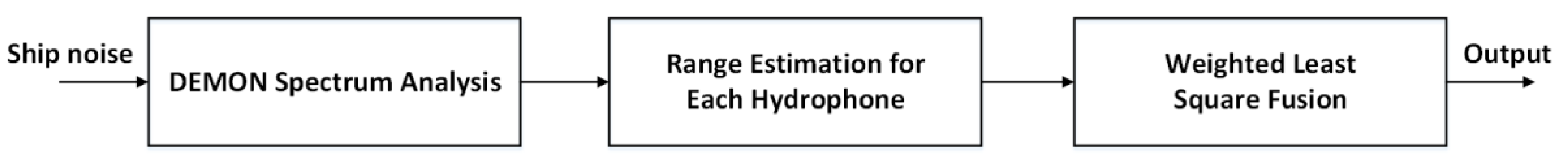
2. Basic Theory

The range localization method includes three steps. First, DEMON spectrum analysis is employed to extract the low-frequency line spectrum components from the wideband ship noise. Second, the range localization can be achieved based on the intensity of the sound pressure difference over the time interval. Finally, the weighted least square (WLS) fusion method is applied to fuse the multi-hydrophone ranging results. The flow diagram is as shown in Figure 1.

2.1. DEMON Spectrum Analysis for A Single Hydrophone

As mentioned above, the DEMON spectral analysis is widely used in the feature extraction of ship-radiated noise. Generally speaking, the high-frequency band of the vessel-radiated noise has a periodic modulation, and the modulation frequency is composed of low-frequency characteristic signals such as the shaft frequency and blade frequency. The shaft frequency and blade frequency contain the information on the propeller speed and blade number. Normally, the ship-radiated noise is a periodic and locally stable process, whose expression in the time domain can be expressed as:

$$x\left(t\right)=\left[1+f\left(t\right)\right]\cdot g\left(t\right)$$

(1)

where $f\left(t\right)$ represents the modulation signal and is a low-frequency, slowly varying periodic function. $g\left(t\right)$ is the carrier frequency and is a stable White Gaussian random process with a limited bandwidth. $x\left(t\right)$ is a periodic stationary stochastic Gaussian process for ship-radiated noise. The modulation signal $f\left(t\right)$ can be obtained by demodulating the ship noise $x\left(t\right)$. This paper adopts the absolute value demodulation technology of the incoherent demodulation method. The specific flow diagram has been presented in Figure 2.

The process includes four steps: band-pass filtering, the operation of taking the absolute value, the low-pass filter, the spectrum analysis.

We take a simple situation as an example to explain the operation principle. In this case, the amplitude of the high-frequency carrier is modulated, and the carrier signal is a single frequency signal. The amplitude modulation (AM) signal is expressed as:

$$x\left(t\right)=A_m\cos \left(2\pi f_{m}t\right)\left[1+A_c\cos \left(2\pi f_{c}t\right)\right]$$

(2)

where $A_m$ and $A_c$ are the amplitude of the carrier signal and modulation signal, respectively. Moreover, we assume that $A_m$ and $A_c$ are both greater than one. $f_m$ and $f_c$ are the frequency of the carrier signal and modulation signal, respectively.

Taking the absolute value of Equation (2), the AM signal can be written as:

$$\left|x\left(t\right)\right|=A_m\left|\cos \left(2\pi f_{m}t\right)\right|\left|1+A_c\cos \left(2\pi f_{c}t\right)\right|$$

(3)

Then, the content of the absolute value is expanded into a Fourier series, that is:

$$\left|\cos \left(2\pi f_{m}t\right)\right|=A_0+A_1\sin \left(2\pi f_{m}t\right)+A_2\sin \left(2\pi \cdot 2f_{m}t\right)+\cdots$$

(4)

$$\left|1+A_c\cos \left(2\pi f_{c}t\right)\right|=B_0+B_1\sin \left(2\pi f_{c}t\right)+B_2\sin \left(2\pi \cdot 2f_{c}t\right)+\cdots$$

(5)

where $A_n$ and $B_n$ are the constant coefficients. The multiplication of Equations (4) and (5) will produce various harmonic components. After passing through the designed low-pass filter, only the modulated signal remains. Then, the spectrum analysis of the low-frequency modulation signal is carried out after a Fourier transform.

According to the spectrum distribution, we extract the line spectrum components representing the characteristics of the ship for the next step of the ranging analysis.

2.2. Range Estimation by Sound Intensity of The Pressure Difference

In the acoustic field, the intensity of the pressure difference received at different ranges contains information about the range interval, from which the radial velocity of the moving target can be obtained. Then, the range over time can be estimated.

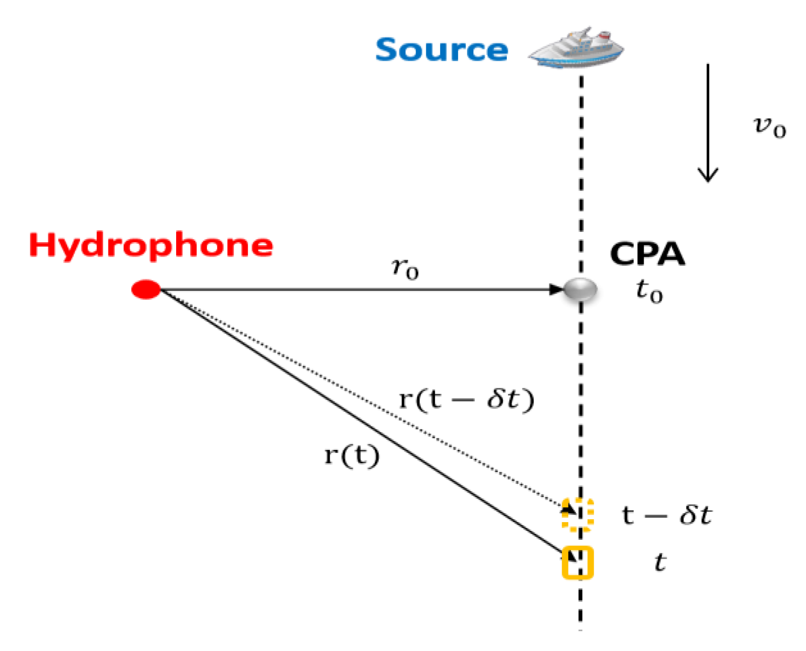
2.2.1. Radial Velocity Derivation

According to the normal wave model theory, the sound pressure at a certain receiving depth $z$ and range $r$ in the sound field can be expressed as [20]:

$$p\left(r,z\right)=\frac{i}{\rho \left(z_s\right)\sqrt{8\pi r}}{e}^{-i\pi /4}{\displaystyle \sum _{m=1}^{\infty }{\mathsf{\Psi }}_m\left(z_s\right)}{\mathsf{\Psi }}_m\left(z\right)\frac{e^{i{k}_{rm}r}}{\sqrt{k_{rm}}}$$

(6)

where $z_s$ is the source depth, $\rho$ is the density of sea water and $m$ stands for the pattern number. ${\mathsf{\Psi }}_m\left(z\right)$ and ${\mathsf{\Psi }}_m\left(z_s\right)$ are the eigenfunction of the $m$-th pattern for the source depth and receiving depth, respectively. $k_{rm}$ represents the eigenvalue.

Similarly, the sound pressure at a close range $r+\Delta r$ can be expressed as:

$$p\left(r+\Delta r,z\right)=\frac{i}{\rho \left(z_s\right)\sqrt{8\pi \left(r+\Delta r\right)}}{e}^{-i\pi /4}{\displaystyle \sum _{m=1}^{\infty }{\mathsf{\Psi }}_m\left(z_s\right)}{\mathsf{\Psi }}_m\left(z\right)\frac{e^{i{k}_{rm}\left(r+\Delta r\right)}}{\sqrt{k_{rm}}}$$

(7)

where $\Delta r$ is a small amount. We define the middle range as $R=r+\Delta r/2$ and assume $\Delta r/2\ll R$.

Therefore, the pressure difference between the range $r$ and $r+\Delta r$ in the same receiving depth is [7]:

$$\begin{array}{ccc}\Delta p\left(R,\Delta r\right)& =& p\left(r+\Delta r\right)-p\left(r\right)\hfill \\ & =& A\cdot {\displaystyle \sum _{m=1}^{\infty }{B}_m}{e}^{i{k}_{rm}R}\sin \left(k_{rm}\frac{\Delta r}{2}\right)\end{array}$$

(8)

where $A=\frac{-e^{-i\pi /4}}{\rho \left(z_s\right)\sqrt{2\pi }}$ is a constant, and $B_m=\frac{{\mathsf{\Psi }}_m\left(z_s\right){\mathsf{\Psi }}_m\left(z\right)}{\sqrt{k_{rm}R}}$ is unrelated to the range interval $\Delta r$. The sound intensity of the pressure difference can be indicated as:

$$\begin{array}{ccc}{I}_{\Delta }\left(R,\Delta r\right)& =& \left(\Delta p\left(R,\Delta r\right)\right)\cdot {\left(\Delta p\left(R,\Delta r\right)\right)}^{\ast }={\left|\Delta p\left(R,\Delta r\right)\right|}^2\hfill \\ & =& {\left|A\right|}^2{\displaystyle \sum _m{\displaystyle \sum _n{A}_m}{A}_n}\left[\cos \left(\left(k_{rm}-k_{rn}\right)\frac{\Delta r}{2}\right)-\cos \left(\left(k_{rm}+k_{rn}\right)\frac{\Delta r}{2}\right)\right]\cdot \cos \left[\left(k_{rm}-k_{rn}\right)R\right]\end{array}$$

(9)

It is noted that the period of the $\cos \left(\left(k_{rm}-k_{rn}\right)\frac{\Delta r}{2}\right)$ is much longer than that of the term $\cos \left(\left(k_{rm}+k_{rn}\right)\frac{\Delta r}{2}\right)$. Thus, the sound intensity of the pressure difference is mainly dominated by the latter term. The simplified expression is as follows:

$$I_{\Delta }\left(R,\Delta r\right)={\left|A\right|}^2{\displaystyle \sum _m{\displaystyle \sum _n{A}_m}{A}_n}\left[\cos \left(\left(k_{rm}+k_{rn}\right)\frac{\Delta r}{2}\right)\right]\cdot \cos \left[\left(k_{rm}-k_{rm}\right)R\right]$$

(10)

Further, we define $k_{ri}=\delta k_i+ {\overline{k}}_r,i=m,n$, where $\delta k_i$ is a minimal quantity and ${\overline{k}}_r$ is the average wave number of the modes. Its value is between $k_{\min }=\frac{\omega }{c_b}$ and $k_{\max }=\frac{\omega }{\min \left(c_w\right)}$, where $c_b$ and $c_w$ are the sound speed at the bottom surface and in the water layer, respectively.

Thus, Equation (10) can be further expressed as:

$$I_{\Delta }\left(R,\Delta r\right)={\left|A\right|}^2{\displaystyle \sum _m{\displaystyle \sum _n{A}_m}{A}_n}\left[\cos \left({\overline{k}}_r\Delta r\right)\right]\cdot \cos \left[\left(k_{rm}-k_{rm}\right)R\right]$$

(11)

where the range interval is also expressed by $\Delta r\left(t\right)=v_s\left(t\right)\Delta t$, and $v_s\left(t\right)$ stands for the radial velocity of the moving target varying from time $t$. From Equation (10), we find that the interference pattern is mainly determined by the term $\cos \left({\overline{k}}_r{v}_s\left(t\right)\Delta t\right)$. When meeting the following relationship:

$${\overline{k}}_r{v}_s\left(t\right)\Delta t=2n\pi$$

(12)

$I_{\Delta }\left(R,\Delta r\right)$ will achieve the maximum.

The sound intensity of the pressure difference can be calculated in another form. From Equation (9), we find that the intensity can be described as:

$$\begin{array}{cc}{I}_{\Delta }\left(R,\Delta r\right)& =\left[p\left(r+\Delta r\right)-p\left(r\right)\right]\cdot {\left[p\left(r+\Delta r\right)-p\left(r\right)\right]}^{\ast }\hfill \\ & =I_r+I_{r+\Delta r}-p\left(r+\Delta r\right)\cdot p{\left(r\right)}^{\ast }-p{\left(r+\Delta r\right)}^{\ast }\cdot p\left(r\right)\end{array}$$

(13)

where $I_r$ and $I_{r+\Delta r}$ stand for the intensity of $p\left(r\right)$ and $p\left(r+\Delta r\right)$, respectively. The real part of the cross term $p{\left(r+\Delta r\right)}^{\ast }\cdot p\left(r\right)$ has the same interference pattern as Equation (11) [7]. Thus, we can conclude the following relationship:

$$\mathrm{Re}\left[p{\left(r+\Delta r\right)}^{\ast }\cdot p\left(r\right)\right]\propto \cos \left({\overline{k}}_r{v}_s\left(t\right)\Delta t\right)$$

(14)

The average wave number ${\overline{k}}_r$ is related to the frequency $f$ and satisfies the expression:

$$\overline{k_r\left(f\right)}=2\pi f/\overline{v_p}$$

(15)

where $\overline{v_p}$ represents the average phase speed. In this paper, we only consider the single-frequency condition. Substituting Equation (15) into Equation (12), we obtain the radial velocity of the moving target as:

$$v_s\left(t\right)=\frac{\overline{v_p}}{d_t\cdot f}$$

(16)

where $d_t$ is the peak interval in the $\left(\Delta t,t\right)$ plane and can be obtained from the interference fringes. Generally speaking, $\overline{v_p}$ approximates the speed of the sound field.

2.2.2. Range Estimation

We consider one normal situation where the source moves from far to near with a constant moving speed $v_0$. When the source reaches the point nearest to the receiving point, the range is denoted as $r_0$ and the corresponding time is denoted as $t_0$. At this time, the point is named as Closest Point of Approach (CPA). The trajectory of the moving source is shown in Figure 3.

When $r_0$ and $t_0$ are known, the range $r$ of any point can be expressed as follows according to the geometric relationship:

$$r\left(t\right)=\sqrt{r_0{}^2+{\left(t-t_0\right)}^2{v}_0{}^2}$$

(17)

where $t$ is the moving time.

The time at any point on the trajectory is recorded as $t$, and the time at a very close range is denoted as $t-\delta t$. The range between this point and the receiving point is denoted as $r\left(t-\delta t\right)$. Additionally, the radial velocity $v_s\left(t\right)$ can be denoted as:

$$v_s\left(t\right)=\frac{\delta r}{\delta t}=\frac{r\left(t\right)-r\left(t-\delta t\right)}{\delta t}=\left|\frac{1}{\delta t}\left(\sqrt{r_0{}^2+{\left(t-t_0\right)}^2{v}_0{}^2}-\sqrt{r_0{}^2+{\left(t-\delta t-t_0\right)}^2{v}_0{}^2}\right)\right|$$

(18)

First, the appropriate range of search values are set for $v_0$, $t_0$ and $r_0$. Then, a set of values are substituted into Equation (18) to calculate $v_s$. This value is compared with the radial velocity obtained from Equation (16), and the mean square error (MSE) is calculated. $v_0$, $t_0$ and $r_0$ corresponding to the minimum MSE are the estimated moving velocity, time and range of the CPA point. Last, depending on the values of the CPA point, the moving range over time is obtained by Equation (17).

2.3. Data Fusion Technology Based on Weighted Least Squares

Due to the complex ocean environment, the range localization result for a single hydrophone is not accurate. Therefore, we adopt data fusion technology based on the weighted least squares to improve the localization accuracy.

Here, we assume that a vertical hydrophone array is composed of $N$ elements. Each element collects sound pressure information on the ship noise separately. The signal received by each hydrophone is processed by the DEMON spectrum, and then the estimated range is obtained by the sound intensity of the pressure difference.

We regard ${\widehat{\theta }}_j$ as the estimated range of the $j$-th hydrophone, and the estimation range vector of the vertical hydrophone line array can be written as:

$$\tilde{\mathit{r}}={[{\widehat{r}}_1,{\widehat{r}}_2,\cdots ,{\widehat{r}}_N]}^T$$

(19)

The estimated ranges of different sensors are fused to obtain a more precise target location. According to the linear fusion model, the estimated range from the source to the sensors can be denoted as [21]:

$$\tilde{\mathit{r}}=\mathit{H}x+\mathit{e}$$

(20)

where $x$ denotes the state parameters to be measured. $\mathit{e}={\left[e_1,e_2,\cdots e_N\right]}^T$ represents the $N\times 1$ dimensional error and satisfies the Gaussian distribution, namely $E\left({\mathit{e}}_j=0\right),j=1,2\cdots N$. $\mathit{H}$ is the $N\times 1$ dimensional mapping matrix between $\tilde{\mathit{r}}$ and $x$. Generally, $\mathit{H}={\left[1,1,\cdots 1\right]}^T$ because of the same type of each hydrophone.

However, the estimation range of each hydrophone has a different accuracy due to complex environments in the deep sea. Thus, we adopt the weighted least squares (WLS) method to eliminate the uncertainty. That is, for the high-accuracy element the weight is set to be larger, but for the low-accuracy element the weight is smaller. After using the WLS method, the estimation range becomes more accurate.

We denote the weighted coefficient of $N$ hydrophones as $\mathit{w}=\left[w_1,w_2,\cdots ,w_N\right]$, which satisfies the relation ${\displaystyle \sum _{j=1}^N{w}_j=1, 0\le w_j\le 1}$. In addition, the weight needs to satisfy the relationship $E\left({\mathit{w}}^T\tilde{\mathit{r}}-x\right)=0$. Moreover, the estimation error is lower than the variance of estimated ranges of any single element. The sum of the square of weighted errors can be expressed as:

$$J_w\left(\widehat{x}\right)={\left[\tilde{\mathit{r}}-\mathit{H}\widehat{x}\right]}^T \mathit{W}\left[\tilde{\mathit{r}}-\mathit{H}\widehat{x}\right]$$

(21)

where $\mathit{W}$ is a weight vector and satisfies the expression $\mathit{W}=diag\left(w_1,w_2,\cdots ,w_N\right)$. According to the WLS rule, the optimal weight $\mathit{W}$ can be acquired when $J_w\left(\widehat{x}\right)$ reaches the minimum.

Take the partial derivative of Equation (21) and set it to zero, namely:

$$\frac{\partial J_w\left(\widehat{x}\right)}{\partial \widehat{x}}=-{\mathit{H}}^T\left(\mathit{W}+{\mathit{W}}^T\right)\left(\tilde{\mathit{r}}-\mathit{H}\widehat{x}\right)=0$$

(22)

The value of the estimated range after optimal WLS fusion can be written as:

$$\widehat{x}={\left({\mathit{H}}^T\mathit{W}\mathit{H}\right)}^{-1}{\mathit{H}}^T\mathit{W}\tilde{\mathit{r}}=\frac{{\displaystyle \sum _{j=1}^N{w}_j{\widehat{r}}_j}}{{\displaystyle \sum _{j=1}^N{w}_j}} j=1,2\cdots ,N$$

(23)

Further, the variance after WLS data fusion is expressed as:

$${\sigma }^2=E\left[{\left(x-\widehat{x}\right)}^2\right]={\displaystyle \sum _{j=1}^N{w}_j{}^2}{\sigma }_j{}^2$$

(24)

where ${\sigma }_j{}^2$ is the estimated variance of the $j$-th sensor. Based on the extreme value theory, the weight corresponding to the minimum total mean square error (MSE) is:

$$w_j=\frac{1/{\sigma }_j{}^2}{{\displaystyle \sum _{j=1}^N\frac{1}{{\sigma }_j{}^2}} } j=1,2\cdots ,N$$

(25)

Substituting Equation (25) into Equation (23), the ultimate range result after fusion is derived.

At this time, the corresponding fusion result has the highest accuracy, and its root mean square error (RMSE) is:

$${\sigma }_{\min }=\frac{1}{\sqrt{{\displaystyle \sum _{j=1}^N\frac{1}{{\sigma }_j{}^2}}} } j=1,2\cdots ,N$$

(26)

Equation (26) indicates that the variance after fusion is lower than that of any single hydrophone. The WLS data fusion method can effectively get rid of the elements with inaccurate range estimation results and improve the estimated accuracy significantly.

3. Simulation

In this section, a simulation is carried out to verify the performance of the above-proposed method.

The concrete simulation setting is as follows. The source radiates a broadband signal with a frequency band from 200 Hz to 1000 Hz and moves with a constant speed of 3.5 m/s. The source depth is 50 m. The range and time of the CPA point are 500 m and 500 s, respectively. The moving time of the ship is from 0 s to 1800 s, and the corresponding range between the sound source and the receiving hydrophone is from 500 m to 4568 m. Figure 4 shows the curve of the target range versus time.

A vertical hydrophone array is adopted to collect the pressure information of the ship-radiated noise. It consists of 16 elements. The hydrophones at different depths receive different signals due to a variety of scattering and reflection in the sound field. The range estimation results obtained by each element are also different. In order to reflect the differences in the received signal, we designed different signal-to-noise ratios (SNR) for the hydrophones at different depths. The algorithm proposed in this paper makes no requirements on the sound field model and is not sensitive to environmental parameters. In order to prove that the method is adaptable to different sound field environments, we used a sound speed profile (SSP), which was measured at a sea depth of 2200 m. The concrete parameter settings such as the water density and sea floor attenuation coefficient are based on the experience value and presented in Figure 5.

As described above, the high-frequency signal is modulated by a low-frequency signal. However, the low-frequency line spectrum in the wideband spectrum is unstable, so a DEMON spectrum analysis is used to extract the low-frequency line spectrum components. In this case, we set the modulation frequency to $f=14$ Hz and employ the normal mode model to simulate the pressure signal. Figure 6 presents the wave of the broadband noise in the time domain and the DEMON spectrum result demodulated for a single element. It is clear that the wideband signal has a low-frequency envelope, and the demodulated line spectrum is stable at 14 Hz.

The interference fringes with the changing time can be observed when the time interval $\Delta t$ varies from 1 s to 200 s, as shown in Figure 7a. The period of the interference oscillations $d_t$ can be obtained through calculating the Fourier transform of the sound intensity of the pressure difference. Then, the estimated radial velocity versus time is computed by Equation (16). As presented in Figure 7b, the yellow line represents the radial velocity estimation result, and the blue line stands for the actual radial velocity. For the CPA point, the estimated radial velocity, the range and the time are 3.7 m/s, 555 m and 496 s. Note that there is a widening of the estimated radial velocity near the CPA point because the radial component of the moving velocity in the region near the CPA point is quite small and even close to zero. Figure 7c compares the estimated range and actual range, which are represented by the solid red line and the blue dotted line, respectively. The comparison result shows that the two curves basically coincide. The two curves are relatively close, especially at the CPA point. However, the deviation increases over time. In order to describe the difference between the estimation value and true value at each time, we introduce a parameter, namely the relative error of the range estimation. It is defined as:

$${\sigma }_r=\left(\frac{r-R_{true}}{R_{true}}\right)$$

(27)

where $r$ is the range estimation, and $R_{true}$ is the true range versus time. The corresponding calculation result is shown in Figure 7d. One can see that the relative error of the estimated result is stable at about 0.1 and changes little with time.

In the application, the range estimation result using only a single element may be inaccurate because the ocean environment is very complicated. Hence, the vertical line array composed of multiple hydrophones at different depths is used in the simulation, and further the data fusion method is adopted. The comparison results of the estimated ranges for each hydrophone and the fusion result are shown in Figure 8.

The solid black lines represent the ranging results of each element. The solid red line is the 16-element fusion result, and the dotted blue line is the actual range with time. This figure indicates that the estimation results of individual elements have a large bias. In particular, the estimated CPA point is very different from the true point, which seriously affects the accuracy of the range estimation. The data fusion method assigns a small weight to inaccurate results to improve the estimation accuracy. After data fusion, the fusion curve is in better agreement with the actual curve.

4. Experimental Analysis

4.1. Experiment Situation

In 2016, our research group conducted a sea trial in the South China Sea. The experimental configuration diagram is shown in Figure 9. This experiment employed a 16-element vertical hydrophone line array. A moving ship was chosen as the sound source, and the hydrophone array received the broadband-radiated noise of the vessel. The concrete experiment parameters were set as follows:

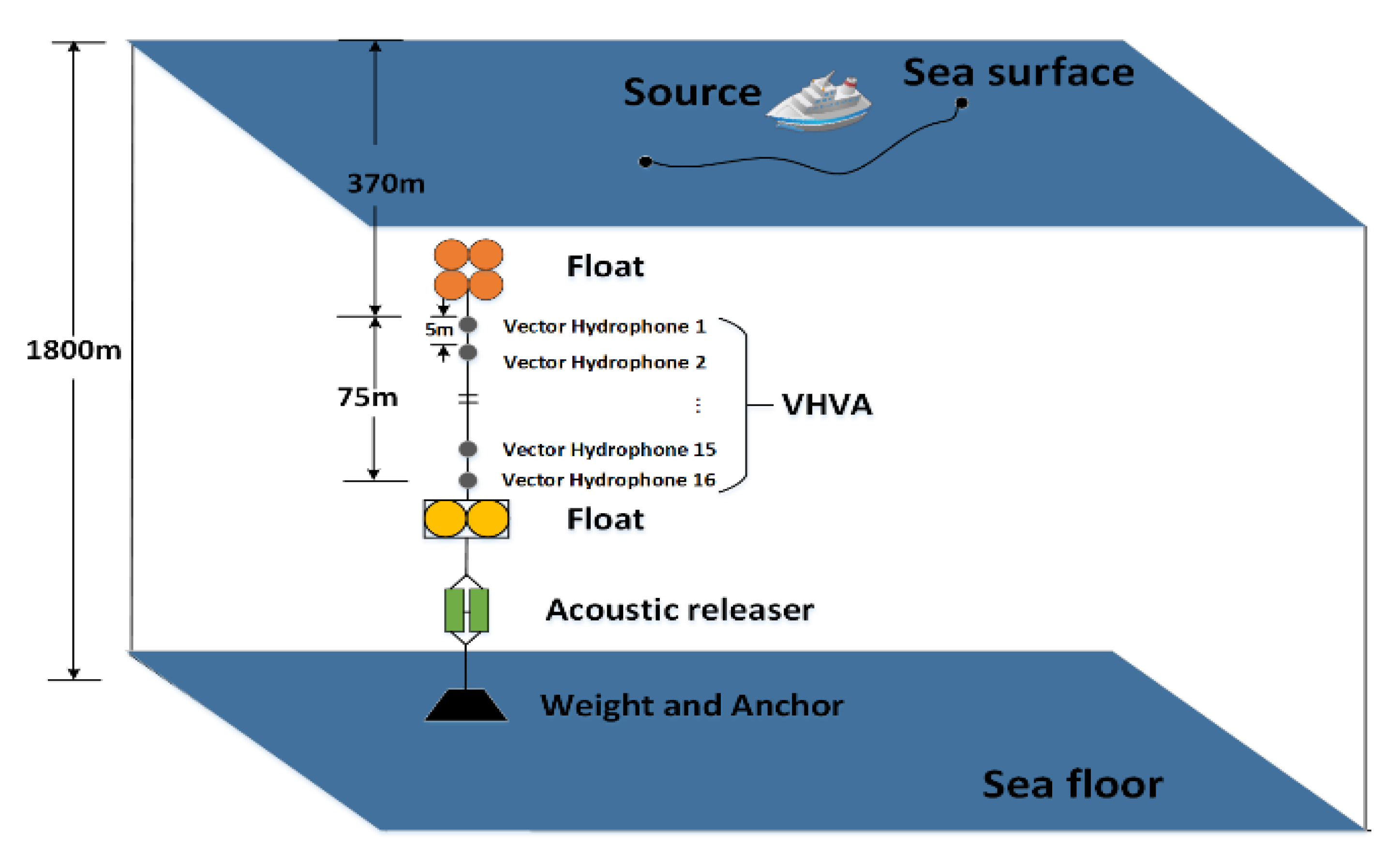
• The vertical hydrophone line array was composed of 16 elements with an interval of 5 m. The depth of the top hydrophone was 370 m, and that of the bottom sensor was about 445 m. The depth of water over the experimental area was about 1800 m.
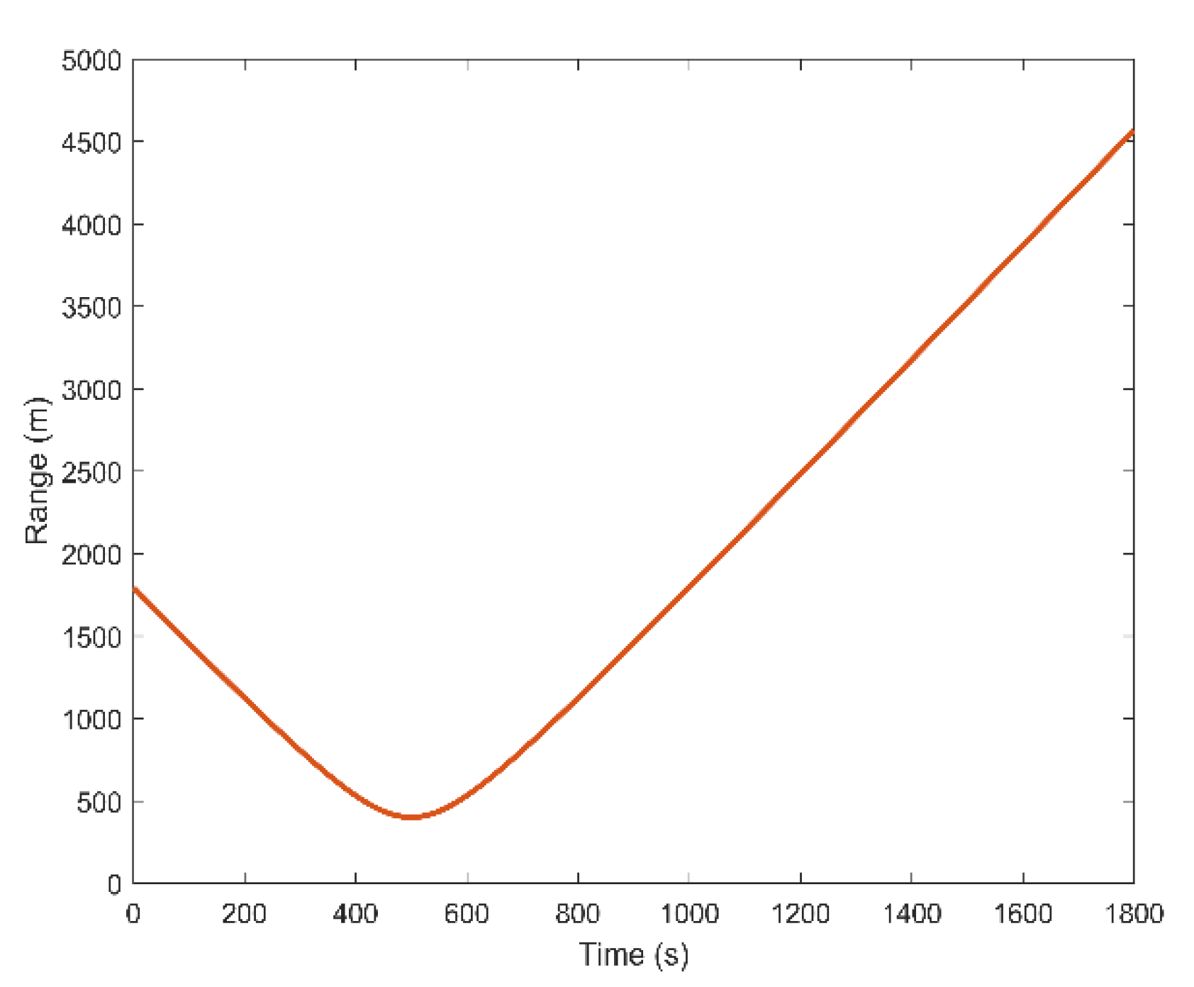
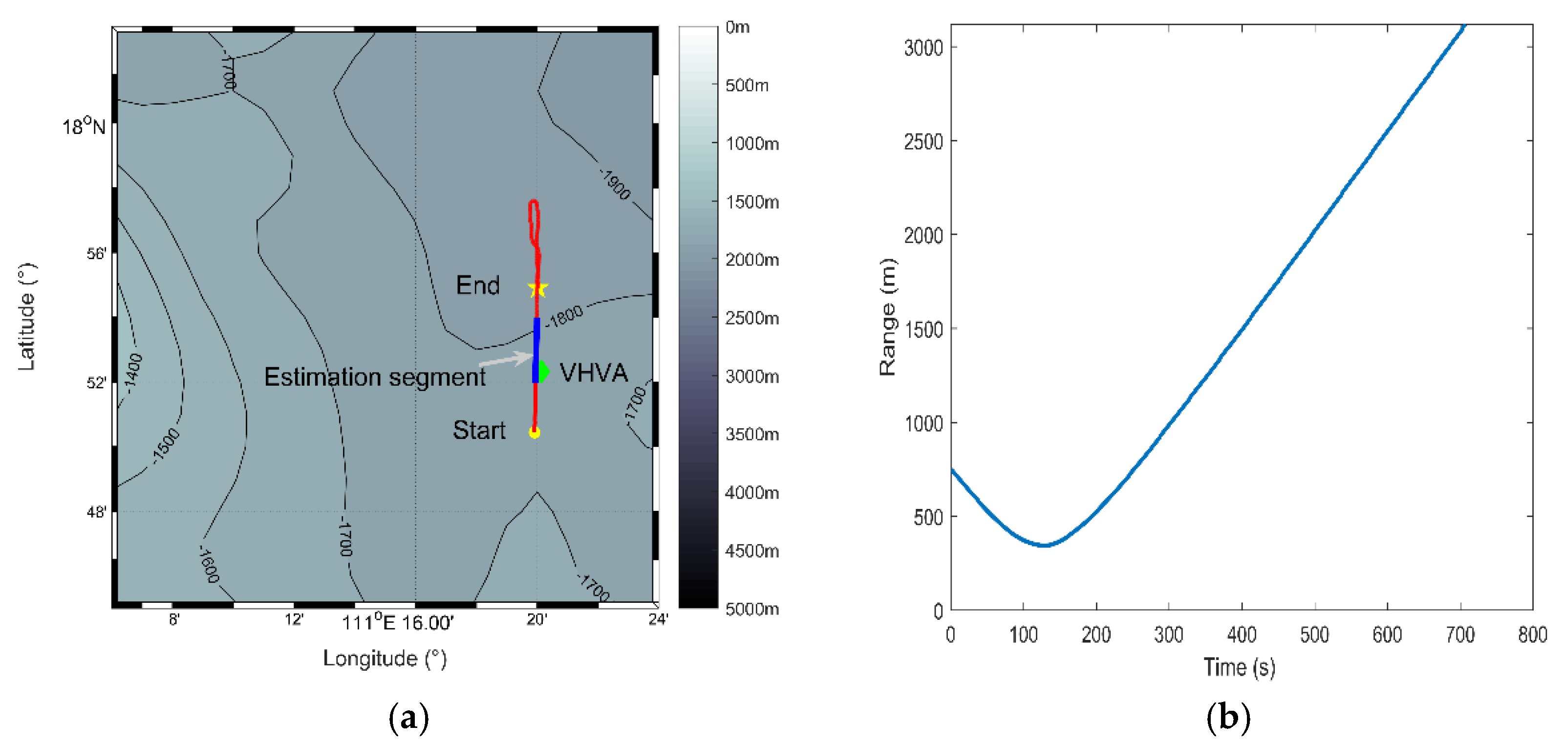
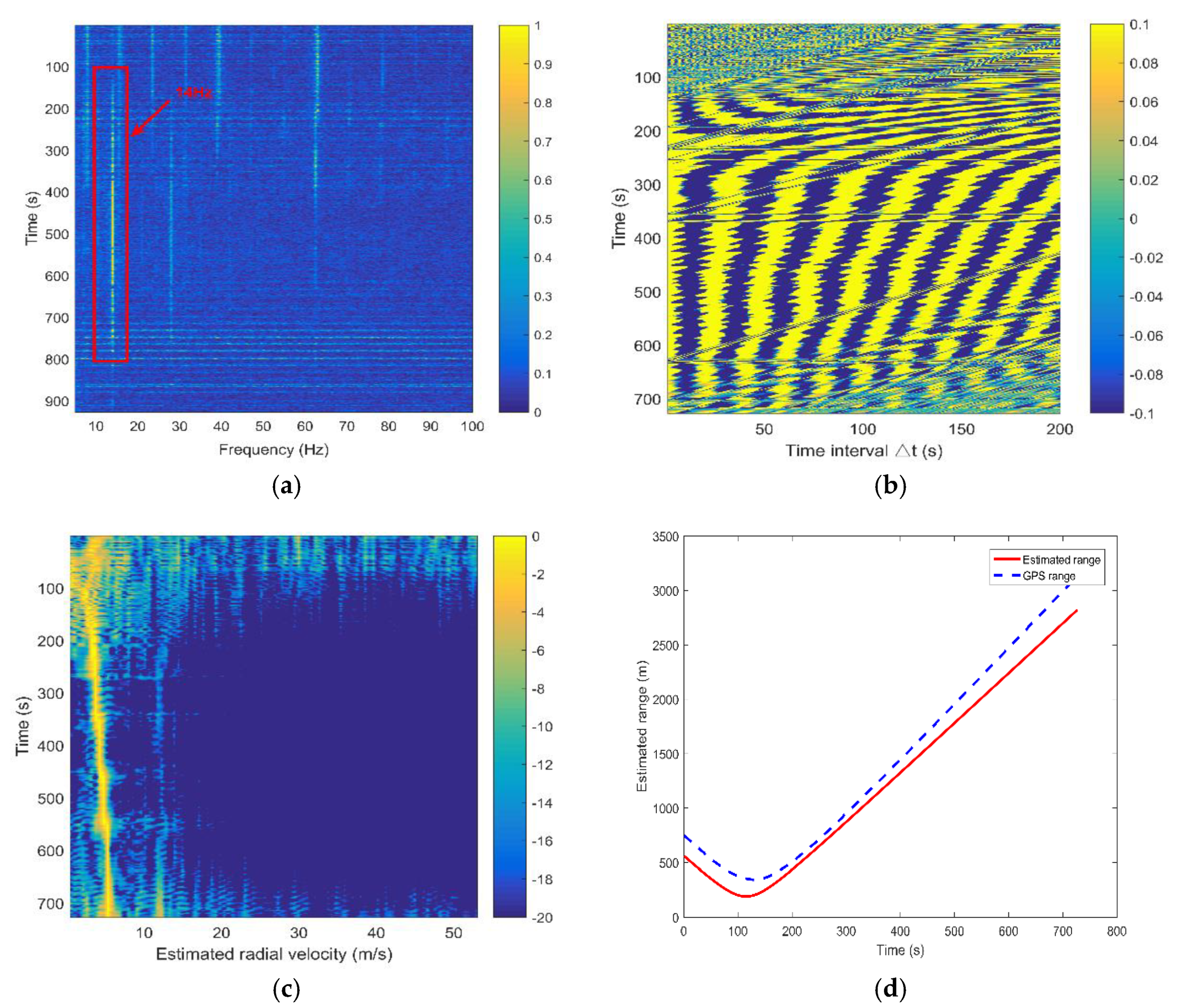
• The position where the heavy block attached below the array finally entered the water was regarded as the real array position recorded by the Global Positioning System (GPS) during the experiment. The moving vessel had GPS modules to record its real-time spatial positions. The corresponding trajectory map has been shown in Figure 10a. The real range from the ship to the array was calculated by GPS data and was then shown in Figure 10b. From this figure, we can see that the range and time of the CPA point were 344 m and 130 s, respectively. The moving velocity of the ship was about 5 m/s.
• The array may have a small tilt due to the disturbance of ocean currents. However, this small angular offset has little effect (only within 10%) on the final ranging result.
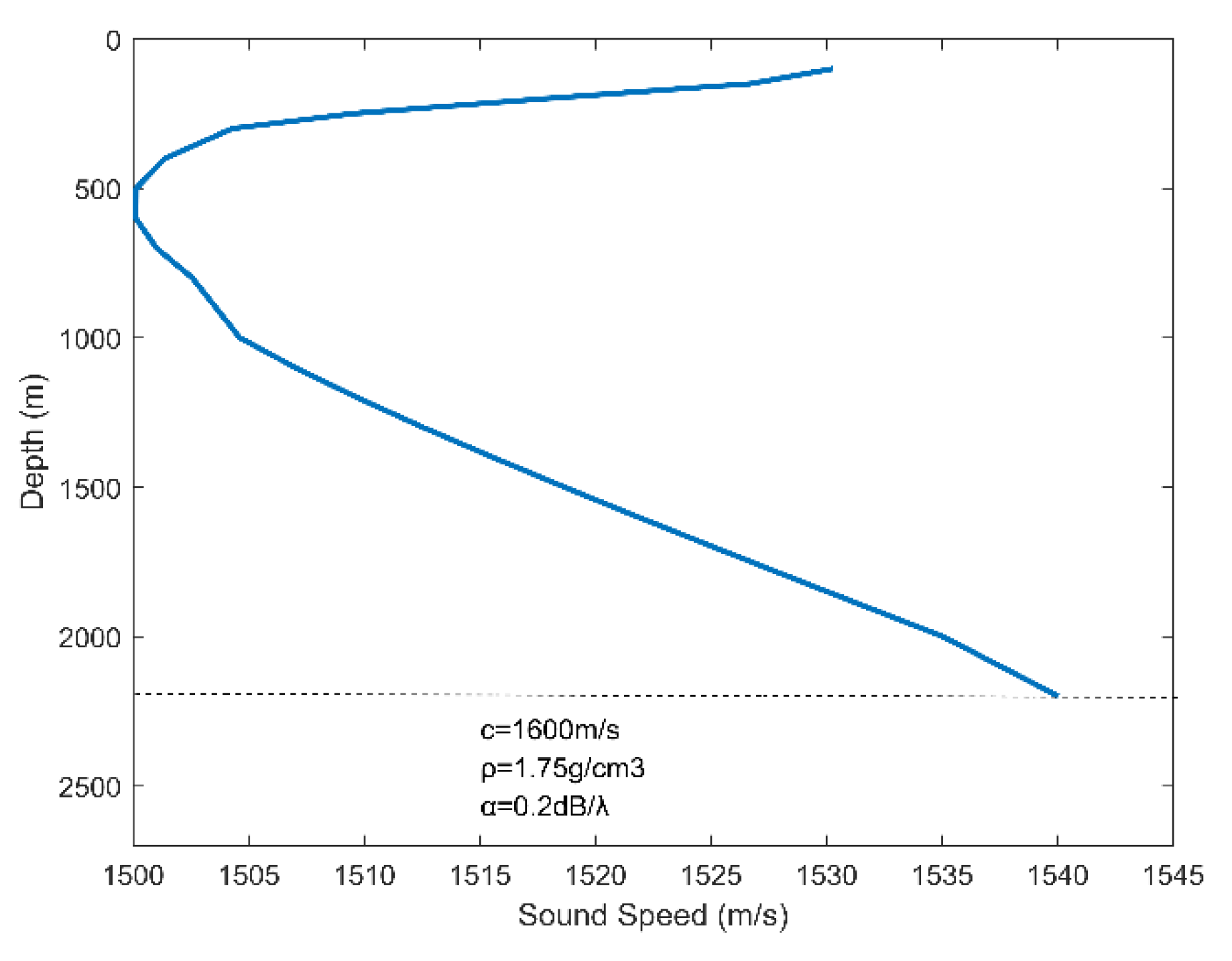
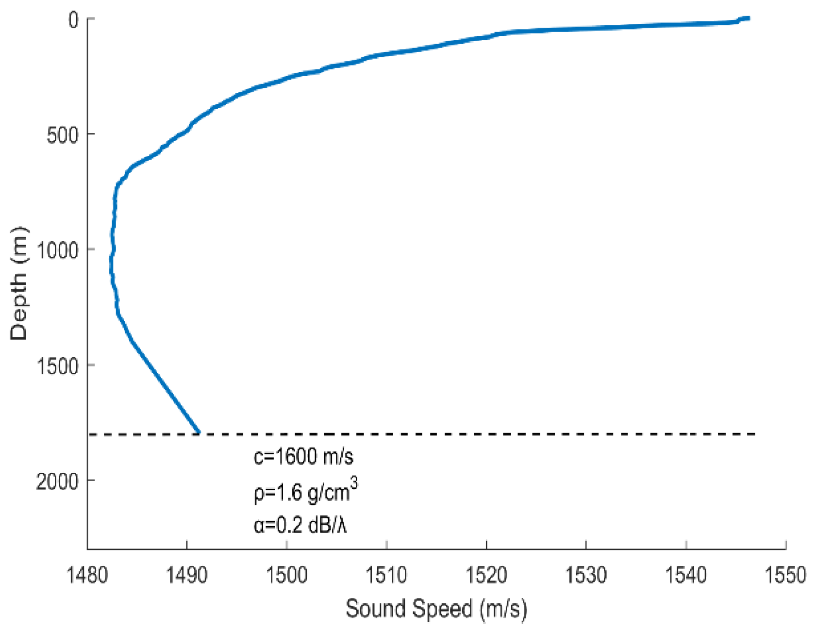
• The sound velocity profiler (SVP) was used to measure the sound speed profile (SSP) at the beginning of the experiments. The measured SSP is shown in Figure 11.
• The sampling rate was 16 kHz. The sea condition was level 3, and no other vessels passed during the measurement time.

4.2. Results Analysis

The top hydrophone is chosen as the reference element for the below discussion, and the other 15 elements are processed in the same way. Then, the range estimation results of 16 hydrophones are fused to improve the estimation accuracy. We choose a piece of data with a length of 900 s for processing. Figure 12 shows the time domain diagram and time-frequency domain diagram of the received signal for the reference element.

From Figure 12a, we can see that the received signal has a low-frequency envelope. Figure 12b validates that the ship-radiated noise contains multiple frequency components. In addition, adjacent spectrum components are prone to aliasing, and the low-frequency line spectrum components directly extracted from the spectrum are unstable. Therefore, the DEMON spectrum analysis method is employed to extract the stable low-frequency line spectrum. As shown in Figure 13a, the signal frequency after the DEMON analysis is 14 Hz.

The time interval between two points ranges from 1 s to 200 s, and the corresponding interference fringes of the sound intensity of the pressure difference is shown in Figure 13b. The period of the interference oscillations is calculated through Fourier transform and is then applied to calculate the radial velocity. The estimated radial velocity changing over time is shown in Figure 13c. From this figure, we can find that the estimated radial velocity is about 4.6 m/s. Then, when the MSE between the estimated value and true value reaches the minimum, the corresponding range and time of the CPA point can be obtained. Through the above processing, the range and time of the CPA point are 190 m and 115 s, respectively. Based on the above analysis, the range versus time is estimated by Equation (17). Then, the estimated range and the range recorded by the GPS data are compared in Figure 13d. The two curves have similar trends, but there is a slight difference in the range $r$ at the same time $t$. One can see that the range estimation result of a single hydrophone is inaccurate. Our experiment adopts a 16-element vertical hydrophone line array, and all of the elements are processed separately by the proposed method. Figure 14 shows the range estimation results of the 16 elements and the data fusion result.

From this figure, we can see that the estimation results of most elements are close to the GPS true value and that there are three obvious curves with large deviations. When performing WLS fusion, we assign smaller weights to the estimation results with larger range deviations, and larger weights to the elements with smaller deviations. Therefore, the fusion result is in good agreement with the actual curve.

To further measure the performance of this range localization method, we calculate the parameter of the relative mean square error (RMSE), defining RMSE as:

$${\sigma }_i{}^2={\displaystyle \sum _{j=1}^M{\left(\frac{r_i\left(t_j\right)-R\left(t_j\right)}{R\left(t_j\right)}\right)}^2 } i=1,2\cdots N$$

(28)

where $r_i\left(t_j\right)$ represents the estimated range at the $j$-th second by the $i$-th element. $R\left(t_j\right)$ is the real range at the $j$-th second. ${\sigma }_i{}^2$ is the RMSE of the $i$-th element. $M$ and $N$ are the length of time and the total number of elements. In this paper, we are more concerned about the accuracy of the estimation results near the CPA point, because the range, time and radial velocity of the CPA point determine the total estimated range. Therefore, we choose the estimation results of the first 300 s of Figure 14 for statistical calculations.

Table 1. RMSE of each element and the RMSE after fusion.

Element Number	#1	#2	#3	#4	#5	#6	#7	#8	#9
RMSE	0.0431	0.0208	0.0188	0.0212	0.0199	0.0225	0.1070	0.0393	0.0150
Element Number	#10	#11	#12	#13	#14	#15	#16	DF
RMSE	0.1209	0.0012	8.4 × 10 −4	1.8572	0.0553	1.2 × 10 −5	1.7 × 10 −4	4.9 × 10 −4

gives the RMSE of each hydrophone and the RMSE after the 16-element fusion.

From this table, we can see that the RMSEs of the 16 elements are slightly different. The RMSEs of the 7th, 10th and 13th element are significantly higher than those of the other elements, which is consistent with the curves in Figure 14. Moreover, the RMSE of the fusion results is 4.9 × 10⁻⁴, which is lower than the RMSE of most elements. Hydrophones at different depths receive signals with different SNRs. Inaccurate range estimation results can be obtained by a low SNR signal, as shown in the 7th, 10th and 13th element, because the sound signals at different depths go through different paths, undergoing different reflections and scattering. The signals reaching the receivers are attenuated differently, and the SNRs are also various.

The performance evaluation of the algorithm proposed in our paper is based on a comparison with real GPS data and the range estimation results obtained by a single hydrophone element. The comparison of these three results infer that this method can improve the estimation accuracy effectively and obtain a more accurate range estimation result than a single hydrophone.

It should be noted that the target and array should avoid being located in the shadow zone. In the shadow zone, the sound field is mainly composed of bottom-reflected rays rather than direct rays. The sound rays reflected by the sea bottom are greatly attenuated, and the SNRs of the signal received by the hydrophones are low. Thus, the range localization performance may be inaccurate.

5. Conclusions

In this paper, we proposed an algorithm to estimate the range of a moving ship. First, the DEMON spectrum analysis method is adopted to extract the low-frequency line spectrum components. Based on the sound intensity of the pressure difference, the extracted single-frequency signal at the given time interval interferes and forms the interference fringes in the plane of time and time interval. Then, the radial velocity of the moving source is derived from the period of interference oscillations. By fitting the time, velocity and range of the CPA point, we estimate the range from the source to the receiving hydrophone over time. Finally, range estimation results of multiple elements of the vertical line array are fused to obtain a more accurate estimation result. The simulation and deep-sea experiment analysis all verify that this method can estimate the range effectively. Moreover, the estimation accuracy is significantly improved since it fuses all the estimation results of each element and eliminates the impact of inaccurate results. The relative mean square error of the fusion result is lower than that of most hydrophones. In addition, this method does not require prior knowledge of marine environmental parameters and sound field modelling and thus demonstrates good universality. This method provides a new idea for the passive ranging of moving ships.

References

- Mei, J.D.; Hui, J.Y.; Hui, J. Research on simulation of near field passive ranging with underwater acoustic image by focused beam-forming. J. Syst. Simul. 2008, 20, 1328–1333. [Google Scholar]
- Peng, C.; Jiang, K.Y. Research on passive ranging of three-element correlation. Tech. Acoust. 2012, 31, 431–435. [Google Scholar]
- Baggeroer, A.B.; Kuperman, W.A. Matched field processing: Source localization in correlated noise as an optimum parameter estimation problem. J. Acoust. Soc. Am. 1988, 83, 571–587. [Google Scholar] [CrossRef]
- Tollefsen, D.; Dosso, S.E. Matched-field source localization with multiple small-aperture arrays. J. Acoust. Soc. Am. 2015, 138, 1754. [Google Scholar] [CrossRef]
- Tollefsen, D.; Dosso, S.E. Source localization with multiple hydrophone arrays via matched-field processing. IEEE J. Ocean. Eng. 2016, 42, 654–662. [Google Scholar] [CrossRef]
- Cockrell, K.L.; Schmidt, H. Robust passive range estimation using the waveguide invariant. J. Acoust. Soc. Am. 2010, 127, 2780. [Google Scholar] [CrossRef] [PubMed]
- Rakotonarivo, S.T.; Kuperman, W.A. Model-independent range localization of a moving source in shallow water. J. Acoust. Soc. Am. 2012, 132, 2218. [Google Scholar] [CrossRef] [PubMed]
- Rémi, E.; Julien, B.; Marie, G.; Xavier, C.; Thierry, C. Understanding deep-water striation patterns and predicting the waveguide invariant as a distribution depending on range and depth. J. Acoust. Soc. Am. 2018, 143, 3444–3454. [Google Scholar]
- Young, A.H.; Harms, H.A.; Hickman, G.W.; Rogers, J.S.; Krolik, J.L. Waveguide-invariant-based ranging and receiver localization using tonal sources of opportunity. IEEE J. Ocean. Eng. 2019, 45, 631–644. [Google Scholar] [CrossRef]
- Li, J.; Sun, G.Q.; Han, Q.B.; Zhang, C.H. Acoustics Vector Sensor Linear Array Passive Ranging Based on Waveguide Invariant. J. Acoust. Soc. Am. 2012, 1495, 576–586. [Google Scholar]
- Cho, C.; Song, H.C.; Hodgkiss, W.S. Robust source-range estimation using the array/waveguide invariant and a vertical array. J. Acoust. Soc. Am. 2016, 139, 63–69. [Google Scholar] [CrossRef] [PubMed]
- Cheng, Y.S.; Wang, Y.C.; Shi, G.Z.; Hui, J.Y. DEMON analysis of underwater target radiation noise based on modern signal processing. Tech. Acoust. 2006, 25, 71. [Google Scholar]
- Chung, K.W.; Sutin, A.; Sedunov, A.; Bruno, M. DEMON acoustic ship signature measurements in an urban harbor. Adv. Acoust. Vib. 2011, 2011. [Google Scholar] [CrossRef]
- Yao, Z.X.; Hui, J.Y.; Wang, D.J.; Cai, P. Identifying two targets by a single vector hydrophone based on the DEMON spectrum. Appl. Acoust. 2005, 3, 171–176. [Google Scholar]
- Klein, L.A. Sensor and Data Fusion Concepts and Applications; Society of Photo-Optical Instrumentation Engineers (SPIE) Press: Bellingham, WA, USA, 1999. [Google Scholar]
- Li, X.; Ma, X. Underwater data fusion of multiple arrays in a mono-platform for low SNR. In Proceedings of the 2017 IEEE International Conference on Signal Processing, Xiamen, China, 22–25 October 2017; pp. 1–4. [Google Scholar]
- Dos Santos, M.M.; De Giacomo, G.G.; Drews, P.L.J.; Botelho, S.S.C. Underwater sonar and aerial images data fusion for robot localization. In Proceedings of the 2019 19th International Conference on Advanced Robotics (ICAR), Belo Horizonte, Brazil, 2–6 December 2019; pp. 578–583. [Google Scholar]
- Yan, J.; Xu, Z.Q.; Luo, X.Y.; Chen, C.L.; Guan, X.P. Feedback-based target localization in underwater sensor networks: A multi-sensor fusion approach. IEEE Trans. Signal Inf. Process. Over Netw. 2018, 5, 1. [Google Scholar] [CrossRef]
- Prasanna, K.L.; Rao, S.K.; Jagan, B.O.L.; Jawahar, A.; Karishma, S.B. Data fusion in underwater environment. Int. J. Eng. Technol. 2016, 8, 225–234. [Google Scholar]
- Jensen, F.B.; Kuperman, W.A.; Porter, M.B.; Schmidt, H. Computational Ocean. Acoustics; Springer: New York, NY, USA, 2011; pp. 338–340. [Google Scholar]
- Liang, Y.; Meng, Z.; Chen, Y.; Zhang, Y.; Wang, M.; Zhou, X. A data fusion orientation algorithm based on the weighted histogram statistics for vector hydrophone vertical array. Sensors 2020, 20, 5619. [Google Scholar] [CrossRef] [PubMed]