Article

Antenna/Body Coupling in the Near-Field at 60 GHz: Impact on the Absorbed Power Density

IETR (Institut d’Électronique et des Technologies du Numérique), French National Center for Scientific Research (CNRS), University of Rennes-UMR 6164, F-35000 Rennes, France
*
Author to whom correspondence should be addressed.
Appl. Sci. 2020, 10(21), 7392; https://doi.org/10.3390/app10217392
Submission received: 24 September 2020 / Revised: 15 October 2020 / Accepted: 18 October 2020 / Published: 22 October 2020
(This article belongs to the Special Issue Human Exposure in 5G and 6G Scenarios)

Abstract

:
Wireless devices, such as smartphones, tablets, and laptops, are intended to be used in the vicinity of the human body. When an antenna is placed close to a lossy medium, near-field interactions may modify the electromagnetic field distribution. Here, we analyze analytically and numerically the impact of antenna/human body interactions on the transmitted power density (TPD) at 60 GHz using a skin-equivalent model. To this end, several scenarios of increasing complexity are considered: plane-wave illumination, equivalent source, and patch antenna arrays. Our results demonstrate that, for all considered scenarios, the presence of the body in the vicinity of a source results in an increase in the average TPD. The local TPD enhancement due to the body presence close to a patch antenna array reaches 95.5% for an adult (dry skin). The variations are higher for wet skin (up to 98.25%) and for children (up to 103.3%). Both absolute value and spatial distribution of TPD are altered by the antenna/body coupling. These results suggest that the exact distribution of TPD cannot be retrieved from measurements of the incident power density in free-space in absence of the body. Therefore, for accurate measurements of the absorbed and epithelial power density (metrics used as the main dosimetric quantities at frequencies > 6 GHz), it is important to perform measurements under conditions where the wireless device under test is perturbed in the same way as by the presence of the human body in realistic use case scenarios.

1. Introduction

The increasing need for high data rate mobile communications, mainly driven by video streaming and cloud computing, has led to fast development of heterogeneous fifth-generation (5G) cellular mobile networks expected to exploit the lower part of the millimeter-wave (mmW) band. In particular, the 60-GHz band has been identified as an attractive solution for radio access and backhauling in the future mmW systems [1]. The deployment of mmW small cells will allow for larger channel bandwidth, higher data rates, secure short-range communications, low interference with adjacent cells, and compact systems [2,3,4,5].
Wireless devices, such as mobile phones, tablets, and laptops are intended to be used in the vicinity of the human body (e.g., phone call or browsing scenarios), and they should comply with the exposure limits. Below 6 GHz, the specific absorption rate (SAR) is used as the main dosimetric quantity [6,7]. In the 6–300 GHz range, the electromagnetic energy is deposited predominantly in superficial tissues (the penetration depth is approximately 0.5 mm at 60 GHz [8,9,10,11]). As a consequence, the International Commission on Non-Ionizing Radiation Protection (ICNIRP) and the Institute of Electrical and Electronics Engineering (IEEE) recommend, respectively, the absorbed power density and epithelial power density as the main dosimetric quantities. Both the ICNIRP and IEEE set the limits to 10 mW / cm 2 for occupational environments (referred to as restricted environments in the IEEE standard), and 2 mW / cm 2 for the general public (referred to as unrestricted environments in the IEEE standard). Above 6 GHz, the power density is to be averaged over 4 cm 2 and 6 min. Moreover, from 30 to 300 GHz, the power density is to be averaged over 1 cm 2 and must not exceed two times the exposure limit for 4 cm 2 . The existing dosimetry systems [12,13,14] are designed to measure the incident power density in free space close to a wireless device under test. In [12], the incident power density is obtained from the measurement of the magnitude and polarization of the E-field, whereas in [13] it is determined from the measurement of both the E- and H-field using the two-probe method. Both [12] and [13] use field probes from 6 to 110 GHz allowing for measurements down to 2 mm and 0.5 mm from the device under test, respectively. The system presented in [14] uses a multi-probe technology combined with switching networks for spherical near-field measurements in the 18–50 GHz range to retrieve the incident power density. When an antenna is placed in the vicinity of a lossy medium, such as human skin, electromagnetic contrast at the air/skin interface results in the appearance of scattered field and near field interactions, which modify the field impinging the human body compared to the free-space radiation [15,16]. Hence, in free-space measurements of the incident power density, variations of the power density due to the coupling of a wireless device with the human body are not taken into account. This coupling may impact the power absorption in the human body as well as resulting heating [17].
Various aspects related to the interactions of mmWs with the human body have been reviewed in the literature. The study performed in [18] for a terminal with a 60-GHz antenna module for several representative human body exposure scenarios, showed that both hand and head, located in the antenna near-field region, significantly affect the antenna reflection coefficient, radiation pattern, and efficiency. The alteration of the antenna radiation characteristics by the human body in the near-field may therefore affect the total field impinging the body. At lower microwave frequencies (i.e., 900 and 1900 MHz), studies performed to assess the influence of the source/phantom interactions on the transmitted field, demonstrated that the electric field may be significantly modified depending on the position of the antenna in respect to the phantom (decrease down to 25% and enhancement up to two times of the electric field amplitude at 900-MHz for a dipole and mobile terminal, respectively) [15,16]. On the other hand, a study conducted mainly at 24 GHz, with some results at 60 GHz, showed that the source/body interaction is relatively weak (enhancement by 10% of the squared E-field for a dipole array with four elements at 60 GHz) [19]; however, only electrically small antennas were investigated in that study. The impact on the transmitted to the body field is expected to be higher for wireless devices equipped with larger antennas (e.g., patch antenna arrays).
The main purpose of this study is to analyze the impact of the antenna/human body interactions in the near-field on the transmitted power density (TPD) at 60 GHz. For the first time, the fundamental limits in terms of enhancement and decrease in the TPD are investigated. Sources of increasing complexity are compared, including plane waves with and without free-space losses, antenna-equivalent sources, and patch antenna arrays. For antenna arrays, the role of the directivity and ground plane dimensions are also investigated.

2. Materials and Methods

We define here the exposure scenarios considered in this study. Then, the analytical and numerical methods used for exposure assessment are presented.

2.1. Exposure Scenarios

To analyze variations of TPD in the skin-equivalent model due to the presence of a radiating structure, seven scenarios of increasing complexity are considered (Figure 1). Scenarios 1–4 are considered to determine the fundamental limits of TPD variations for a plane-wave excitation. In scenarios 5 and 6, we model the radiation pattern of antennas neglecting the impact of the phantom and a perfect electric conductor (PEC) on the antenna performances. Finally, antennas placed close to the skin-equivalent model are considered in scenario 7. These scenarios are detailed hereafter.
  • Scenario 1: Plane-wave incident from free space onto a semi-infinite flat skin-equivalent model (Figure 1a).
Normal incidence is considered to represent the worst-case exposure scenario with maximum TPD [20]. Due to a shallow penetration depth at mmWs (<1 mm), the interaction with the human body is mainly limited to skin. As a consequence, a homogenous skin-equivalent layer is used as a model [21,22]. The dielectric properties of skin-equivalent model are those of dry skin at 60 GHz ( ε = 7.98 j 10.90 ); they were extracted from [23]. For completeness, we also provide in the paper the main results for a wet skin model ( ε = 10.22 j 11.83 [23]).
  • Scenario 2: Scenario 1 adding a perfect electric conductor (PEC) parallel to the skin model (Figure 1b).
The total transmitted field ( E Total , TPD Total ) is equal to the superposition of the transmitted field from direct incidence ( E Direct , TPD Direct ) and the scattered field resulting from multiple reflections at the PEC/skin-model interface es ( E R , TPD R ).
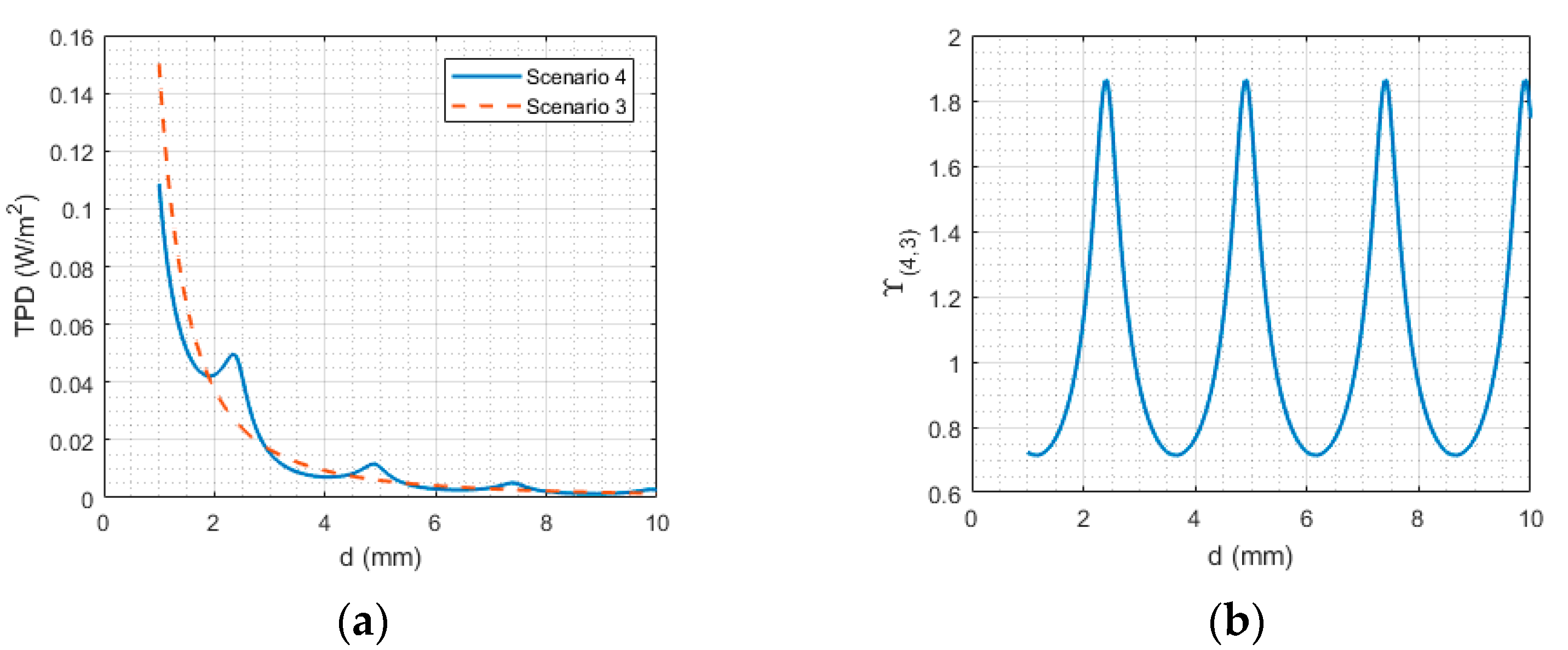
  • Scenario 3: Scenario 1 with free-space losses (i.e., the amplitude of the plane-wave is attenuated in free space) (Figure 1c).
The amplitude of the electric field radiated by an infinitesimal dipole decreases as 1/d in the far-field, where d is the distance between the source and the observation point. Hence, we assume in this scenario that the amplitude of the incident E-field decreases with an attenuation function f(d)   = 1 / d .
  • Scenario 4: Scenario 2 with free-space losses (Figure 1d).
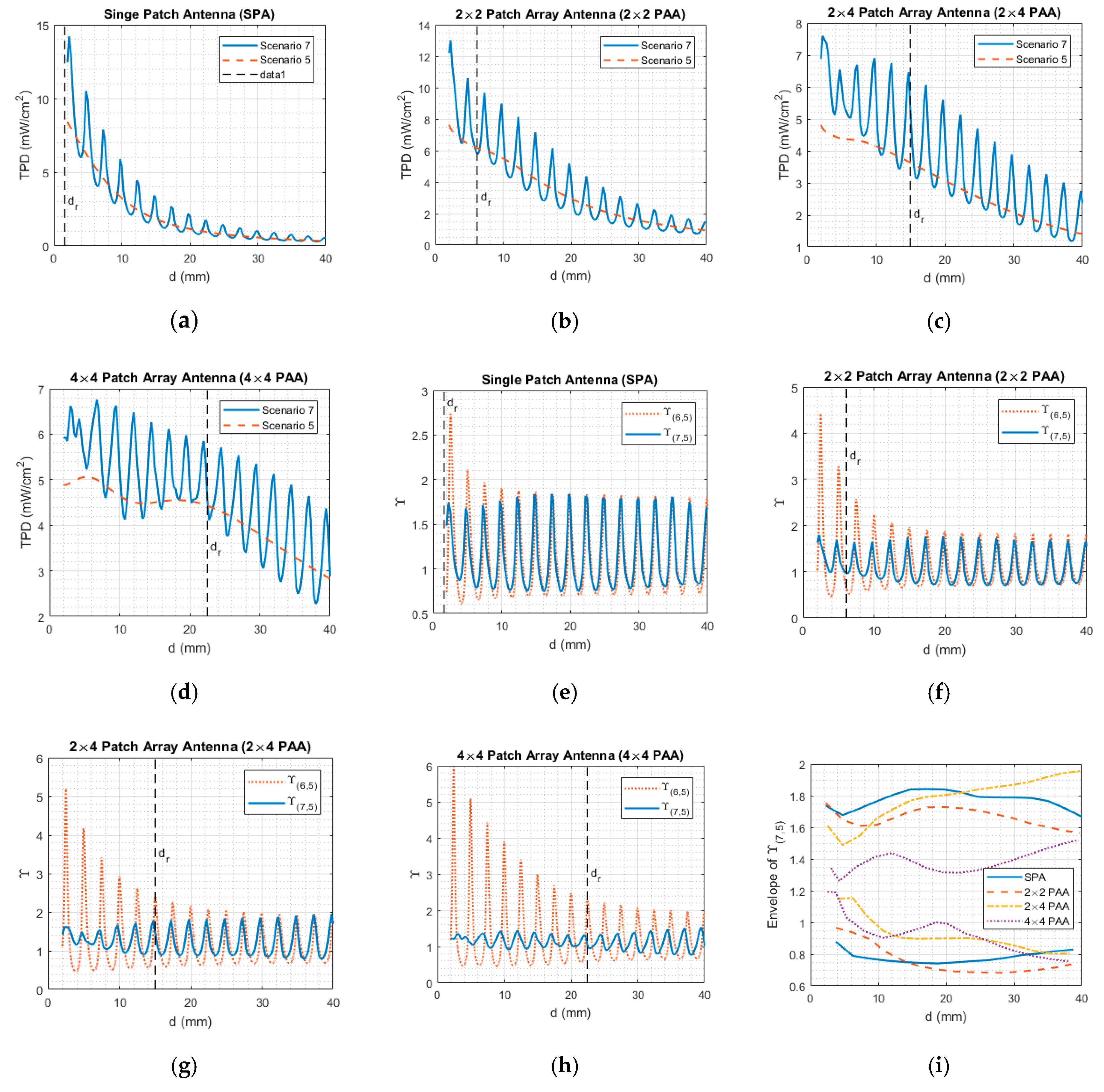
  • Scenario 5: Scenario 1 with an antenna equivalent source replacing the plane-wave illumination (Figure 1e).
The antenna equivalent source is defined as a combination of equivalent electric and magnetic currents flowing on a closed surface surrounding the antenna (dashed line in Figure 1e) generating the same electromagnetic field as the antenna in free space.
  • Scenario 6: Scenario 2 with the antenna equivalent source replacing the plane-wave illumination (Figure 1f).
  • Scenario 7: Realistic antennas placed in the vicinity of the skin model (Figure 1g).
The source main beam is directed towards the phantom representing the worst-case exposure scenario. Several sources have been considered: single patch antenna (SPA) and patch antenna array (PAA) with 4, 8, or 16 (2 × 2 PAA, 2 × 4 PAA, and 4 × 4 PAA, respectively) radiating elements, inspired from [10,24] (Figure 2 and Figure 3) and matched to 50 Ω in free-space at 60 GHz. All results are provided for an antenna input power of 10 mW.

2.2. Analytical Method: Plane Wave Illumination

The problem of a normally-incident plane wave (scenarios 1–4) at a planar interface between free space and a lossy region representing skin was solved analytically in [25]. Without loss, the electric field is given by:
E i n c = E 0 e jk 0 d   x ^   ,
where E 0 is the amplitude of the electric field, k 0 is the free space wavenumber, and d is the normal distance between the plane-wave source and skin model interface. Assuming that the plane wave is attenuated in free space, its E-field vector is given by:
E i n c = E 0 e jk 0 d f ( d )   x ^   ,  
where f(d) is an attenuation function. The transmitted E-field vector ( E tr ) at the phantom interface is therefore expressed as [25] (Appendix A):
Scenario 1 :
E tr = T 1 E inc   ,  
Scenario 2:
E tr = T 1   1 1 + e j 2 dk 0 R 1 E inc   ,
Scenario 3:
E tr = T 1 E inc   ,
Scenario 4:
E tr = T 1 E i n c + T 1 E 0 e jdk 0 n = 1 ( e j 2 dk 0 R 1 ) n f ( ( 2 n + 1 ) d ) x ^   ,  
where T 1 and R 1 are the transmission and reflection coefficients, respectively, calculated using Fresnel coefficients at the free space/skin model interface [25]. The TPD for a plane-wave can be computed as:
TPD = Re [ | E tr | 2 η ]     ,
where η is the complex intrinsic impedance of the skin.

2.3. Analytical Method: Equivalent Source

For scenarios 5 and 6, the electric field was modeled analytically using the plane-wave spectrum theory [26,27,28]. It represents the spatial distribution of each field component over a transverse plane as a superposition of the plane waves propagating along different directions defined by the couplet   K = k x x ^ + k y y ^ , also called the plane wave spectrum (PWS). The PWS of an electric field phasor component E ( R , z 0 ) over a plane Ψ identified by z = z 0 and   R = x x ^ + y y ^ is expressed as:
E ^ ( K , z 0 ) =   R E ( R , z 0 ) e j K · R d R   .
The strength of this approach is its ability to represent the propagation of a complex field topography through space. The PWS over any plane parallel to Ψ located at distance l in a homogenous medium is computed by multiplying the PWS at z = z 0 by the propagator P ( K , l ) = e jk z l :
E ^ ( K , z 0 + l ) = E ^ ( K , z 0 )   P ( K , l )   ,
where k z is the longitudinal propagation constant given as k z = k 2 | K | 2 , k is the propagation constant.
For exposure scenario 5, the tangential spectrum components of the incident and transmitted fields at the air/phantom interface are related as:
E ^ tr | | ( K ) = Π 1 E ^ i n c | | ( K )   ,
where Π 1 is the spectral transmission operator given in [26]. The normal field spectrum component is obtained from the tangential field spectra E ^ | | using the Gauss law:
E ^ z = K · E ^ | | k z   .
For exposure case 6, the total transmitted field spectrum is given as (refer to Appendix A for more details):
E ^ tr | | ( K ) = Π 1 ( I + P ( K , 2 d ) Γ 1 ) 1 E ^ i n c | | ( K )   ,
where I is the identity matrix, d is the PEC–phantom separation distance, Γ 1 is the spectral reflection coefficients at the phantom interface given in [26]. The H-field spectrum is calculated as [28]:
H ^ tr ( m ) = 1 μ ω ( k ) × ( E ^ tr )   .
The spatial field components ( E and H ) are retrieved using the inverse Fourier transform of the field spectra. The TPD is calculated as [6]:
TPD = A Re [ E × H * ] · d s A   ,
where ds is the integral variable vector with the normal direction to the integral area A on the body surface. All results are provided for an averaging area A of 1   cm 2 (except 2-dimensinoal TPD distributions provided in Section 3.2 and Section 3.3). Note that the TPD is identical to the absorbed power density as defined in [6] and to the epithelial power density as defined by [7].

2.4. Numerical Method: Patch Antenna Arrays

Scenario 7 was analyzed numerically using the finite integration technique (FIT) implemented in CST Studio Suite 2019. The convergence is reached by setting a finer mesh around the air/phantom interface (i.e., 1 μm) and larger beyond (i.e., 0.356 mm corresponding to λ g /50, where λ g is the guided wavelength in the phantom). Open boundaries are used representing the free-space conditions (i.e., no reflected field at the boundaries of the computational volume). The number of mesh cells varies from 26 to 80 million with the antenna/phantom separation distance. Typical duration of single simulation varies from 35 to 75 min using high-performance workstations with accelerators (Xeon Gold 6140, 768 Go RAM, NVIDIA Quadro GV100; Dell, TX, USA).

3. Results

To analyze the TPD variations due to the antenna/body coupling, the following figure of merit is defined:
Υ ( m , n ) = TPD m TPD n   ,
where TPD m and TPD n are the TPD from exposure scenarios m and n, respectively, with m     { 2 ,   4 ,   6 ,   7 } and n     { 1 ,   3 ,   5 } . In practice, the separation distance between a wireless device and its user may vary. To account for this variation during exposure, we also calculated the floating average Υ ¯ ( m , n ) over the range of distances Δ d   { 1 ,   3 ,   5 }   mm .

3.1. Fundamental Limits: Plane-Wave Illumination

First, we assess the TPD changes due to presence of a PEC layer in front of the skin model for plane-wave illumination (scenarios 1 and 2). To this end, TPD 1 , TPD 2 , and Υ ( 2 , 1 ) are calculated using (3), (4), (7), and (15) for E 0 = 10   V / m and R 1 = 0.59 + j 0.16 (Figure 4).
Figure 4 shows that the TPD at the surface of the phantom is strongly altered by the presence of PEC (increase up to 574% and decrease down to 61.7%). Υ ( 2 , 1 ) can be expressed as:
Υ ( 2 , 1 ) = TPD 2 TPD 1 = | T 1 1 1 + e j 2 dk 0 R 1 E inc | 2 | T 1 E inc | 2 = | 1 1 + e j 2 dk 0 R 1 | 2 .
The positions of Υ ( 2 , 1 ) maxima and minima ( d max Υ ( 2 , 1 ) and d min Υ ( 2 , 1 ) ) depend on the phase of R 1 and given by:
d min Υ ( 21 ) = R 1 π + π n   2 k 0   ,
d max Υ ( 21 ) = R 1 π + 2 π n   2 k 0   ,
where n is an integer number, R 1 is the phase shift introduced by the phantom interface to the reflected plane-wave. The fundamental limits of Υ ( 2 , 1 ) can be found by replacing (17) and (18) in (16):
1 | 1 + | R 1 | | 2 Υ ( 2 , 1 ) 1 | 1 | R 1 | | 2   .
Equation (19) shows that the higher the magnitude of the phantom reflection coefficient, the higher the TPD variations. For example, for a wet skin model, the variations of TPD are more pronounced (increase up to 629% and decrease down to 62.3%, respectively). Note that these variations are also age-dependent as the tissue properties evolve with age [29]. In particular, for 5 year old children the enhancement increases to 640%. For the sake of brevity, in the rest of the paper, the analysis for wet skin and age-dependent effects will be omitted (except Section 3.3). Table 1 provides the maximum and minimum Υ ¯ ( m , n ) . The results show that the average TPD increases due to the presence of PEC (roughly a 60% increase for Δ d = 5   mm ).
Next, the free-space losses are taken into account in the analysis (scenarios 3 and 4). TPD 3 , TPD 4 , and Υ ( 4 , 3 ) are calculated using (5), (6), (7), and (15) (Figure 5).
TPD 4 demonstrates a damped oscillatory behavior around TPD 3 (increase up to 80% and decrease down to 28%). Due to the free-space loss, the oscillation amplitude of Υ ( 4 , 3 ) is lower compared to Υ ( 2 , 1 ) . The averaged TPD over distance increases due to the presence of PEC (i.e., maximum increase of 41%, 15%, 5% for Δd = 1 mm, 3 mm, 5 mm, respectively) (Table 2).

3.2. Fundamental Limits: Equivalent Sources

Here, we consider the equivalent sources corresponding to the patch antenna arrays radiating in free space (Figure 2). This allows us to model the case where the free-space antenna matching, efficiency, and radiated field are preserved and not modified by the phantom (scenarios 5 and 6). TPD 5 , TPD 6 , and Υ ( 6 , 5 ) are calculated from Equations (8)–(15) (Figure 6a–e).
Significant differences in Υ ( 6 , 5 ) maxima and, to a smaller extent, minima between the antenna-equivalent sources are noted for d < 25 mm (Figure 6e). The TPD increases (decreases) up to (down to) 174% (39%), 342% (54%), 421% (54.7%), and 497% (54.7%) for the SPA, 2 × 2 PAA, 2 × 4 PAA, and 4 × 4 PAA, respectively. This is due to the differences in the attenuation rate of the peak power density in free-space PD fs   of the antenna-equivalent sources (Figure 6f). Indeed, when the PD fs attenuation rate is higher, Υ ( 6 , 5 ) is lower. At d = 35mm, Υ(6,5) of all antenna-equivalent sources converges to the same oscillatory function (with relative difference < 10%) (Figure 6e). Figure 7 shows that as d increases, Υ ( 6 , 5 ) converges to Υ ( 4 , 3 ) as the power density in free-space decreases as 1/ d 2 in the far-field. Maximum values of Υ ¯ ( 6 , 5 ) are obtained for 4 × 4 PAA (i.e., the maximum increase of 247%, 124%, 76% for Δd = 1mm, 3mm, 5mm, respectively) (Table 3). Note that for the antenna-equivalent sources max Υ ¯ is up to 2.5 times higher compared to the plane wave with free-space losses (compare Table 2 and Table 3).
To obtain a deeper insight into the TPD variations, we analyzed the changes in the spatial distribution of TPD for the SPA equivalent source due to the presence of PEC (Figure 8). The distribution of TPD 6 is affected by the presence of PEC and evolves with d. For d corresponding to the maximum TPD (i.e., 4.75 mm, 7.25 mm, 17.25 mm), the absorbed power density is concentrated around its maximum. It extends progressively over a larger surface when d approaches the value corresponding to TPD minima (i.e., 6.5 mm, 9.0 mm, 18.75 mm). When the spatial distribution of TPD is concentrated around its maxima, the spatial averaging area has a stronger impact on the mean TPD, which rapidly decreases with the averaging area (e.g., the ratio between TPD averaged over 1 cm 2 and 4 cm 2 equals to 3.26 and 1.86 for d = 4.75 and 6.5 mm, respectively).
The cross-section distributions along x-axis at y = 0   mm of the x component of E Direct , E Total , and E R are plotted in Figure 9. The amplitude of E Total is directly related to the phase difference between E Direct and E R . For d = 7.25 mm, E Direct   is in phase with E R around x = 0 mm. This null phase difference evolves periodically along the x-axis resulting in either constructive or destructive interferences. Consequently, this results in an enhancement of the E Total amplitude for x ∈ (−5.0; 5.0) mm and in a decrease for x ∈ (−10; −5) U (5; 10) mm, thus explaining the higher spatial gradient of TPD in Figure 8a,c,e (middle line, scenario 6). On the other hand, for d = 9.0 mm, E Direct and   E R are out of phase at x = 0 mm. This results in a decrease in the E Total for x = (−5.0; 5.0) mm and its enhancement for x = (−10; −5) U (5; 10) mm, resulting in spread of TPD in Figure 8b,d,f (middle line, scenario 6). Note that similar observations were made for the y and z components of the field (for the sake of brevity, the data are not shown).

3.3. Patch Antenna Arrays

When an antenna is located in the vicinity of a scatter, its matching and radiation are altered. To exclude the effect of the antenna mismatch, TPD 7 is normalized to (1- S 11 / Ph 2 ) and TPD 5 to (1- S 11 / FS 2 ), where S 11 / Ph and S 11 / FS are S 11 of the antenna in the presence of the phantom and in free space, respectively. Note that modern wireless devices are equipped with matching networks designed to compensate for the mismatch.
The changes in the TPD due to the antenna/phantom coupling (scenarios 5 and 7) are shown in Figure 10. For d < d r , where d r denotes the interface between the reactive and radiating near-field regions, the changes in term of the absolute value of TPD are more pronounced (Figure 10a–d). In terms of the relative variations, for this range of d, the TPD increases up to 79.2%, 71.6%, and 43.8% and decreases down to 4.4%, 9.75%, and 9.84% for 2 × 2 PAA, 2 × 4 PAA, and 4 × 4 PAA, respectively (Figure 10e–h). The results shown in Figure 10i demonstrate that there is no direct correlation between Υ ( 7 , 5 ) and the source directivity. Note that Υ ( 7 , 5 ) is lower compared to Υ ( 6 , 5 ) . This difference is attributed, to a smaller extent, to losses inside the antenna (15.7%, 18.6%, 27.8%, 33% in respect to the total accepted power at d = 2.25   mm and for SPA, 2 × 2 PAA, 2 × 4 PAA, and 4 × 4 PAA, respectively) and, to a larger extent, to the scattering properties of the antennas. The higher the scattering, the lower the TPD variations.
For d   > d r , the TPD increases up to 84.11%, 79.2%, 95.5%, and 53.3% and decreases down to 25.7%, 30.1%, 20.3%, and 23.9% for SPA, 2 × 2 PAA, 2 × 4 PAA, and 4 × 4 PAA, respectively (Figure 10e–h). The variations are higher for wet skin (increase up to 98.25% and decrease down to 32.5%) and children (increase up to 103.3% and decrease down to 33.7%). Υ ( 7 , 5 ) converges to Υ ( 6 , 5 ) . For d d r , Υ ( 7 , 5 ) Υ ( 6 , 5 ) Υ ( 4 , 3 ) as the power density decreases as 1 / d 2 in the far-field (Figure 7 and Figure 10e–h). The antenna substrate in scenario 7 introduces a phase shift between Υ ( 7 , 5 ) and Υ ( 6 , 5 ) (Figure 10e–h). The maximum values of max Υ ¯ ( 7 , 5 ) are obtained for 2 × 4 PAA (i.e., increase up to 52%, 25%, 21% for Δd = 1mm, 3mm, 5mm, respectively) (Table 4). It is worthy to note that the ground plane size impacts the TPD variations. For instance for the SPA, the TPD variations increase with size until the ground plane becomes large enough (e.g., for ground plane dimensions of 2.5 × 2.5 to 10 × 10   mm 2 , Υ ( 7 , 5 ) increases from 10% to 79%).
Figure 8 top line (scenario 5) and bottom line (scenario 7) show that the spatial distribution of TPD 7 is altered by the antenna/phantom interactions in a similar way as in scenario 6. This suggests that the exact distribution of TPD cannot be retrieved from measurements of the incident power density in free-space in absence of the body model.

4. Conclusions

In this study, we analyzed the impact of the near-field antenna/body interactions on TPD at 60 GHz. To assess the variations of TPD due to presence of a skin-equivalent model, sources of increasing complexity were considered, including plane wave with and without a PEC, plane wave with free-space losses, antenna-equivalent sources with and without a PEC, and patch antenna arrays.
The spatial distribution of the TPD is impacted by the presence of a body due to constructive or destructive interferences impacting both peak and averaged TPD. Our results demonstrate that, for all scenarios considered in this study, the presence of the body in the vicinity of a source results in an increase in the average TPD. The local TPD variations depend on the source/body separation distance. The TPD enhancement due to presence of the human body reaches 574% and 80% for the plane-wave excitation with and without free-space losses, respectively. For the antenna-equivalent sources, the presence of a PEC increases (decreases) local TPD from 174% to 497% (39% to 54.7%) depending on the number of patches (minimum and maximum variations are observed for SPA and 4 × 4 PAA antenna-equivalent sources, respectively). Note that these variations are higher compared to the plane-wave excitation with free-space losses. The variations decrease for realistic topologies of the patch antenna arrays (increase up to 95.5% observed for 2 × 4 PAA and decrease down to 30.1% observed for 2 × 2 PAA). Note that the amplitude of TPD variations also depends on the reflection coefficient at the air/skin interface. For instance, the variations are higher for wet skin (increase up to 98.25% and decrease down to 32.5%) and for children (increase up to 103.3% and decrease down to 33.7%).
These results suggest that, due to antenna/body interactions, the exact TPD distribution, and as a result the peak and averaged values of TPD, cannot be retrieved from free-space measurements of the incident PD in the absence of a human body model. Therefore, for accurate measurements of the absorbed and epithelial power density, used as the main dosimetric quantities > 6 GHz, it is important to perform measurements under conditions where the wireless device under test is perturbed in the same way as by the presence of the human body in realistic use case scenarios.

Author Contributions

Conceptualization, M.Z. (Massinissa Ziane) and M.Z. (Maxim Zhadobov); Formal analysis, M.Z. (Massinissa Ziane); Investigation, M.Z. (Massinissa ziane) and M.Z. (Maxim Zhadobov); Methodology, M.Z. (Massinissa Ziane) and M.Z. (Maxim Zhadobov); Software, M.Z. (Massinissa Ziane); Supervision, R.S. and M.Z. (Maxim Zhadobov); Validation, M.Z. (Massinissa Ziane), R.S. and M.Z. (Maxim Zhadobov); Writing—original draft, M.Z. (Massinissa Ziane) and M.Z. (Maxim Zhadobov); Writing—review and editing, M.Z. (Massinissa Ziane), R.S. and M.Z. (Maxim Zhadobov). All authors have read and agreed to the published version of the manuscript.

Funding

The study was supported by the French National Research Program for Environmental and Occupational Health of ANSES (2018/2 RF/07) through the NEAR 5G project. It was also partly supported by “Région Bretagne” (ARED program) and by the French Ministry of Higher Education and Research (MESR); by Brittany Region, Ministry of Higher Education and Research, Rennes Métropole and Conseil Départemental, through the CPER Project SOPHIE/STIC and Ondes; by French National Center for Scinetific Research (CNRS).

Acknowledgments

The authors would like to thank Giulia Sacco for proofreading the manuscript.

Conflicts of Interest

The authors declare no conflict of interest.

Appendix A

In scenarios 2, 4, and 6, a part of the incident field is transmitted to the skin model, whereas another part is reflected. This latter propagates towards the PEC layer where it is reflected back towards the skin-model. This forth and backpropagation keeps going until the amplitude of the field inside the cavity vanishes after n iterations. The total transmitted field is calculated as:

Appendix A.1. Scenario 2

E tr = T 1 E inc + T 1 ( e j 2 dk 0 R 2 R 1 ) E inc + + T 1 ( e j 2 dk 0 R 2 R 1 ) n E inc = T 1 ( 1 + ( e j 2 dk 0 R 2 R 1 ) 1 + + ( e j 2 dk 0 R 2 R 1 ) n ) E inc   .
Equation (A1) is a geometric series with a common ratio q = e 2 dk 0 j R 2 R 1 . Since | q | < 1 , (A1) converges to the following expression for n :
E tr = T 1 1 1 e j 2 dk 0 R 2 R 1 E inc   .
with R 2 = 1 , (A2) becomes:
E tr = T 1   1 1 + e j 2 dk 0 R 1 E inc   .

Appendix A.2. Scenario 4

E tr = T 1 E 0 e jk 0 d f ( d ) x ^ + T 1 E 0 e jk 0 d f ( 3 d ) ( e j 2 dk 0 R 2 R 1 ) x ^ + + T 1 E 0 e jk 0 d f ( ( 2 n + 1 ) d ) ( e j 2 dk 0 R 2 R 1 ) n x ^ = T 1 E 0 e jk 0 d n = 0 f ( ( 2 n + 1 ) d ) ( e j 2 dk 0 R 2 R 1 ) n x ^   .
with with R1 = −1, (A4) can be expressed as:
E tr = T 1 E inc + T 1 E 0 e jk 0 d n = 1 ( e j 2 dk 0 R 1 ) n f ( ( 2 n + 1 ) d ) x ^   .

Appendix A.3. Scenario 6

E ^ tr | | ( K ) = Π 1 E ^ inc | | + Π 1 ( P ( K , 2 d ) ) Γ 2 Γ 1 E ^ inc | | + + Π 1 ( ( P ( K , l ) ) Γ 2 Γ 1 ) n E ^ inc | |   .
Equation (A6) is a geometric series, called also Neumann series [31], with a common ratio q = ( P ( K , 2 d ) ) Γ 2 Γ 1 is 2 × 2 matrix. It converges if for each eignevalue ( λ i ), | λ i | < 1 . This condition was assessed and found to be satisfied. The geometric series (A6) is then expressed as follow for n :
E ^ tr | | ( K ) = Π 1 ( I ( P ( K , 2 d ) ) Γ 2 Γ 1 ) 1 E ^ inc | |   .
where I is the identity matrix. With Γ 2 = I , the total transmitted field is expressed by:
E ^ tr | | ( K ) = Π 1 ( I + ( P ( K , 2 d ) ) Γ 1 ) 1 E ^ inc | |   .

References

  1. Dehos, C.; González, J.L.; De Domenico, A.; Kténas, D.; Dussopt, L. Millimeter-wave access and backhauling: The solution to the exponential data traffic increase in 5G mobile communications systems? IEEE Commun. Mag. 2014, 52, 88–95. [Google Scholar] [CrossRef]
  2. Baykas, T.; Sum, C.-S.; Lan, Z.; Wang, J.; Rahman, M.A.; Harada, H.; Kato, S. IEEE 802.15.3c: The first IEEE wireless standard for data rates over 1 Gb/s. IEEE Commun. Mag. 2011, 49, 114–121. [Google Scholar] [CrossRef]
  3. Wells, J. Faster than fiber: The future of multi-G/s wireless. IEEE Microw. Mag. 2009, 10, 104–112. [Google Scholar] [CrossRef]
  4. Beyond 2020 Heterogeneous Wireless Network with Millimeter Wave Small Cell Access and Backhauling | MiWaveS Project | FP7 | CORDIS | European Commission. Available online: https://cordis.europa.eu/project/id/619563/fr (accessed on 14 September 2020).
  5. Frascolla, V.; Faerber, M.; Dussopt, L.; Calvanese-Strinati, E.; Sauleau, R.; Kotzsch, V.; Romano, G.; Ranta-Aho, K.; Putkonen, J.; Valino, J. Challenges and opportunities for millimeter-wave mobile access standardisation. In Proceedings of the 2014 IEEE Globecom Workshops (GC Wkshps), Austin, TX, USA, 8–12 December 2014; pp. 553–558. [Google Scholar]
  6. International Commission on Non-Ionizing Radiation Protection (ICNIRP)1 Guidelines for Limiting Exposure to Electromagnetic Fields (100 kHz to 300 GHz). Health Phys. 2020, 118, 483–524. [CrossRef] [PubMed]
  7. IEEE Standard for Safety Levels with Respect to Human Exposure to Electric, Magnetic, and Electromagnetic Fields, 0 Hz to 300 GHz. In Proceedings of the IEEE Std C95.1-2019 (Revision of IEEE Std C95.1-2005/ Incorporates IEEE StdC95.1-2019/Cor 1-2019), Piscataway, NJ, USA, 22 November 2019; pp. 1–312.
  8. Zhadobov, M.; Chahat, N.; Sauleau, R.; Le Quement, C.; Le Drean, Y. Millimeter-wave interactions with the human body: State of knowledge and recent advances. Int. J. Microw. Wirel. Technol. 2011, 3, 237–247. [Google Scholar] [CrossRef] [Green Version]
  9. Zhadobov, M.; Sauleau, R.; Le Drean, Y.; Alekseev, S.I.; Ziskin, M.C. Numerical and experimental approaches to millimeter-wave dosimetry for in vitro experiments. In Proceedings of the 2008 33rd International Conference on Infrared, Millimeter and Terahertz Waves, Pasadena, CA, USA, 15–19 September 2008; pp. 1–2. [Google Scholar]
  10. Chahat, N.; Zhadobov, M.; Le Coq, L.; Alekseev, S.I.; Sauleau, R. Characterization of the Interactions Between a 60-GHz Antenna and the Human Body in an Off-Body Scenario. IEEE Trans. Antennas Propag. 2012, 60, 5958–5965. [Google Scholar] [CrossRef]
  11. Zhadobov, M.; Guraliuc, A.; Chahat, N.; Sauleau, R. Tissue-equivalent phantoms in the 60-GHz band and their application to the body-centric propagation studies. In Proceedings of the 2014 IEEE MTT-S International Microwave Workshop Series on RF and Wireless Technologies for Biomedical and Healthcare Applications (IMWS-Bio2014), London, UK, 8–10 December 2014; pp. 1–3. [Google Scholar]
  12. Pfeifer, S.; Carrasco, E.; Crespo-Valero, P.; Neufeld, E.; Kuhn, S.; Samaras, T.; Christ, A.; Capstick, M.H.; Kuster, N. Total Field Reconstruction in the Near Field Using Pseudo-Vector E-Field Measurements. IEEE Trans. Electromagn. Compat. 2018, 61, 476–486. [Google Scholar] [CrossRef]
  13. Noren, P.; Foged, L.J.; Scialacqua, L.; Scannavini, A. Measurement and Diagnostics of Millimeter Waves 5G Enabled Devices. In Proceedings of the 2018 IEEE Conference on Antenna Measurements & Applications (CAMA), Vasteras, Sweden, 3–6 September 2018; pp. 1–4. [Google Scholar]
  14. Nesterova, M.; Nicol, S. Analytical Study of 5G Beamforming in the Reactive Near-Field Zone. In Proceedings of the 12th European Conference on Antennas and Propagation (EuCAP 2018), London, UK, 9–13 April 2018; pp. 1–5. [Google Scholar]
  15. Derat, B.; Cozza, A.; Bolomey, J.-C. Influence of source-phantom multiple interactions on the field transmitted in a flat phantom. In Proceedings of the 2007 18th International Zurich Symposium on Electromagnetic Compatibility, Munich, Germany, 24–28 September 2007; pp. 139–142. [Google Scholar] [CrossRef]
  16. Derat, B.; Cozza, A. Analysis of the transmitted field amplitude and SAR modification due to mobile terminal flat phantom multiple interactions. In Proceedings of the 2nd European Conference on Antennas and Propagation (EuCAP 2007), Edinburgh, UK, 11–16 November 2007; p. 186. [Google Scholar]
  17. Nakae, T.; Funahashi, D.; Higashiyama, J.; Onishi, T.; Hirata, A. Skin Temperature Elevation for Incident Power Densities From Dipole Arrays at 28 Ghz. IEEE Access 2020, 8, 26863–26871. [Google Scholar] [CrossRef]
  18. Guraliuc, A.R.; Zhadobov, M.; Sauleau, R.; Marnat, L.; Dussopt, L. Near-Field User Exposure in Forthcoming 5G Scenarios in the 60 GHz Band. IEEE Trans. Antennas Propag. 2017, 65, 6606–6615. [Google Scholar] [CrossRef]
  19. Colombi, D.; Thors, B.; Tornevik, C.; Balzano, Q. RF Energy Absorption by Biological Tissues in Close Proximity to Millimeter-Wave 5G Wireless Equipment. IEEE Access 2018, 6, 4974–4981. [Google Scholar] [CrossRef]
  20. Guraliuc, A.R.; Zhadobov, M.; Chahat, N.; Sauleau, R.; Leduc, C. Antenna/human body interactions in the 60 GHz band: State of knowledge and recent advances. In Advances in Body-Centric Wireless Communication: Applications and State-of-the-Art; Institution of Engineering and Technology: London, UK, 2016; pp. 97–142. [Google Scholar]
  21. Chahat, N.; Zhadobov, M.; Sauleau, R. Broadband Tissue-Equivalent Phantom for BAN Applications at Millimeter Waves. IEEE Trans. Microw. Theory Tech. 2012, 60, 2259–2266. [Google Scholar] [CrossRef]
  22. Guraliuc, A.; Zhadobov, M.; Sauleau, R.; Marnat, L.; Dussopt, L. Millimeter-wave electromagnetic field exposure from mobile terminals. In Proceedings of the 2015 European Conference on Networks and Communications (EuCNC), Paris, France, 29 June–2 July 2015; pp. 82–85. [Google Scholar]
  23. Gabriel, S.; Lau, R.W.; Gabriel, C. The dielectric properties of biological tissues: II. Measurements in the frequency range 10 Hz to 20 GHz. Phys. Med. Biol. 1996, 41, 2251–2269. [Google Scholar] [CrossRef] [PubMed] [Green Version]
  24. LeDuc, C.; Zhadobov, M. Impact of Antenna Topology and Feeding Technique on Coupling With Human Body: Application to 60-GHz Antenna Arrays. IEEE Trans. Antennas Propag. 2017, 65, 6779–6787. [Google Scholar] [CrossRef]
  25. Pozar, D.M. Microwave Engineering, 4th ed.; Wiley: Hoboken, NJ, USA, 2012. [Google Scholar]
  26. Cozza, A.; Derat, B. On the Dispersive Nature of the Power Dissipated Into a Lossy Half-Space Close to a Radiating Source. IEEE Trans. Antennas Propag. 2009, 57, 2572–2582. [Google Scholar] [CrossRef] [Green Version]
  27. Scott, C. The Spectral Domain Method in Electromagnetics; Artech House: Norwood, MA, USA, 1989. [Google Scholar]
  28. Gregson, S.; McCormick, J.; Parini, C. Principles of Planar Near-Field Antenna Measurements; The Institution of Engineering and Technology, Michael Faraday House, Six Hills Way; IET: Stevenage, UK, 2007. [Google Scholar]
  29. Sacco, G.; Pisa, S.; Zhadobov, M. Age-dependence of electromagnetic power and heat deposition in near-surface tissues in emerging 5G bands. Sci. Rep. 2020. submitted. [Google Scholar]
  30. Balanis, C.A. Antenna Theory: Analysis and Design, 4th ed.; Wiley: Hoboken, NJ, USA, 2016. [Google Scholar]
  31. Hislop, P.D.; Sigal, I.M. Introduction to Spectral Theory; Springer: New York, NY, USA, 1996; p. 310. [Google Scholar]
Figure 1. Schematic representation of considered exposure scenarios: (a) scenario 1; (b) scenario 2; (c) scenario 3; (d) scenario 4; (e) scenario 5; (f) scenario 6; (g) scenario 7. PEC: perfect electric conductor.
Applsci 10 07392 g001
Figure 2. Antenna topologies: (a) single patch antenna (SPA); (b) 2 × 2 patch antenna array (2 × 2 PAA); (c) 2 × 4 patch antenna array (2 × 4 PAA); (d) 4 × 4 patch antenna array (4 × 4 PAA). Dimensions are in mm.
Applsci 10 07392 g002
Figure 3. Radiation pattern of patch antenna arrays: (a) E-plane; (b) H-plane.
Applsci 10 07392 g003
Figure 4. Plane-wave illumination without (scenario 1) and with (scenario 2) PEC: (a) transmitted power density (TPD); (b) TPD variations due to presence of PEC.
Applsci 10 07392 g004
Figure 5. Plane-wave illumination with free-space losses without (scenario 3) and with (scenarios 4) PEC: (a) TPD; (b) TPD variations due to presence of PEC.
Applsci 10 07392 g005
Figure 6. Equivalent sources without (scenario 5) and with (scenario 6) PEC: (a) peak TPD from SPA; (b) peak TPD from 2 × 2 PAA; (c) peak TPD from 2 × 4 PAA; (d) peak TPD from 4 × 4 PAA; (e) envelopes (min. and max.) of Υ ( 6 , 5 ) ; f) free-space peak power density.
Applsci 10 07392 g006
Figure 7. TPD variations due to presence of PEC: Υ ( 4 , 3 ) and Υ ( 6 , 5 ) for 2 × 2 PAA equivalent source.
Applsci 10 07392 g007
Figure 8. TPD distribution for the SPA equivalent source without (top line, scenario 5) and with PEC (middle line, scenario 6) and for the SPA (bottom line, scenario 7) normalized to its maximum at: (a) d = 4.75 mm; (b) d = 6.5 mm; (c) d = 7.25 mm; (d) d = 9.0 mm; (e) d = 17.25 mm; (f) d = 18.75 mm. The sets d = (4.75; 7.25; 17.25) mm and d = (6.5; 9.0; 18.75) mm correspond to the TPD maxima and minima, respectively.
Applsci 10 07392 g008
Figure 9. Cross-section of the x component of E Total , E Direct , and E R at d = 7.25 mm (TPD local maximum): (a) magnitude; (b) phase and at d = 9.0 mm (TPD local minimum): (c) magnitude; (d) phase.
Applsci 10 07392 g009
Figure 10. Patch antenna arrays and their corresponding equivalent sources (scenarios 5 and 7). Peak TPD of (a) SPA; (b) 2 × 2 PAA; (c) 2 × 4 PAA; (d) 4 × 4 PAA. TPD variations due to antenna/phantom coupling: (e) SPA; (f) 2 × 2 PAA; (g) 2 × 4 PAA; (h) 4 × 4 PAA. The interface between the reactive and radiating near-field regions are denoted with d r = 0.62 D 3 / λ , where λ 0 is the free-space wavelength and D is the largest dimension of the patch array elements [30]. (i) Envelope of Υ ( 7 , 5 ) .
Applsci 10 07392 g010
Table 1. Average Υ ¯ ( 2 , 1 ) over ∆d.
Δ d   ( mm ) 135
max Υ ¯ ( 2 , 1 ) 3.212.141.61
min Υ ¯ ( 2 , 1 ) 0.431.401.59
Table 2. Average Υ ¯ ( 4 , 3 ) over ∆d.
Δ d   ( mm ) 135
max Υ ¯ ( 4 , 3 ) 1.411.151.05
min Υ ¯ ( 4 , 3 ) 0.750.991.05
Table 3. Average Υ ( 6 , 5 ) over ∆d.
SPA2 × 2 PAA2 × 4 PAA4 × 4 PAA
Δ d   ( mm ) 135135135135
max Υ ¯ ( 6 , 5 ) 2.291.561.373.081.891.583.312.081.693.472.241.76
min Υ ¯ ( 6 , 5 ) 0.761.131.200.591.131.190.581.131.200.591.141.21
Table 4. Average Υ ( 7 , 5 ) over Δd.
SPA2 × 2 PAA2 × 4 PAA4 × 4 PAA
Δ d   ( mm ) 135135135135
max Υ ¯ ( 7 , 5 ) 1.511.201.101.471.221.141.521.251.211.371.121.12
min Υ ¯ ( 7 , 5 ) 0.740.991.040.730.981.030.821.081.110.781.001.03
Publisher’s Note: MDPI stays neutral with regard to jurisdictional claims in published maps and institutional affiliations.

