Article

Appointed-Time Integral Barrier Lyapunov Function-Based Trajectory Tracking Control for a Hovercraft with Performance Constraints

College of Intelligent Systems Science and Engineering, Harbin Engineering University, Harbin 150001, China
*
Author to whom correspondence should be addressed.
Appl. Sci. 2020, 10(20), 7381; https://doi.org/10.3390/app10207381
Submission received: 20 September 2020 / Revised: 15 October 2020 / Accepted: 19 October 2020 / Published: 21 October 2020
(This article belongs to the Section Robotics and Automation)

Abstract

:
This paper develops a totally new appointed-time integral barrier Lyapunov function-based trajectory tracking algorithm for a hovercraft in the presence of multiple performance constraints and model uncertainties. Firstly, an appointed-time performance constraint function is skillfully designed, which proposes to pre-specify the a priori transient and steady performances on the system tracking errors. Secondly, a new integral barrier Lyapunov function is constructed, which combines with the appointed-time performance constraint function to guarantee that the performance constraints on the system tracking errors are never violated. On this basis, an adaptive trajectory tracking controller is derived using the appointed-time integral barrier Lyapunov function technique in the combination of neural networks. According to Lyapunov’s stability theory, it can be shown that the proposed controller is capable of ensuring transient and steady performances on the output tracking errors. In particular, the position and speed tracking can be fulfilled in a user-appointed time without requiring complex control parameters selection. Finally, results from a comparative simulation study verify the efficacy and advantage of the proposed control approach.

Graphical Abstract

1. Introduction

Hovercraft as shown in Figure 1 is viewed as a kind of amphibious surface vessel. It has many special performances such as low navigational resistance, high speed, superior trafficability, good maneuverability, etc. Therefore, the hovercraft has been more and more attractive in the military and civilian fields [1].
It is noteworthy that the hovercraft’s main actuators consist of the same two air propellers and the vertical air rudder mounted behind every propeller. Thus, a hovercraft is a typical underactuated vessel. The major difficulty for controlling of the underactuated vessels is how to apply two independent actuators to regulate the vessel’s three or more degrees of freedom motion in the presence of system nonlinear constraints and model uncertainties. In recent decades, for the purpose of overcoming the aforementioned difficulties, many significant control methods to control the underactuated vessels have been proposed through the efforts of researchers, and various achievements have been obtained. For instance, the sliding mode control methods in [2,3,4] are used to perform the motion control for the underactuated vessels; in [5,6,7], neural networks control methods are introduced to fulfill the tracking control of the underactuated ships; in [8,9], the adaptive fuzzy tracking controllers are designed to realize output feedback stabilization control and path tracking control, respectively; and robust adaptive control methods are developed in [10,11]. Unfortunately, the aforementioned control methods did not consider an important issue: the transient and steady error performance constraints, which play a significant role in the control process of the underactuated vessels.
Recently, the performance constraint technique, which can guarantee that the underactuated vessel avoids collision hazards and provides stability simultaneously, is proposed to ensure that the transient performance of tracking error converges at a prescribed exponential rate with a pre-designed maximum overshoot [12,13,14]. The performance constraint technique has been applied to many practical applications such as in aircraft [15] and robots [16]. For the tracking control of the underactuated vessel with prescribed performance, [17] proposed a path following a controller for a surface vessel with prescribed performance in the presence of input saturation and external disturbances. In [18], a robust fault-tolerant controller is developed to ensure that the tracking errors of the underactuated ship always remain within pre-specified performance ranges. Adaptive trajectory tracking controllers are proposed for the unmanned surface ships in [19] and for the underwater vehicle in [20] with guaranteed transient performance. However, the aforementioned performance constraint technique needs complex error transformations and the tracking errors may only be regulated to the pre-specified residual sets only as time tends to infinity. In order to simplify the design process of the controller and accelerate convergence velocity, a new appointed-time performance constraint function is proposed for the first time to ensure that the system state tracking is achieved in a user-appointed time while guaranteeing the transient and steady performances of the tracking errors. In addition, the appointed-time control, which can ensure that the convergence time is user-appointed arbitrarily, is different from the traditional finite-time control [21] and fixed-time control [22].
On the other hand, in order to ensure the appointed-time performance constraint condition on the system tracking error is always satisfied, we need to use the barrier Lyapunov function technique [23,24,25,26]. In [25], a novel integral barrier Lyapunov function is presented to design the control scheme which provides enhanced system stability and ensures output constraints. The state and input constraints of a strict-feedback nonlinear tracking system are tackled by introducing an integral barrier Lyapunov function into the backstepping procedure and extending the system input as a system state in [27]. However, the aforementioned integral barrier Lyapunov function technique is only able to handle the time-invariant constraints on the system states, namely this method neither constrains system tracking errors nor handles time-varying constraints. Therefore, we need to improve the above integral barrier Lyapunov function such that the time-varying appointed-time performance constraint function can combine with it to deal with the performance constraints on the tracking errors.
Motivated by the above observations, an appointed-time time-varying integral barrier Lyapunov function-based trajectory tracking control method for a hovercraft is proposed that guarantees an appointed-time performance constraint on the tracking errors and addresses model uncertainties. This paper proposing the appointed-time performance constraint function and time-varying integral barrier Lyapunov function is unprecedented. Accordingly, the major contributions of this paper are summarized as:
(1) A new appointed-time performance constraint function is first proposed for the purpose of ensuring the transient and steady performance of the tracking system. Different from the existing prescribed performance bound technique [12,13,14,15,16,17,18,19,20], the appointed-time performance bound technique does not need the complex error transformation. In addition, compared with the traditional finite/fixed-time control [21,22], the trajectory tracking system in this paper can track the desired targets within the appointed time, and the tracking time can be user-appointed arbitrarily subject to a physically possible range of the controlled system’s actuators.
(2) Compared with the previous integral barrier Lyapunov function in [23,24,25,26,27], a new integral barrier Lyapunov function, which can confine system tracking error and handle time-varying constraints, is proposed to guarantee the tracking errors that would not exceed the time-varying appointed-time performance constraint bounds.
(3) It is proven that, under the proposed controller, user-appointed-time convergence of the tracking errors is ensured, despite the presence of the model uncertainties. The simulation results represent the advantages of the proposed approach.
The remainder of this paper is arranged as follows: preliminaries and problem description is introduced in Section 2. Section 3 is devoted to the appointed-time time-varying integral barrier Lyapunov function-based trajectory tracking controller design for a hovercraft. In Section 4, numerical simulation results are analyzed to evaluate the control performance of the proposed approach. Finally, conclusions are drawn in Section 5.

2. Preliminaries and Problem Description

2.1. Appointed-Time Performance Constraint Function

Appointed-time means that the time of system completion to track the targets can be pre-specified offline in terms of mission-oriented demands. The appointed-time performance constraint function can guarantee that trajectory tracking is achieved in a user-appointed time within the prescribed convergence rates and maximum overshoot.
Definition 1.
A first-order continuously differentiable function k ( t ) : R 0 R + is described as an appointed-time performance constraint function if there is an appointed time T > 0 such that the following two properties are true:
(1)
k ( t ) is a positive and decreasing function over the set t [ 0 , T ) ;
(2)
k ( t ) k b for all t T , where k b is a positive constant.
According to Definition 1, a new first-order continuously differentiable appointed-time performance constraint function is designed as:
k t = k ¯ b k b T 2 t 2 2 k ¯ b k b T t + k ¯ b , t 0 , T k b , t T , +
where T and k b denote the prescribed settling time and maximum steady error, respectively. Parameter k ¯ b needs to be selected such that the initial tracking error e satisfies e < k ¯ b .
Remark 1.
The appointed-time performance constraint function is inspired by the appointed-time performance function in [28], with some differences. The biggest difference is that the appointed-time performance function is a higher-order polynomial in [28], so that the proposed appointed-time performance constraint function has a simple form and is easy to implement.

2.2. A New Integral Barrier Lyapunov Function

In order to ensure the appointed-time performance constraint condition on tracking error is always satisfied, a new time-varying integral barrier Lyapunov function is constructed as:
V = 0 e k 2 t ς k 2 t ς 2 d ς
where e = x x d is tracking error with x and x d being system state and desired trajectory, respectively. We know that the candidate Lyapunov function V is positive definite, continuously differentiable, and radially unbounded in the set Ω = e : e < k t , k t > 0 ; therefore, V is a valid candidate Lyapunov function.
Next, the useful Theorems for stability analysis of the control system are proposed.
Theorem 1.
The candidate Lyapunov function V, defined in (2), is positive definite, continuously differentiable, and radially unbounded in the set Ω. As for e < k t , there is:
e 2 2 V k 2 t e 2 k 2 t e 2
Proof of Theorem 1
 
Step 1: We indicate that inequality e 2 2 V holds. We define the following function:
g e = 0 e k 2 t ς k 2 t ς 2 d ς e 2 2
Calculating the first partial derivative of the g e with respect to e, the outcome is:
g e e = k 2 t e k 2 t e 2 e = e 3 k 2 t e 2
Case 1: e < 0 , we have g e e < 0 in the set Ω .
Case 2: e > 0 , we have g e e > 0 in the set Ω . Furthermore, since e = 0 , g e = 0 , we conclude that g e 0 , namely, e 2 2 V .
Step 2: We prove that inequality V k 2 t e 2 k 2 t e 2 holds. We define the following function:
p e = k 2 t e 2 k 2 t e 2 0 e k 2 t ς k 2 t ς 2 d ς
Taking the first partial derivative of p e with respect to e yields:
p e e = 2 e k 2 t k 2 t e 2 k 2 t e 2 2 e k 2 t e 2 2 k 2 t e k 2 t e 2 = k 2 t e k 2 t + e 2 k 2 t e 2 2
Case 1: e < 0 , we have p e e < 0 in the set Ω .
Case 2: e > 0 , we have p e e > 0 in the set Ω . Furthermore, since e = 0 , p e = 0 , it is straightforward to obtain p e 0 , namely V k 2 t e 2 k 2 t e 2 . This completes the proof of Theorem 1. □
Remark 2.
Unlike the existing works in [23,24,25,26,27], in this paper, the performance constraint boundary k t is a time-varying function, and the new integral barrier Lyapunov function can directly handle the tracking errors of the nonlinear system. In addition, the proposed Theorem 1, which is different from previous theories, is devoted to stability analysis of the control system.
Theorem 2.
For any positive bounded function k t , let χ : = x R : x < k t R and N : = R l × χ R l + 1 as open sets. Consider the system:
η ˙ = h η , t
where the system states η : = ω , x T N and function h : R + × N R l + 1 is piecewise continuous in t and locally Lipschitz in η, uniformly in t, on R + × N . Suppose that there are functions U : R l R + and V x : χ R + are positive definite and continuously differentiable in their corresponding domains of definition, such that:
V x x a s | x | k ( t )
γ 1 ω U ω γ 2 ω
where γ 1 and γ 2 signify class k functions. Define V η = V x x + U ω and the initial state satisfies x 0 χ . If the time derivative of V in | x | < k ( t ) satisfies:
V ˙ = V η h μ V + λ , η N
where μ and λ are positive constant, then we have that ω is bounded and x t χ , t 0 , .
Proof of Theorem 2
According to the conditions on h, we know that the existence and uniqueness of a maximal solution η t on the time interval 0 , t max can be guaranteed. On the premise of that x 0 χ , we have that V x x 0 and V η 0 are existent. Solving the inequality (11) yields V η t V η 0 + λ λ μ μ , t 0 , t max . In light of V η = V x ( x ) + U ( ω ) and the fact that V x ( x ) is a positive function, we obtain that V x ( x ) is bounded, t 0 , t max . Based on the fact that V x ( x ) only if x k ( t ) and boundedness of V x ( x ) , we can deduce that x > k ( t ) , t 0 , t max . Therefore, there exists a compact subset K N such that the maximal solution of (8) satisfies η t K , t 0 , t max . However, η t is defined in t 0 , . It is clear that x t χ , t 0 , . The proof of Theorem 2 is completed. □
Remark 3.
In Theorem 2, the state space consists of the constrained state x and free states ω. The state x needs the integral barrier Lyapunov function V x ( x ) to ensure it remains within the limits k ( t ) and k ( t ) , while the free states may require only quadratic Lyapunov functions such as U ω = 1 2 ω T ω .

2.3. Dynamic Model of a Hovercraft

According to [29], the following kinematic and dynamic model without consideration of the pitch and heave motion are used to describe the motion of the hovercraft in Figure 1:
x ˙ = u cos ψ v sin ψ cos ϕ y ˙ = u sin ψ + v cos ψ cos ϕ ϕ ˙ = p ψ ˙ = r cos ϕ u ˙ = v r + F x D 0 m 0 + f u + τ u m 0 v ˙ = u r + F y D 0 m 0 + f v p ˙ = M x D 0 J x 0 + f p r ˙ = M z D 0 J z 0 + f r + τ r J z 0
where x, y, ϕ , and ψ denote positions and attitudes of the hovercraft in the earth-fixed frame, respectively. u, v, p, and r signify speeds and angular velocities, respectively. m 0 , J x 0 , J z 0 represent mass and moment of inertia, τ u , τ r are control inputs. F x D 0 , F y D 0 , M x D 0 , M z D 0 represent the total drags of the known model. Readers can refer to [29] for understanding the details of the drags. f u , f v , f p , f r signify system uncertainties.

2.4. Problem Description

In order to describe conveniently the control problem of this paper, the desired trajectory tracked by the hovercraft is defined as follows:
x ˙ d y ˙ d ψ ˙ d = cos ψ d sin ψ d 0 sin ψ d cos ψ d 0 0 0 1 u d s e t v d s e t r d s e t
where x d , y d and ψ d denote desired position and heading angle, u d s e t , v d s e t , and r d s e t denote setting speed and turn rate.
The position tracking errors are defined as:
x e = x x d y e = y y d
Considering (12) and (13), the time derivative of position tracking errors is:
x ˙ e y ˙ e = cos ψ sin ψ cos ϕ sin ψ cos ψ cos ϕ u v x ˙ d y ˙ d
In addition, the speed and turn rate tracking errors are defined as follows:
u e = u α u v e = v α v r e = r α r
where α u , α v and α r are the virtual control laws that will be designed later on.
According to Equations (12) and (16), the derivatives of the tracking error of speed and turn rate are given by:
u ˙ e = v r + F x D 0 m 0 + f u + τ u m 0 α ˙ u v ˙ e = u r + F y D 0 m 0 + f v α ˙ v r ˙ e = M z D 0 J z 0 + f r + τ r J z 0 α ˙ r
Assumption 1.
The initial tracking errors defined by (14) and (16) satisfy the following inequality:
i e ( 0 ) < k i t , i = x , y , u , v , r
where k i ( t ) are appointed-time performance constraint functions that will be specified later on.
The control objective in this paper can be formulated as follows:
Considering the hovercraft model (12) in the presence of model uncertainties and multiple performance constraints, an adaptive appointed-time integral barrier Lyapunov function-based trajectory tracking controller is designed to ensure that all the tracking errors converge to the small region containing zero within user-appointed time while guaranteeing that the appointed-time performance constraint conditions on the tracking errors are never violated.

3. Control Design and Stability Analysis

3.1. Position Control

To guarantee that the position tracking errors always satisfy the appointed-time performance constraint condition (1), the new integral barrier Lyapunov function combined with appointed-time performance constraint function is constructed as:
V p = 0 x e k x a 2 t ς k x a 2 t ς 2 d ς + 0 y e k y a 2 t ς k y a 2 t ς 2 d ς
where
k i a t = k ¯ i b k i b T i a 2 t 2 2 k ¯ i b k i b T i a t + k ¯ i b , t 0 , T i a k i b , t T i a , +
with i = x , y and the definition of the parameters is similar to (1). We know that the candidate Lyapunov function V p is positive definite, continuously differentiable, and radially unbounded in the sets x e < k x a t and y e < k y a t ; therefore, V p is a valid candidate Lyapunov function.
Taking the time derivative of V p along (15) yields:
V ˙ p = k x a 2 t x e k x a 2 t x e 2 x ˙ e + k x a t log k x a 2 t k x a 2 t x e 2 k x a t x e 2 k x a 2 t x e 2 k ˙ x a t + k y a 2 t y e k y a 2 t y e 2 y ˙ e + k y a t log k y a 2 t k y a 2 t y e 2 k y a t y e 2 k y a 2 t y e 2 k ˙ y a t = k x a 2 t x e k x a 2 t x e 2 k y a 2 t y e k y a 2 t y e 2 T x ˙ e y ˙ e + k x a t log k x a 2 t k x a 2 t x e 2 k x a t x e 2 k x a 2 t x e 2 k y a t log k y a 2 t k y a 2 t y e 2 k y a t y e 2 k y a 2 t y e 2 T k ˙ x a t k ˙ y a t = k x a 2 t x e k x a 2 t x e 2 k y a 2 t y e k y a 2 t y e 2 T cos ψ sin ψ cos ϕ sin ψ cos ψ cos ϕ u v x ˙ d y ˙ d + k x a t log k x a 2 t k x a 2 t x e 2 k x a t x e 2 k x a 2 t x e 2 k y a t log k y a 2 t k y a 2 t y e 2 k y a t y e 2 k y a 2 t y e 2 T k ˙ x a t k ˙ y a t
According to Lyapunov’s direct method, the virtual position control laws are designed as follows:
α u α v = cos ψ sin ψ sin ψ sin ψ cos ϕ cos ϕ cos ψ cos ψ cos ϕ cos ϕ × x ˙ d k x x e k x a 2 t x e 2 k x a 2 t k x a t x e log k x a 2 t k x a 2 t x e 2 k x a t x e k x a 2 t x e 2 k ˙ x a t y ˙ d k y y e k y a 2 t y e 2 k y a 2 t k y a t y e log k y a 2 t k y a 2 t y e 2 k y a t x e k y a 2 t y e 2 k ˙ y a t
where k x and k y are positive constants.
Remark 4.
In the control process of the hovercraft, ϕ < 90 is always satisfied due to the effect of roll restoring moment. In addition, using L’Hopital’s rule, we have:
lim i e 0 k i a t i e log k i a 2 t k i a 2 t i e 2 = 2 k i a t i e k i a 2 t i e 2 , i = x , y
Therefore, the virtual position control laws are well defined.
Substituting (22) into (21) yields:
V ˙ p = k x a 2 t x e k x a 2 t x e 2 k y a 2 t y e k y a 2 t y e 2 T cos ψ sin ψ cos ϕ sin ψ cos ψ cos ϕ u e + α u v e + α v x ˙ d y ˙ d + k x a t log k x a 2 t k x a 2 t x e 2 k x a t x e 2 k x a 2 t x e 2 k y a t log k y a 2 t k y a 2 t y e 2 k y a t y e 2 k y a 2 t y e 2 T k ˙ x a t k ˙ y a t = k x a 2 t x e k x a 2 t x e 2 k y a 2 t y e k y a 2 t y e 2 T cos ψ sin ψ cos ϕ sin ψ cos ψ cos ϕ u e v e + k x a 2 t x e k x a 2 t x e 2 k y a 2 t y e k y a 2 t y e 2 T k x x e k y y e = k x k x a 2 t x e 2 k x a 2 t x e 2 k y k y a 2 t y e 2 k y a 2 t y e 2 + k x a 2 t x e k x a 2 t x e 2 k y a 2 t y e k y a 2 t y e 2 T cos ψ sin ψ cos ϕ sin ψ cos ψ cos ϕ u e v e = k x k x a 2 t x e 2 k x a 2 t x e 2 k y k y a 2 t y e 2 k y a 2 t y e 2 + u e cos ψ k x a 2 t x e k x a 2 t x e 2 + sin ψ k y a 2 t y e k y a 2 t y e 2 + v e sin ψ cos ϕ k x a 2 t x e k x a 2 t x e 2 + cos ψ cos ϕ k y a 2 t y e k y a 2 t y e 2

3.2. Surge Control

The surge control law will be designed to guarantee that the surge speed tracking error converges to a small range around zero within the appointed time while ensuring that the surge speed tracking error remains within the predefined appointed-time constraint performance. Consider the following new integral barrier Lyapunov function:
V u = 0 u e k u a 2 t ς k u a 2 t ς 2 d ς + 1 2 W ˜ u T Γ u 1 W ˜ u
where W ˜ u = W u * W ^ u represents the estimation error with W ^ u representing the estimated value of W u * and Γ u is a positive definite diagonal matrix. k u a t is given by:
k u a t = k ¯ u b k u b T u a 2 t 2 2 k ¯ u b k u b T u a t + k ¯ u b , t 0 , T u a k u b , t T u a , +
We know that the candidate Lyapunov function V u is positive definite, continuously differentiable, and radially unbounded in the set Ω u = u e : u e < k u a t ; therefore, V u is a valid candidate Lyapunov function.
Remark 5.
According to [30], we know that, for any unknown nonlinear function f ( x ) : R m R , it can be approximated by the neural networks over a compact set Ω R m as f x = W * T H x + δ , where x R m stands for the input of the neural networks, and W * = w 1 * , · · · , w n * T R n denotes the ideal weight vector. n is the number of hidden nodes, and δ represents the minimum approximation error. The bounded ideal weight value W * is given by W * = arg min W ^ sup x Ω f x W ^ T H x ; where W ^ denotes the estimation of W * . H x = h 1 x , · · · , h n x T : Ω R n , h i ( x ) can be selected as h i = exp x μ i x μ i η i 2 η i 2 with μ i R m and η i R being the center and width of the radial basis function, respectively. In this paper, since the model uncertainties f u , f v , f r in (12) are unknown, the model-based designed control law is not feasible. To solve this problem, the neural networks W ^ j T H j ( Z j ) , j = u , v , r are used to approximate W ^ j * T H j ( Z j ) such that f j W ^ j T H j Z j with H j ( Z j ) being the basis functions and Z j = [ u , v , r ] T being the input of the neural networks.
Calculating the time derivative of V u yields:
V ˙ u = V u u e u ˙ e + V u k u a ( t ) k ˙ u a ( t ) W ˜ u T Γ u 1 W ^ ˙ u = k u a 2 t u e k u a 2 t u e 2 u ˙ e + u e k u a u e log k u a 2 t k u a 2 t u e 2 k u a u e k u a 2 t u e 2 k ˙ u a W ˜ u T Γ u 1 W ^ ˙ u
Substituting u ˙ e into (27), we have:
V ˙ u = k u a 2 t u e k u a 2 t u e 2 v r + F x D 0 m 0 + f u + τ u m 0 α ˙ u + u e k u a u e log k u a 2 t k u a 2 t u e 2 k u a u e k u a 2 t u e 2 k ˙ u a W ˜ u T Γ u 1 W ^ ˙ u
According to Lyapunov’s direct method, the surge control law and the adaptive updating law are designed as:
τ u = m 0 k u u e + α ˙ u F x D 0 m 0 v r W ^ u T H u Z u δ ¯ u s g n u e k u a 2 t u e 2 k u a 2 t cos ψ k x a 2 t x e k x a 2 t x e 2 + sin ψ k y a 2 t y e k y a 2 t y e 2 k u a 2 t u e 2 k u a 2 t k u a u e log k u a 2 t k u a 2 t u e 2 k u a u e k u a 2 t u e 2 k ˙ u a
W ^ ˙ u = Γ u k u a 2 t u e k u a 2 t u e 2 H u Z u σ u W ^ u
where k u , δ ¯ u , and σ u are positive constants.
Remark 6.
Using L’Hopital’s rule, we have:
lim u e 0 k u a t u e log k u a 2 t k u a 2 t u e 2 = 2 k u a t u e k u a 2 t u e 2
Therefore, the surge control law τ u is well defined.
Substituting (29) and (30) into (28) yields:
V ˙ u = k u a 2 t u e k u a 2 t u e 2 k u u e + W ˜ u T H u Z u + δ u δ ¯ u s g n u e u e cos ψ k x a 2 t x e k x a 2 t x e 2 + sin ψ k y a 2 t y e k y a 2 t y e 2 W ˜ u T Γ u 1 Γ u k u a 2 t u e k u a 2 t u e 2 H u Z u σ u W ^ u k u k u a 2 t u e 2 k u a 2 t u e 2 + σ u W ˜ u T W ^ u u e cos ψ k x a 2 t x e k x a 2 t x e 2 + sin ψ k y a 2 t y e k y a 2 t y e 2

3.3. Sway Control

The hovercraft is a kind of typical underactuated surface vessel due to the lateral axis not being directly actuated. Thus, the virtual sway control law will be designed to stabilize the sway velocity tracking error within a user-appointed time while guaranteeing that the sway speed tracking error remains within the predefined appointed-time performance constraint boundary. Consider the following candidate Lyapunov function:
V v = 0 v e k v a 2 t ς k v a 2 t ς 2 d ς + 1 2 W ˜ v T Γ v 1 W ˜ v
where W ˜ v = W v * W ^ v represents the estimation error with W ^ v representing the estimated value of W v * and Γ v is a positive definite diagonal matrix. k v a t is given by:
k v a t = k ¯ v b k v b T v a 2 t 2 2 k ¯ v b k v b T v a t + k ¯ v b , t 0 , T v a k v b , t T v a , +
We know that the candidate Lyapunov function V v is positive definite, continuously differentiable, and radially unbounded in the set Ω v = v e : v e < k v a t ; therefore, V v is a valid candidate Lyapunov function.
Calculating the time derivative of V v yields:
V ˙ v = V v v e v ˙ e + V v k v a k ˙ v a W ˜ v T Γ v 1 W ^ ˙ v = k v a 2 t v e k v a 2 t v e 2 v ˙ e + v e k v a v e log k v a 2 t k v a 2 t v e 2 k v a v e k v a 2 t v e 2 k ˙ v a W ˜ v T Γ v 1 W ^ ˙ v
Substituting v ˙ e into (35), we have:
V ˙ v = k v a 2 t v e k v a 2 t v e 2 u r + F y D 0 m 0 + f v α ˙ v + v e k v a v e log k v a 2 t k v a 2 t v e 2 k v a v e k v a 2 t v e 2 k ˙ v a W ˜ v T Γ v 1 W ^ ˙ v
According to Lyapunov’s direct method, the virtual sway control law, and the adaptive updating law are designed as:
r d = 1 u k v v e + F y D 0 m 0 α ˙ v + W ^ v T H v Z v δ ¯ v s g n v e + k v a 2 t v e 2 k v a 2 t k v a v e log k v a 2 t k v a 2 t v e 2 k v a v e k v a 2 t v e 2 k ˙ v a + k v a 2 t v e 2 k v a 2 t sin ψ cos ϕ k x a 2 t x e k x a 2 t x e 2 + cos ψ cos ϕ k y a 2 t y e k y a 2 t y e 2
W ^ ˙ v = Γ v k v a 2 t v e k v a 2 t v e 2 H v Z v σ v W ^ v
where k v , δ ¯ v , and σ v are positive constants.
Remark 7.
Using L’Hopital’s rule, we have:
lim v e 0 k v a t v e log k v a 2 t k v a 2 t v e 2 = 2 k v a t v e k v a 2 t v e 2
In addition, the surge speed u is always set to a positive value in the control process. Therefore, the virtual sway control law r d is well defined.
Substituting (37) and (38) into (36) yields:
V ˙ v = k v a 2 t v e k v a 2 t v e 2 u r e k v v e + W ^ v T H v Z v δ ¯ v s g n v e + f v v e sin ψ cos ϕ k x a 2 t x e k x a 2 t x e 2 + cos ψ cos ϕ k y a 2 t y e k y a 2 t y e 2 W ˜ v T k v a 2 t v e k v a 2 t v e 2 H v Z v σ v W ^ v k v k v a 2 t v e 2 k v a 2 t v e 2 k v a 2 t v e k v a 2 t v e 2 u r e + σ v W ˜ v T W ^ v v e sin ψ cos ϕ k x a 2 t x e k x a 2 t x e 2 + cos ψ cos ϕ k y a 2 t y e k y a 2 t y e 2

3.4. Yaw Control

The yaw control law will be designed to guarantee that the yaw angular velocity finishes tracking the desired trajectory within a user-appointed time while ensuring that the yaw angular velocity tracking error remains within the predefined appointed-time performance constraint boundary. Consider the following integral barrier Lyapunov function combining an appointed-time performance constraint function:
V r = 0 r e k r a 2 t ς k r a 2 t ς 2 d ς + 1 2 W ˜ r T Γ r 1 W ˜ r
where W ˜ r = W r * W ^ r represents the estimation error with W ^ r representing estimated value of W r * and Γ r is a positive definite diagonal matrix. k r a t is given by:
k r a t = k ¯ r b k r b T r a 2 t 2 2 k ¯ r b k r b T r a t + k ¯ r b , t 0 , T r a k r b , t T r a , +
We know that the candidate Lyapunov function V r is positive definite, continuously differentiable, and radially unbounded in the set Ω r = r e : r e < k r a t ; therefore, V r is a valid candidate Lyapunov function.
Calculating the time derivative of V r yields:
V ˙ r = V r r e r ˙ e + V r k r a t k ˙ r a t W ˜ r T Γ r 1 W ^ ˙ r = k r a 2 t r e k r a 2 t r e 2 r ˙ e + r e k r a t r e log k r a 2 t k r a 2 t r e 2 k r a t r e k r a 2 t r e 2 k ˙ u a t W ˜ r T Γ r 1 W ^ ˙ r
Substituting r ˙ e into (43), we have:
V ˙ r = k r a 2 t r e k r a 2 t r e 2 M z D 0 J z 0 + f r + τ r J z 0 α ˙ r + r e k r a t r e log k r a 2 t k r a 2 t r e 2 k r a t r e k r a 2 t r e 2 k ˙ u a t W ˜ r T Γ r 1 W ^ ˙ r
According to Lyapunov’s direct method, the yaw control law and the adaptive updating law are designed as:
τ r = J z 0 k r r e M z D 0 J z 0 W ^ r T H r Z r δ ¯ r s g n r e + α ˙ r k r a 2 t r e 2 k r a 2 t k r a t r e log k r a 2 t k r a 2 t r e 2 k r a t r e k r a 2 t r e 2 k ˙ u a t + k r a 2 t r e 2 k r a 2 t k v a 2 t v e k v a 2 t v e 2 u
W ^ ˙ r = Γ r k r a 2 t r e k r a 2 t r e 2 H r Z r σ r W ^ r
where k r , δ ¯ r , and σ r are positive constants.
Remark 8.
Using L’Hopital’s rule, we have:
lim r e 0 k r a t r e log k r a 2 t k r a 2 t r e 2 = 2 k r a t r e k r a 2 t r e 2
Therefore, the yaw control law τ r is well defined.
Substituting (45) and (46) into (44) yields:
V ˙ r = k r a 2 t r e k r a 2 t r e 2 f r k r r e W ^ r T H r Z r δ ¯ r s g n r e + k v a 2 t v e k v a 2 t v e 2 r e u W ˜ r T k r a 2 t r e k r a 2 t r e 2 H r Z r σ r W ^ r k r k r a 2 t r e 2 k r a 2 t r e 2 + k v a 2 t v e k v a 2 t v e 2 u r e + σ r W ˜ r T W ^ r

3.5. Stability Analysis

In this paper, the major results are summarized as:
Theorem 3.
Considering the hovercraft models (12) in the presence of model uncertainties and multiple performance constraints, if Assumption 1 is satisfied, the appointed-time integral barrier Lyapunov function-based trajectory tracking controllers are obtained by (22), (29), (37), and (45), and the adaptive updating laws are expressed by (30), (38), and (46), then all the tracking errors can converge to a small region containing zero within a user-appointed time while guaranteeing that the appointed-time performance constraint conditions on the tracking errors are never violated.
Proof of Theorem 3
Assign the complete Lyapunov function as:
V = V p + V u + V v + V r = 0 x e k x a 2 t ς k x a 2 t ς 2 d ς + 0 y e k y a 2 t ς k y a 2 t ς 2 d ς + 0 u e k u a 2 t ς k u a 2 t ς 2 d ς + 1 2 W ˜ u T Γ u 1 W ˜ u + 0 v e k v a 2 t ς k v a 2 t ς 2 d ς + 1 2 W ˜ v T Γ v 1 W ˜ v + 0 r e k r a 2 t ς k r a 2 t ς 2 d ς + 1 2 W ˜ r T Γ r 1 W ˜ r
In virtue of (24), (32), (40), and (48), the time derivative of V is:
V ˙ k x k x a 2 t x e 2 k x a 2 t x e 2 k y k y a 2 t y e 2 k y a 2 t y e 2 + u e cos ψ k x a 2 t x e k x a 2 t x e 2 + sin ψ k y a 2 t y e k y a 2 t y e 2 + v e sin ψ cos ϕ k x a 2 t x e k x a 2 t x e 2 + cos ψ cos ϕ k y a 2 t y e k y a 2 t y e 2 k u k u a 2 t u e 2 k u a 2 t u e 2 + σ u W ˜ u T W ^ u u e cos ψ k x a 2 t x e k x a 2 t x e 2 + sin ψ k y a 2 t y e k y a 2 t y e 2 k v k v a 2 t v e 2 k v a 2 t v e 2 k v a 2 t v e k v a 2 t v e 2 u r e + σ v W ˜ v T W ^ v v e sin ψ cos ϕ k x a 2 t x e k x a 2 t x e 2 + cos ψ cos ϕ k y a 2 t y e k y a 2 t y e 2 k r k r a 2 t r e 2 k r a 2 t r e 2 + k v a 2 t v e k v a 2 t v e 2 u r e + σ r W ˜ r T W ^ r k x k x a 2 t x e 2 k x a 2 t x e 2 k y k y a 2 t y e 2 k y a 2 t y e 2 k u k u a 2 t u e 2 k u a 2 t u e 2 k v k v a 2 t v e 2 k v a 2 t v e 2 k r k r a 2 t r e 2 k r a 2 t r e 2 σ u 2 W ˜ u T W ˜ u σ v 2 W ˜ v T W ˜ v σ r 2 W ˜ r T W ˜ r + σ u 2 W u * T W ˜ u * + σ v 2 W v * T W ˜ v * + σ r 2 W r * T W ˜ r *
According to Theorem 1, the time derivative of V can be expressed as:
V ˙ λ 1 V + λ 2
where
λ 1 = min k x , k y , k u , k v , k r , σ u λ min Γ u , σ v λ min Γ v , σ r λ min Γ r
λ 2 = σ u 2 W u * T W ˜ u * + σ v 2 W v * T W ˜ v * + σ r 2 W r * T W ˜ r *
Solving the inequality (51) yields:
0 V V 0 λ 2 λ 1 e λ 1 t + λ 2 λ 1
Invoking Theorem 1 again yields:
i e 2 2 V V 0 λ 2 λ 1 e λ 1 t + λ 2 λ 1 , i = x , y , u , v , r
1 2 W ˜ j T Γ j 1 W ˜ j V 0 λ 2 λ 1 e λ 1 t + λ 2 λ 1 , j = u , v , r
For given Δ λ 2 λ 2 λ 2 λ 1 λ 1 , there is a constant T λ > 0 such that the tracking errors i e Δ λ , i = x , y , u , v , r , and W ˜ j Δ λ Δ λ λ min Γ j 1 λ min Γ j 1 , j = u , v , r for all t > T λ . Therefore, all the tracking errors are ultimately uniformly bounded. We know that the decrease of V 0 λ 2 λ 2 λ 1 λ 1 e λ 1 t + λ 2 λ 2 λ 1 λ 1 can be achieved by increasing λ 1 or decreasing λ 2 . Hence, the tracking errors can be adjusted to arbitrarily small through selecting appropriately the design parameters k x , k y , k u , k v , k r and σ j λ min Γ j .
According to the boundedness of V, we know that there is a positive constant k m such that V < k m . Then, in light of the definition of the proposed new integral barrier Lyapunov function, we have V only if | x e | k x a ( t ) or | y e | k y a ( t ) or | u e | k u a ( t ) or | v e | k v a ( t ) or | r e | k r a ( t ) . Therefore, we have | x e | k x a ( t ) , | y e | k y a ( t ) , | u e | k u a ( t ) , | v e | k v a ( t ) and | r e | k r a ( t ) . In virtue of Theorem 2 and the initial conditions in Assumption 1 in this paper, it is straightforward to obtain that x e < k x a t , y e < k y a t , u e < k u a t , v e < k v a t and r e < k r a t . The proof of Theorem 3 is completed. □
Remark 9.
Compared with the existing control method based on the integral barrier Lyapunov function technique in [23,24,25,26,27], the improved time-varying integral barrier Lyapunov function proposed in this paper is capable of handling the time-varying constraint on the system tracking error—for instance, the time-varying constraints on the tracking errors of the underactuated hovercraft. The time-varying constraint technique is more universal and complex than the time-invariant constraint technique in addition to having a wider application range.
Remark 10.
Compared with the previous integral barrier Lyapunov function technique in [23,24,25,26,27], an appointed-time constraint function is proposed to incorporate into the integral barrier Lyapunov function, which can guarantee that all the tracking errors converge to a small range containing zero while ensuring that all the tracking errors remain within the pre-specified transient and steady performance. In addition, unlike the traditional finite/fixed-time control in [21,22], the tracking errors under the proposed controller can converge to a small range around zero within the appointed time, which can be user-appointed arbitrarily.
Remark 11.
It is worth noting that the l o g -type and t a n -type barrier Lyapunov function techniques in [31,32] only guarantee that the constrained tracking errors e i , i = 1 , 2 . . . never cross the constrained boundaries k i , namely, the tracking errors are satisfied | e i | < k i . The proposed method in this paper not only guarantees the tracking errors are satisfied | e i | < k i but also are made arbitrarily small by suitably selecting design parameters.
Remark 12.
In [33], the log-type barrier Lyapunov function technique was used to constrain the position and speed tracking errors of the hovercraft and only guaranteed that the tracking errors remain within the time-invariant constraint boundaries. However, in this paper, the proposed integral barrier Lyapunov function combining the appointed-time constraint function not only deals with the time-varying constraints but also guarantees that the tracking errors can converge to any small region around zero.

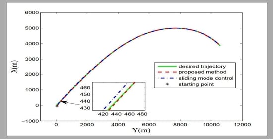
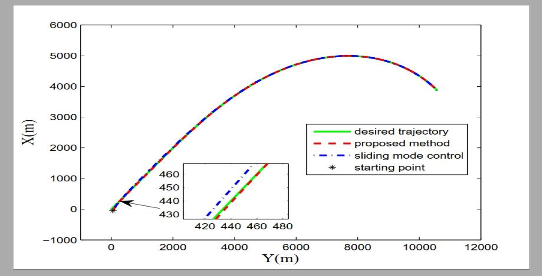
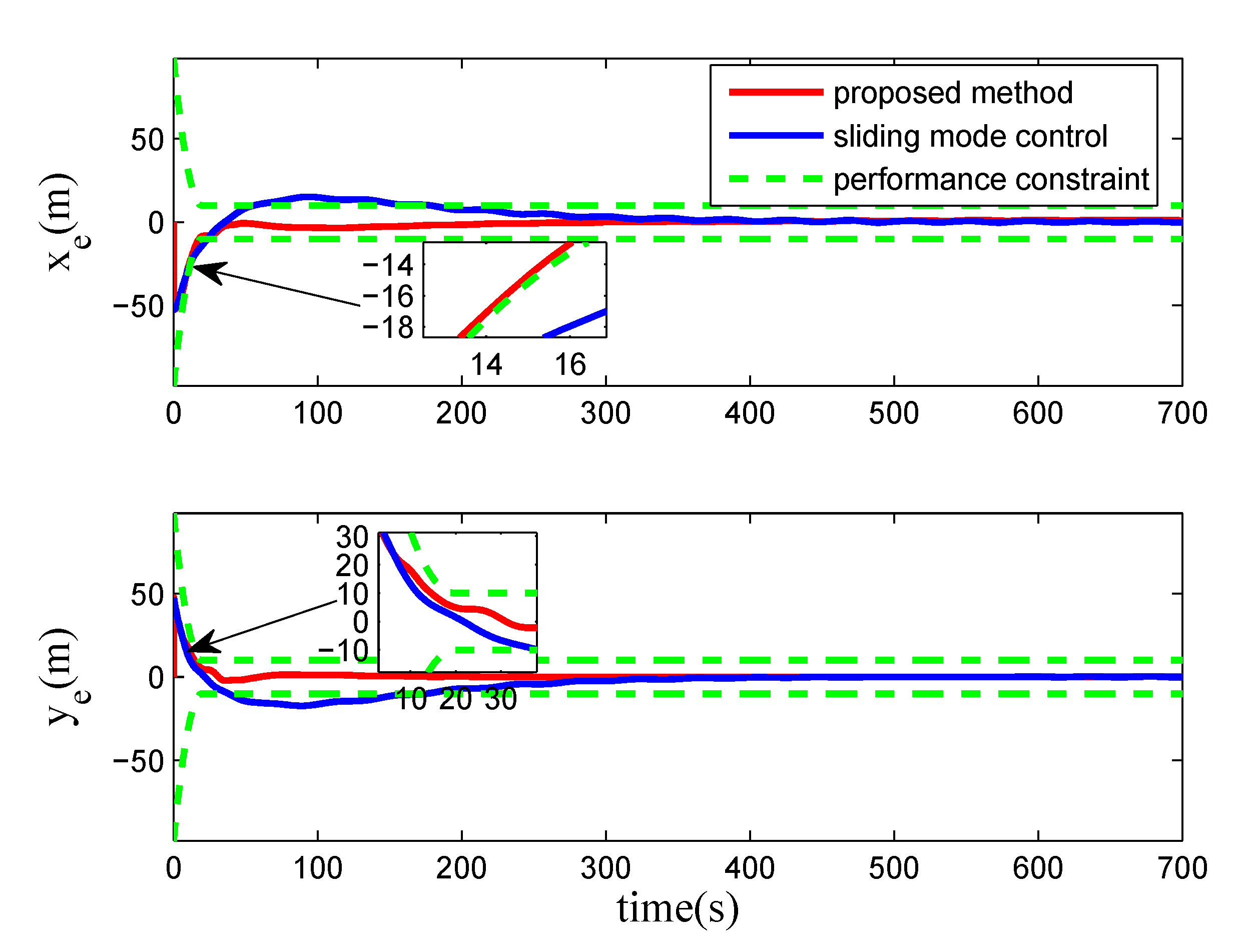
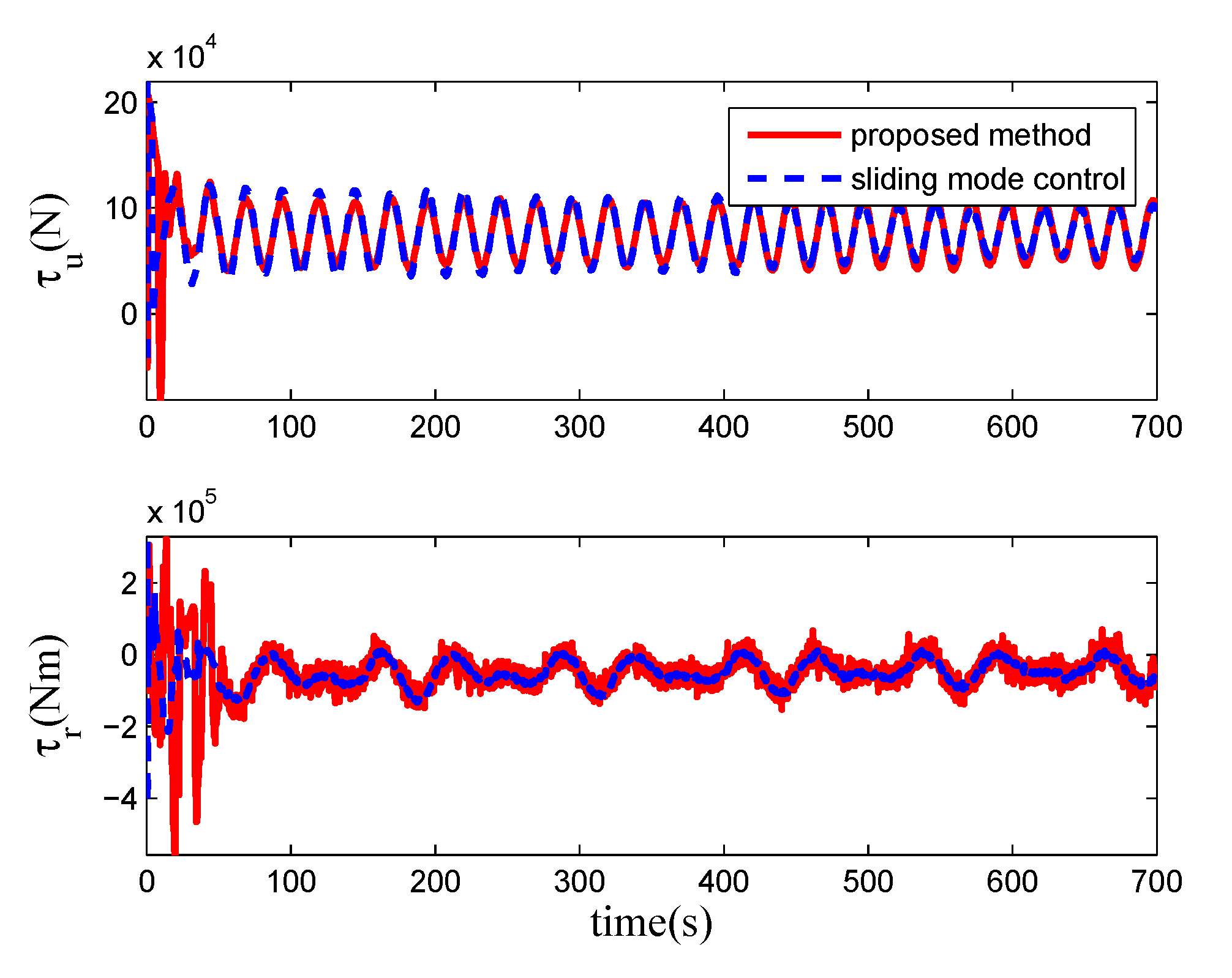
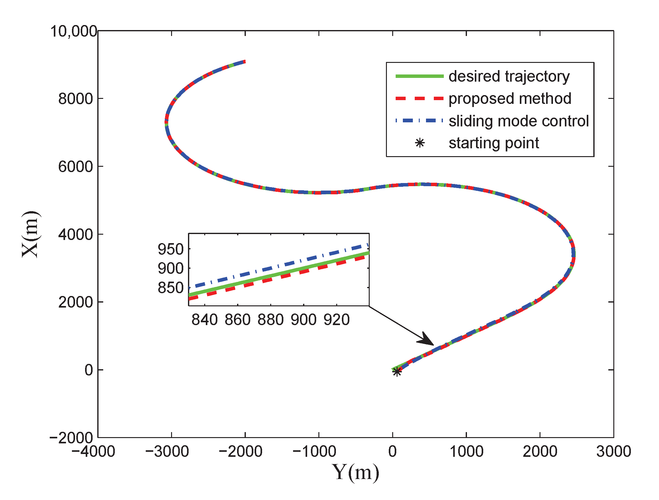
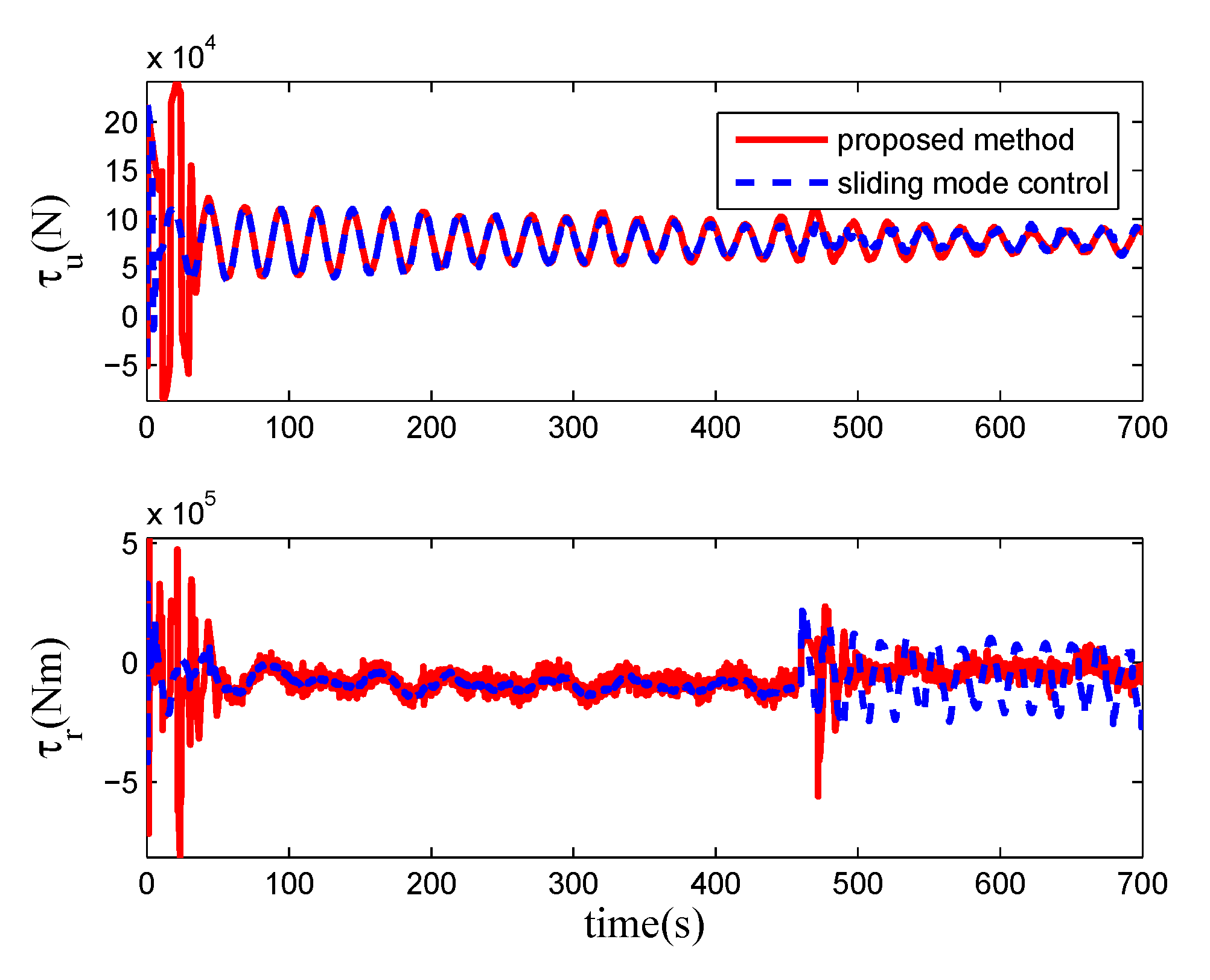
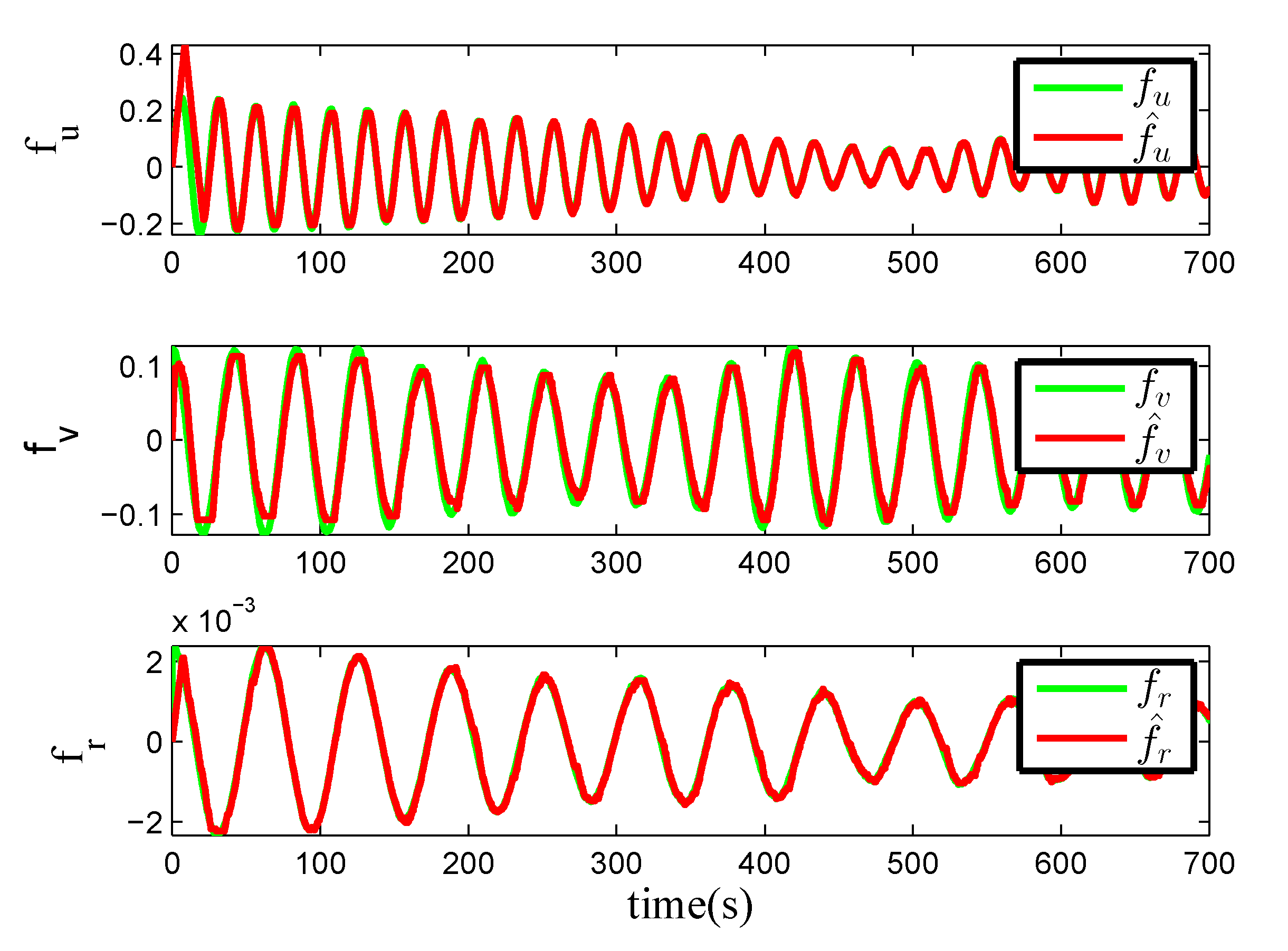
4. Numerical Simulations

The comparison with the finite-time terminal sliding mode control method in [21] is implemented to demonstrate the advantages and effectiveness of the proposed method. In simulations, the major parameters of the hovercraft can be found in [29].
The initial values of the hovercraft under the condition of Assumption 1 are selected as ψ ( 0 ) = 30 , u ( 0 ) = 30 , v ( 0 ) = 0 and r ( 0 ) = 0 . The control parameters are designed as k x = 0.02 , k y = 0.068 , k u = 1.999 , k v = 2.5 and k r = 0.99 . The parameters of the virtual vessel are chosen as x d ( 0 ) = 0 , y d ( 0 ) = 0 , ψ d ( 0 ) = 45 , u d s e t ( t ) = 35 and v d s e t ( t ) = 0 . The hovercraft’s initial position x ( 0 ) , y ( 0 ) and the parameter r d s e t ( t ) of the virtual vessel are given in two cases to show the advantages of the proposed method.
Case 1: The hovercraft’s initial position is selected as x ( 0 ) = 50 , y ( 0 ) = 50 and the parameter r d s e t ( t ) of the desired trajectory is given by:
r d s e t t = 0 t < 100 s a t k r s e t t 100 , 0.5 , 0.5 t 100
Case 2: The hovercraft’s initial position is selected as x ( 0 ) = 60 , y ( 0 ) = 60 and the parameter r d s e t ( t ) of the desired trajectory is given by:
r d s e t t = 0 t < 100 s a t k r s e t t 100 , 0.5 , 0.5 100 t < 460 s a t k r s e t t 100 , 0.5 , 0.5 t 460
where
s a t ( x , x _ m a x , x _ m i n ) = x _ m a x , x > x _ m a x x , x _ m i n x x _ m a x x _ m i n , x < x _ m i n
The parameters of the performance constraint function are designed as k ¯ x b = k ¯ y b = 100 , k x b = k y b = 10 , k ¯ u b = 20 , k ¯ v b = 5 , k ¯ r b = 5 , k u b = 0.6 , k v b = 0.6 , k r b = 0.6 , T x a = T y a = 20 and T u a = T v a = T r a = 60 . Since ARBFNN is used to approximate the model uncertainties f u , f v , and f r , the hidden node numbers for W ^ u T H u Z u , W ^ v T H v Z v and W ^ r T H r Z r are set to n = 13 , with centers of the radial basis functions ϕ l 1 l 1 = 1 , · · · , n , ϕ l 2 l 2 = 1 , · · · , n and ϕ l 3 l 3 = 1 , · · · , n evenly spaced in 1.5 , 1.5 , 1 , 1 and 2 , 2 , respectively. The widths of the radial basis functions are chosen as ε l 1 = 30 , ε l 2 = 20 and ε l 2 = 25 , respectively.
The model uncertainties and external disturbances are described by the following formula:
f u f v f r = 2 sin ( 0.05 t ) m 0 0.2 cos ( 0.03 t ) m 0 cos ( 0.02 t ) J z 0 b 1 b 2 b 3
where b = b 1 b 2 b 3 T R 3 , b ˙ = T 1 b + A w n is the first-order Markov process, w n R 3 is the vector of zero-mean Gaussian white noises, the other parameters of the first-order Markov process are set as:
b ( 0 ) = [ 2 × 10 4 , 2 × 10 4 , 2 × 10 4 ] T T = d i a g ( 10 3 , 10 3 , 10 3 ) A = d i a g ( 1 × 10 4 , 1 × 10 4 , 1 × 10 4 )
The simulation results of the two different methods with and without appointed-time performance constraints under cases 1 and 2 are shown in Figure 2, Figure 3, Figure 4, Figure 5, Figure 6, Figure 7, Figure 8, Figure 9 and Figure 10 and labeled as proposed method and sliding mode control, respectively. It can be known from Figure 2 and Figure 6 that the hovercraft can track the desired trajectory in ideal accuracy under the two different control methods. The desired trajectory is composed of a straight line and a quasi-circle which can represent somewhat realistic performance in the problem of path following or trajectory tracking. It is obvious from Figure 3 and Figure 7 that the proposed method guarantees the pre-specified transient and steady performance boundaries k i a ( t ) , i = x , y of the position tracking errors, in which the appointed-time performance constraints are never violated. The speed and turn rate tracking curves are depicted in Figure 4 and Figure 8, from whose embodied subplot the speed and turn rate tracking errors can always remain within the pre-specified transient and steady performance boundaries k i a ( t ) , i = u , v , r . From further observation in Figure 3, Figure 4, Figure 7, and Figure 8, the performance constraints on the position and sway speed tracking errors for the finite-time terminal sliding mode control method, however, have clearly been violated.
In addition, compared with the finite-time sliding mode control method in [21], the proposed method can guarantee that the position and speed tracking errors converge to a small range around zero within the user-appointed time T i a ( t ) , i = x , y , u , v , r . Thus, the proposed method accelerates clearly convergence time of the control system. The control inputs under these two methods are shown in Figure 5 and Figure 9. It can be observed that the amplitude of the yaw control input τ r under the proposed control method varies rapidly in the initial period in order to track the desired trajectory quickly. The model uncertainties and corresponding estimation values are shown in Figure 10. Accordingly, by analyzing the simulation results under cases 1 and 2, the proposed control method can provide better transient and steady performances and faster convergence speed than the finite-time terminal sliding mode control method in [21].

5. Conclusions

In this paper, we have proposed the control designs for underactuated hovercraft with multiple performance constraints and model uncertainties. A new time-varying appointed-time integral barrier Lyapunov function technique is developed, which is capable of fulfilling position and speed tracking in a user-appointed time while ensuring the evolution of the tracking errors of the position and speed along with the predefined performance constraint bounds. Moreover, compared with existing works, the proposed control method can not only deal with the time-varying constraint on the errors but also ensure that all the tracking errors converge to a small range around zero within user-designing time. Simulation results were carried out to indicate the efficiency and advantages of the proposed method. In future work, the input saturation will be taken into account in the proposed integral barrier Lyapunov function.

Author Contributions

Software and resources, M.F.; conceptualization, methodology and writing—original draft preparation, T.Z.; validation and investigation, F.D.; writing—review and editing, D.W. All authors have read and agreed to the published version of the manuscript.

Funding

The work has been supported by the project “Research on Maneuverability of High Speed Hovercraft” (Project No. 2007DFR80320) and the National Natural Science Foundation of China (Grant No. 51309062).

Conflicts of Interest

The authors declare no conflict of interest.

References

  1. Yun, L.; Bliault, A. Theory and Design of Air Cushion Craft; Elsevier: Amsterdam, The Netherlands, 2000; pp. 458–486. [Google Scholar]
  2. Sun, Z.; Zhang, G.; Yang, J.; Zhang, W. Research on the sliding mode control for underactuated surface vessels via parameter estimation. Nonlinear Dyn. 2018, 91, 1163–1175. [Google Scholar] [CrossRef]
  3. Ashrafiuon, H.; Muske, K.R.; McNinch, L.C.; Soltan, R.A. Sliding-mode tracking control of surface vessels. IEEE Trans. Ind. Electron. 2008, 55, 4004–4012. [Google Scholar] [CrossRef]
  4. Li, T.; Zhao, R.; Chen, C.L.P.; Fang, L.; Liu, C. Finite-time formation control of under-actuated ships using nonlinear sliding mode control. IEEE Trans. Cybern. 2018, 48, 3243–3253. [Google Scholar] [CrossRef] [PubMed]
  5. Zhang, G.; Zhang, X.; Zheng, Y. Adaptive neural path-following control for underactuated ships in fields of marine practice. Ocean Eng. 2015, 104, 558–567. [Google Scholar] [CrossRef]
  6. Zhang, G.; Zhang, X. Practical robust neural path following control for underactuated marine vessels with actuators uncertainties. Asian J. Control. 2017, 19, 173–187. [Google Scholar] [CrossRef]
  7. Ghommam, J.; Chemori, A. Adaptive RBFNN finite-time control of normal forms for underactuated mechanical systems. Nonlinear Dyn. 2017, 90, 301–315. [Google Scholar] [CrossRef]
  8. Lin, X.; Nie, J.; Jiao, Y.; Liang, K.; Li, H. Adaptive fuzzy output feedback stabilization control for the underactuated surface vessel. Appl. Ocean Res. 2018, 74, 40–48. [Google Scholar] [CrossRef]
  9. Qiu, D.; Wang, Q.; Yang, J.; She, J. Adaptive fuzzy control for path tracking of underactuated ships based on dynamic equilibrium state theory. Int. J. Comput. Intell. Syst. 2011, 4, 1148–1157. [Google Scholar] [CrossRef]
  10. Do, K.D. Global robust adaptive path-tracking control of underactuated ships under stochastic disturbances. Ocean Eng. 2016, 111, 267–278. [Google Scholar] [CrossRef]
  11. Do, K.D.; Pan, J.; Jiang, Z.P. Robust adaptive control of underactuated ships on a linear course with comfort. Ocean Eng. 2003, 30, 2201–2225. [Google Scholar] [CrossRef]
  12. Bechlioulis, C.P.; Rovithakis, G.A. Prescribed performance adaptive control for multi-input multi-output affine in the control nonlinear systems. IEEE Trans. Automat. Contr. 2010, 55, 1220–1226. [Google Scholar] [CrossRef]
  13. Wang, W.; Wen, C. Adaptive actuator failure compensation control of uncertain nonlinear systems with guaranteed transient performance. Automatica. 2010, 46, 2082–2091. [Google Scholar] [CrossRef]
  14. Wang, C.; Lin, Y. Adaptive dynamic surface control for MIMO nonlinear time-varying systems with prescribed tracking performance. Int. J. Control. 2015, 88, 832–843. [Google Scholar] [CrossRef]
  15. Bu, X.; Wu, X.; Huang, J.; Wei, D. Robust estimation-free prescribed performance back-stepping control of air-breathing hypersonic vehicles without affine models. Int. J. Control. 2016, 89, 2185–2200. [Google Scholar] [CrossRef]
  16. Psomopoulou, E.; Theodorakopoulos, A.; Doulgeri, Z.; Rovithakis, G.A. Prescribed performance tracking of a variable stiffness actuated robot. IEEE Trans. Control Syst. Technol. 2015, 23, 1914–1926. [Google Scholar] [CrossRef]
  17. Zheng, Z.; Feroskhan, M. Path following of a surface vessel with prescribed performance in the presence of input saturation and external disturbances. IEEE/ASME Trans. Mechatron. 2017, 22, 2564–2575. [Google Scholar] [CrossRef]
  18. Park, B.S.; Yoo, S.J. Robust fault-tolerant tracking with predefined performance for underactuated surface vessels. Ocean Eng. 2016, 115, 159–167. [Google Scholar] [CrossRef]
  19. Chen, L.; Cui, R.; Yang, C.; Yan, W. Adaptive neural network control of underactuated surface vessels with guaranteed transient performance: Theory and experimental results. IEEE Trans. Ind. Electron. 2020, 67, 4024–4035. [Google Scholar] [CrossRef] [Green Version]
  20. Bechlioulis, C.P.; Karras, G.C.; Heshmati-Alamdari, S.; Kyriakopoulos, K.J. Trajectory tracking with prescribed performance for underactuated underwater vehicles under model uncertainties and external disturbances. IEEE Trans. Control Syst. Technol. 2017, 25, 429–440. [Google Scholar] [CrossRef]
  21. Fu, M.; Gao, S.; Wang, C.; Li, M. Human-centered automatic tracking system for underactuated hovercraft based on adaptive chattering-free full-order terminal sliding mode control. IEEE Access. 2018, 6, 37883–37892. [Google Scholar] [CrossRef]
  22. Jin, X. Adaptive fixed-time control for MIMO nonlinear systems with asymmetric output constraints ising iniversal barrier functions. IEEE Trans. Automat. Contr. 2019, 64, 3046–3053. [Google Scholar] [CrossRef]
  23. Tee, K.P.; Ge, S.S. Control of state-constrained nonlinear systems using Integral Barrier Lyapunov Functionals. In Proceedings of the 2012 IEEE 51st IEEE Conference on Decision and Control (CDC), Maui, HI, USA, 10–13 December 2012; pp. 3239–3244. [Google Scholar]
  24. Liu, N.; Shao, X.; Yang, W. Integral barrier lyapunov function based saturated dynamic surface control for vision-based quadrotors via back-stepping. IEEE Access. 2018, 6, 63292–63304. [Google Scholar] [CrossRef]
  25. Xia, J.; Zhang, Y.; Yang, C.; Wang, M.; Annamalai, A. An improved adaptive online neural control for robot manipulator systems using integral Barrier Lyapunov functions. Int. J. Syst. Sci. 2019, 50, 638–651. [Google Scholar] [CrossRef] [Green Version]
  26. Kong, L.; He, W.; Yang, C.; Li, Z.; Sun, C. Adaptive fuzzy Control for coordinated multiple robots with constraint using impedance learning. IEEE Trans. Cybern. 2019, 49, 3052–3063. [Google Scholar] [CrossRef] [Green Version]
  27. Zhang, J. Integral barrier Lyapunov functions-based neural control for strict-feedback nonlinear systems with multi-constraint. Int. J. Control. Autom. Syst. 2018, 16, 2002–2010. [Google Scholar] [CrossRef]
  28. Liu, M.; Shao, X.; Ma, G. Appointed-time fault-tolerant attitude tracking control of spacecraft with double-level guaranteed performance bounds. Aerosp. Sci. Technol. 2019, 92, 337–346. [Google Scholar] [CrossRef]
  29. Fu, M.; Gao, S.; Wang, C.; Li, M. Design of driver assistance system for air cushion vehicle with uncertainty based on model knowledge neural network. Ocean Eng. 2019, 172, 296–307. [Google Scholar] [CrossRef]
  30. Chen, M.; Ge, S.S. Direct adaptive neural control for a class of uncertain nonaffine nonlinear systems based on disturbance observer. IEEE Trans. Cybern. 2013, 43, 1213–1225. [Google Scholar] [CrossRef]
  31. Tee, K.P.; Ge, S.S. Control of nonlinear systems with partial state constraints using a barrier Lyapunov function. Int. J. Control. 2011, 84, 2008–2023. [Google Scholar] [CrossRef]
  32. Zheng, Z.; Sun, L.; Xie, L. Error-constrained LOS path following of a surface vessel with actuator saturation and faults. IEEE Trans. Syst. Man, Cybern. Syst. 2018, 48, 1794–1805. [Google Scholar] [CrossRef]
  33. Fu, M.; Wang, T.; Wang, C. Barrier lyapunov function-based adaptive control of an uncertain hovercraft with position and velocity constraints. Math. Probl. Eng. 2019, 2019, 1–16. [Google Scholar] [CrossRef]
Figure 1. Photo of the hovercraft.
Applsci 10 07381 g001
Figure 2. Trajectory of the hovercraft under case 1.
Applsci 10 07381 g002
Figure 3. Position tracking errors of two methods under case 1.
Applsci 10 07381 g003
Figure 4. Speed and turn rate tracking errors of two methods under case 1.
Applsci 10 07381 g004
Figure 5. Control inputs of two methods under case 1.
Applsci 10 07381 g005
Figure 6. Trajectory of the hovercraft under case 2.
Applsci 10 07381 g006
Figure 7. Position tracking errors of two methods under case 2.
Applsci 10 07381 g007
Figure 8. Speed and turn rate tracking errors of two methods under case 2.
Applsci 10 07381 g008
Figure 9. Control inputs of two methods under case 2.
Applsci 10 07381 g009
Figure 10. Model uncertainties and their estimation values.
Applsci 10 07381 g010
Publisher’s Note: MDPI stays neutral with regard to jurisdictional claims in published maps and institutional affiliations.

