1. Introduction
Grouting, as a method of foundation treatment, is a crucial step in guaranteeing a dam’s safety and reliability [
1]. Generally, the grouting procedures can be arranged in the following five sequences: drilling, washing, water testing, grouting and grouting effects test, which are depicted in
Figure 1. Real-time optimization of grouting process contributes to guaranteeing grouting safety and quality. The grouting pressure and injection rate, which are two key grouting process parameters, are directly related to each other in practical projects, making the relationship between them of considerable importance [
2], and conjoint adjustment of grouting pressure and injection rate reasonably contributes to controlling the grouting quality. Xia [
3] proposed a new indicator, grouting power, which is the product of grouting pressure and injection rate, to link these two parameters. Because the grouting pressure and injection rate are not determined values but fluctuate within upper and lower limits in practical engineering, the grouting power has a certain range; in addition to being influenced by complex geographical conditions and construction conditions, it also exhibits highly nonlinear characteristics. If the grouting power is kept within a certain range, the grouting process is considered to be normal and safe. Nevertheless, the adjustment of the grouting pressure and injection rate is conducted after the appearance of defective grouting conditions in practical engineering, which leads to poor control of the grouting process. Therefore, accurate and real-time prediction of grouting power is of great importance. First, accurate prediction can reflect whether defective grouting conditions will occur in advance. Second, based on the accurate prediction, construction workers can complete the reasonable regulation of the grouting pressure and injection rate to maintain the grouting power within a certain range and realize real-time optimization of the grouting process, guaranteeing grouting safety and quality.
With the rapid development of science and technology, intelligent algorithms have been introduced into the prediction research of grouting projects. Tran and Hoang [
4] developed a groutability prediction model by utilizing support vector regression (SVR) and the differential evolution (DE) algorithm. Hoang et al. [
5] combined SVR with differential flower pollination (DFP) for the prediction of groutability. Deng et al. [
6] combined a support vector machine (SVM) with the hybrid grey wolf optimization algorithm (HGWO) to model groutability of fracture grouting. The back propagation neural network (BPNN) model and artificial neural network (ANN) model were established, respectively, to predict cement take by Yang [
7] and Zhang et al. [
8]. Fan et al. [
9] applied SVR and multivariate regression analysis to predict cement take, and the superiority of SVR model was verified by a higher correlative coefficient. Öge [
10] utilized an adaptive neuro fuzzy inference system (ANFIS) and multiple regression to predict cementitious grout take of mine shaft permeation. Li et al. [
11] applied ANFIS to predict rock quality designation (RQD), permeability (Lugeon value), and fracture filled rate (FFR), then utilized these three predicted indicators to evaluate curtain grouting efficiency. Most of the above research mainly focused on prediction of pre-grouting indicators such as groutability or post-grouting indicators such as cement take and grouting efficiency, and there is little attention paid on grouting power prediction. In addition, grouting power time series are often accompanied by highly nonlinear characteristics, making high-precision prediction a big challenge.
Time series prediction, which has been widely utilized in the field of streamflow [
12], transportation [
13] and dam deformation [
14], among others, is the application of a model to predict future values based on historical data; it is also suitable for grouting power prediction. Currently, three main types of time series prediction models have been proposed: conventional statistical approaches, intelligent methods, and hybrid models [
15]. Conventional statistical approaches, including autoregressive (AR) models [
16] and autoregressive moving average (ARMA) models [
17], are linear regression models, and a linear relationship is supposed between future values and historical values. However, considerable nonlinearity exists in the grouting power time series. Therefore, it is difficult to use conventional statistical approaches to capture the characteristics hidden in the grouting power time series. Artificial intelligence algorithms with good capabilities have emerged recently and are extensively used in time series prediction. ANNs [
18] and SVMs [
19] have flexible nonlinear modelling capability; however, they still have their own drawbacks. For example, NN models have problems of overfitting and are time consuming; meanwhile, sensitivity to parameter selection exists in both NN and SVM models. To overcome the inherent drawbacks of a single model, hybrid models based on the concept of “decomposition–prediction–integration” have been proposed recently and have proven to perform better than any single model alone in various fields, such as in landslide displacement [
20] and hydrology [
21].
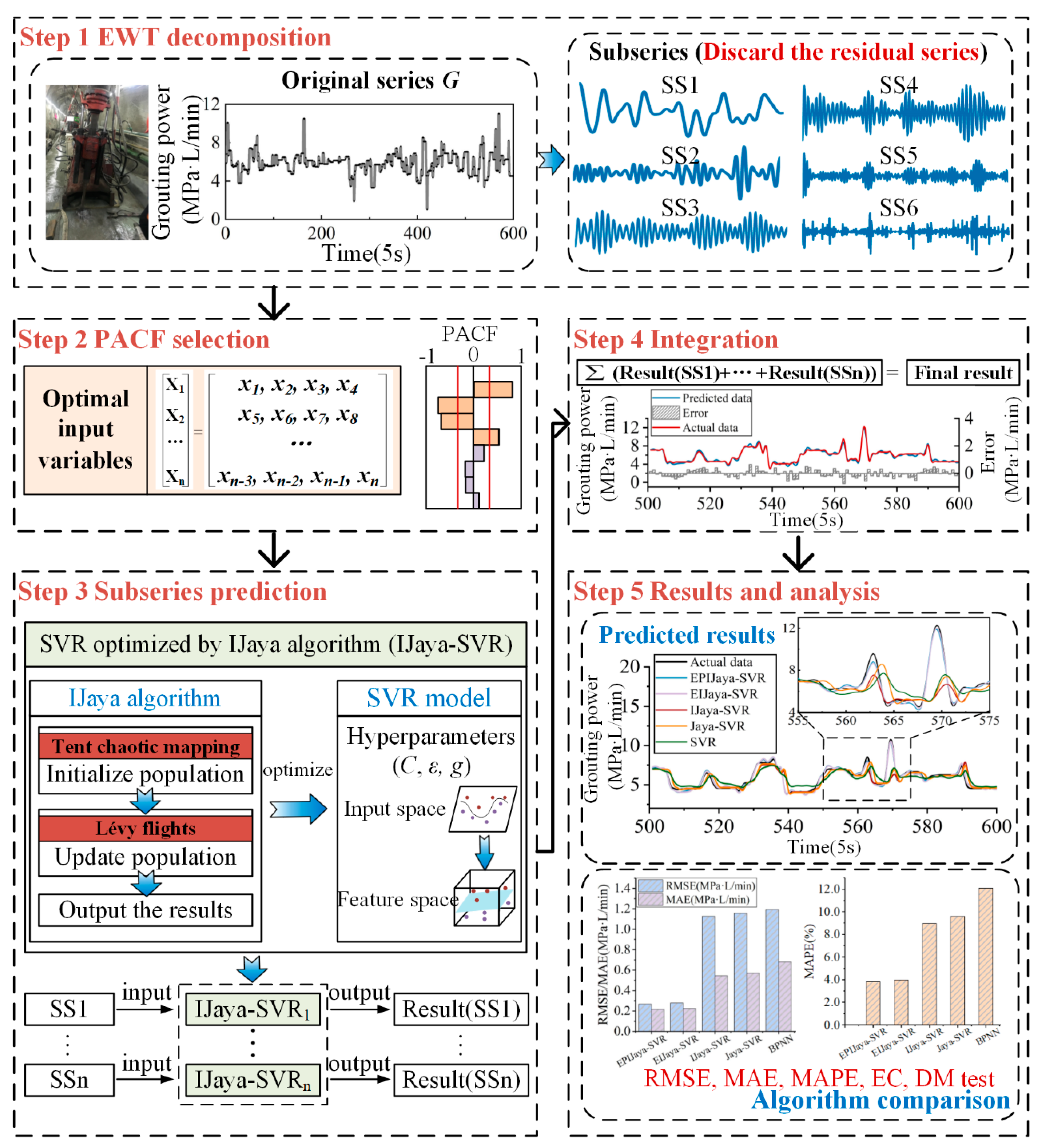
Therefore, a novel hybrid model aiming at overcoming the limitations of single models and obtaining good prediction accuracy is proposed in this study for grouting power time series prediction. This prediction model integrates the merits of the empirical wavelet transform (EWT), the partial autocorrelation function (PACF), SVR, and an improved (IJaya) algorithm and is supposed to achieve better accuracy.
The reminder of this paper is organized as follows: current studies related to the hybrid models based on “decomposition–prediction–integration” are presented in
Section 2. The overall research framework is described in
Section 3.
Section 4 introduces the required individual methodologies, including the EWT, the PACF, SVR, and the IJaya algorithm. In
Section 5 and
Section 6, a case study is performed, and the superiority of the proposed model is verified in comparison with four other competitors.
Section 7 highlights the conclusions.
2. Literature Review
Hybrid models typically combine prediction algorithms with the data decomposition techniques and give full play to the advantages of each component to generate more accurate predictions. As an extension of SVMs, SVR was proposed by Drucker et al. [
22] for regression analysis possessing superior capability in solving multidimensional, nonlinear problems with small samples [
6], and has been proved to be effective in solving various forecasting problems [
23,
24]. Therefore, SVR-based models, which combine the SVR model with data decomposition techniques, are extensively used in time series prediction [
25,
26].
The EWT, which is a novel tool for data decomposition, has been successfully applied in many research areas [
27,
28,
29] and was chosen as a data decomposition technique in this study to preprocess the original grouting power series, by which the original grouting power series is decomposed into a specific number of subseries and one residual series adaptively. When employing SVR models for the decomposed subseries prediction, the prediction performance relies greatly on the input variables and hyperparameters of forecasting components. Hence, identifying optimal input variables and hyperparameters is particularly necessary.
The PACF is used to determine the optimal input variables by calculating the correlation between data [
30,
31,
32]. Meanwhile, identifying the optimal model hyperparameters is an optimization problem. Many studies use optimization algorithms to solve such optimization problems [
33]. One of these methods employs the Jaya algorithm, which is a new population-based optimization method [
34]. The main advantage of this algorithm is the fact that only two common parameters (e.g., the number of generations and the statistical population size) are required and no other specific parameters should be tuned. Unlike the Jaya algorithm, some other meta-heuristic algorithms require algorithm-specific parameters except for the two common parameters. For example, the DE algorithm needs the scaling factor and crossover probability, and the genetic algorithm requires mutation probability, crossover probability, and a selection operator. In addition, the Jaya algorithm only contains one update equation. Because of the above properties, this algorithm is easy to implement. Therefore, the Jaya algorithm has been extensively used in various practical optimization problems such as product design [
35], parameter estimation [
36], and image identification [
37]. Although the Jaya algorithm has been proven to perform well, it still has the problem of premature convergence and becoming trapped in local optima frequently [
38]. To overcome these problems, a new version of the Jaya algorithm is proposed herein. First, tent chaotic mapping has been employed in the Jaya algorithm to initialize the statistical population and preserve statistical population diversity. Moreover, we incorporate Lévy flights into the statistical population updating phase to enhance search capabilities and increase the probability of finding the optimal solution. This improved Jaya (IJaya) algorithm is then used to find the optimal hyperparameters of the SVR model.
Inspired by the concept of hybrid models, a novel hybrid model incorporating the EWT, PACF, SVR and IJaya algorithm is proposed for grouting power prediction based on “decomposition-prediction-integration”. The main aim of decomposition is to simplify the modelling complexity through decomposing the complex grouting power series into relatively simple subseries and one residual series, and denoise the original time series by discarding the residual series. Then the purpose of prediction is to decrease the prediction errors by using appropriate forecasting methods. Finally, the purpose of integration is to yield the final result for the original series by aggregating prediction results of each subseries. The principal contributions of this paper can be summarized as follows:
- (1)
The proposed model not only considers the characteristics of grouting power series but integrates the advantages of four algorithms to remedy the deficiencies of single models, and good prediction accuracy is obtained.
- (2)
An IJaya algorithm is proposed to optimize the hyperparameters of SVR. In the IJaya algorithm, tent chaotic mapping has been employed in the Jaya algorithm to preserve statistical population diversity and prevent the algorithm from sticking on local optima. Also, Lévy flights is introduced to the statistical population updating phase of the basic Jaya algorithm to enhance search capabilities and increase the probability of finding the optimal solution.
- (3)
The EWT is adopted as a data preprocessor to decompose the grouting power series into specific subseries and one residual series to extract meaningful information from the grouting power series. The residual is regarded as an uncorrelated white noise series and discarded to denoise the original grouting power series. The rest subseries are smoother and more predictable, contributing to obtain more precise prediction results.
- (4)
The PACF is applied to calculate the partial correlation between the data in each subseries and identify the optimal input variables for predictors.
4. Methodology
In this study, a novel hybrid model for grouting power forecasting with good prediction accuracy is presented. The main methodologies employed in the proposed hybrid model, consisting of the EWT, PACF, SVR, and IJaya algorithm, are introduced in the following.
4.1. EWT
The EWT, which was proposed by Gilles [
40], is a novel signal processing tool for identifying and extracting different intrinsic modes of time series. It can cope with the shortcomings of some conventional data decomposition techniques: for example, the wavelet transform (WT) [
41] lacks self-adaptive data processing capabilities and has difficulties in selecting a mother wavelet, while empirical mode decomposition (EMD) [
42] and ensemble empirical mode decomposition (EEMD) [
43] face the problem of insufficient mathematical definition.
The EWT relies on powerful peak detection preprocessing to detect the local maximum value of the grouting power time series first, then performs spectrum segmentation, and, finally, generates a series of corresponding wavelet filters. By employing the EWT to decompose the grouting power into a limited number of subseries, good prediction accuracy can be obtained because the temporal variation characteristics in the subseries can be better captured by the prediction model.
First, divide the Fourier support (0, π) into
N continuous segments, denoted as
, where
are the limits of these segments (
). Implement the EWT in the same way used as in the classic WT. The detail coefficient
and approximation coefficient
can then be calculated as follows:
where
is the Fourier transform form of the empirical wavelet function
, and
is the Fourier transform form of the empirical scale function
.
The original signal
is decomposed into specific empirical modes as follows:
4.2. PACF
The grouting power time series is decomposed by the EWT into serval subseries, and the correlation between the data in each subseries is different. Therefore, in the design of the prediction model corresponding to different subseries, the correlation between the data in each subseries needs to be analyzed, and the optimal input variables of each subseries can be determined by analyzing the correlation. Suppose that
is the value needed to be predicted, and only
can be selected as the input variable if all the PACF values are within the 95% confidence interval
. Meanwhile,
is taken as one of the input variables if the partial autocorrelation at lag
p exceeds the 95% confidence interval. For details of the PACF process, see [
44].
The PACF value at lag
p, denoted by
, can be calculated as follows:
where
j = 1, 2, …,
p; p = 1, 2, …,
M, where
M is the maximum lag; and
is the autocorrelation function (ACF) at lag
p.
4.3. SVR Optimized by the IJaya Algorithm
SVR is an effective tool for nonlinear regression and is also suitable for grouting power forecasting. The detailed theory of SVR is presented elsewhere [
45,
46]. The radial basis function kernel, which is the most applicable kernel function [
47], was adopted in this study. Through it, the original data space is mapped into an infinite-dimensional space theoretically. There are three user-determined parameters: the penalty parameter
C, the insensitive loss function
ε, and the kernel function parameter
g; these are critical to the performance of SVR and can be determined by optimization algorithm.
The new Jaya algorithm proposed to solve unconstrained and constrained optimization problems is a simple yet powerful optimization algorithm. Let
O(X) be an objective function that needs to be optimized. Assume that the number of design variables, the statistical population size, and the maximum number of iterations are
Nvar,
Npop, and
Nmax, respectively, and that
i,
j, and
k are their indices, where
,
, and
. If
Xi,j,k stands for the value of the
ith design variable for the
jth candidate during the
kth iteration, then this value can be updated using:
where
presents the upgraded value of
;
and
denote the best solution and the worst solution of the
ith variable during the
kth iteration, respectively;
r1 and
r2 stand for two random numbers with a range of (0,1). Item
indicates the tendency of the solution toward the best solution and item
indicates the tendency to keep away from the worst solution;
is accepted if an improved objective functional value corresponding it is achieved.
The following modifications are integrated into the Jaya algorithm to produce an IJaya algorithm and solve the problems of premature convergence and being trapped in local optima:
The proposed IJaya algorithm applies tent chaotic mapping to initialize the statistical population. The initial statistical population is usually generated randomly, which makes it difficult to ensure its diversity. Chaotic maps exhibit ergodicity, certainty, and the stochastic property, which can effectively preserve statistical population diversity and prevent the algorithm from being trapped in a local optimum [
48]. In this study, tent chaotic mapping is selected to generate the initial statistical population, the steps of which are as follows:
Generate the chaotic variable of
.
where
k is the serial number of the
k-th statistical population and
and
stand for two extreme values of the
i-th variable, which are the minimum and the maximum, respectively.
Apply tent chaotic mapping to generate the chaotic sequence:
Map the chaotic sequence to the search space:
We incorporate Lévy flights into the statistical population updating phase of the basic Jaya algorithm to enhance search capabilities. By employing Lévy flights to update the statistical population, variables can effectively approach their best value through taking short-distance jumps together with occasional long-distance jumps [
49]. By substituting the
updated by Lévy flights, which is represented as
into formula (6), the algorithm’s search ability is enhanced and the probability of finding the optimal solution is improved. For details of Lévy flights, see [
50].
where
represents the random number distributed uniformly,
rand is a random number with a range of (0,1),
stands for entry-wise multiplications.
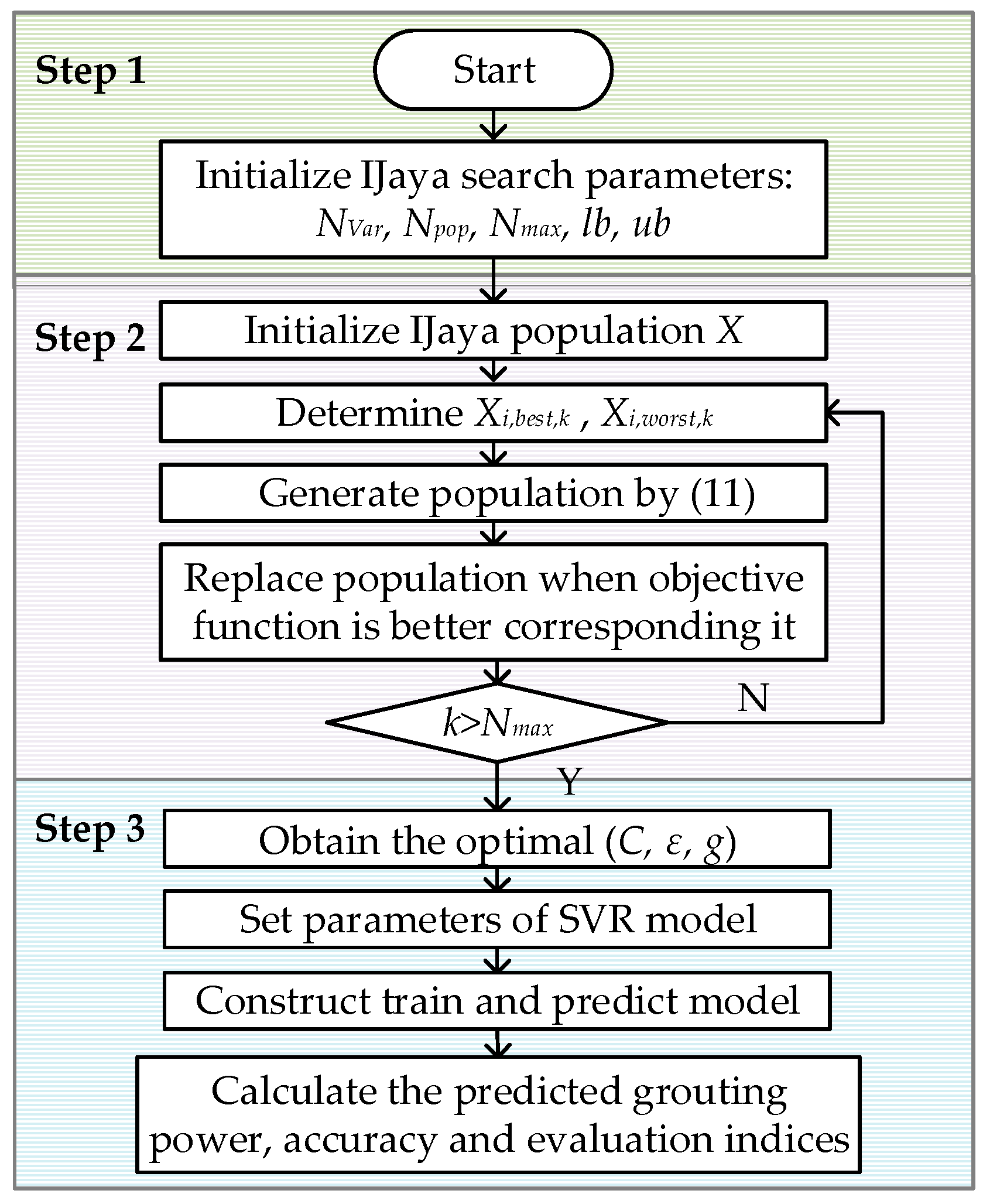
SVR and the IJaya algorithm are combined to construct the prediction model for each subseries. The algorithm consists of the following steps, which are illustrated in
Figure 3 [
6]:
- Step 1.
Parameter initialization
Set the number of design variables, Nvar, the statistical population size Npop, the maximum number of iterations, Nmax, and the lower and upper bounds of the design variables (lb, ub).
- Step 2.
Hyperparameter (C, ε, g) optimization
Initialize the IJaya statistical population, then update the statistical population when the objective function value is better. When iteration k > Nmax, exit the calculation and obtain the optimal (C, ε, g).
- Step 3.
Training and predicting
Based on the hyperparameters obtained from step 2, the training and prediction models are constructed for grouting power prediction. Then the predicted grouting power, accuracy, and evaluation indices are calculated.
5. Case Study
In this section, the proposed hybrid model is applied to predict the grouting power of hydropower project X in China, and its performance is analyzed and discussed. The data collection is described in
Section 5.1.
Section 5.2 provides the performance evaluation criteria. In
Section 5.3, the prediction results of the EPIJaya-SVR model are reported. All experiments are conducted in MATLAB R2017b on Windows 10 with a 2.80 GHz Intel Core i7-1065G7 CPU, 64-bit and 16 GB RAM.
5.1. Data Collection
The proposed hybrid model is applied to a case study to forecast the grouting power of consolidation grouting in hydropower project X, which is located on the Yalong River in Sichuan Province in southwestern China. Hydropower project X is currently under construction; once completed, it will have a hydroelectric generating capacity of 1500 MW and the dam height will reach 155 m. The whole dam can be divided into 17 continuous segments. One grouting hole is selected randomly to serve as the research object. A grouting power dataset of the selected hole is collected with a time interval of 5 s based on a grouting real-time monitoring system. A total of 600 data collected during the grouting process were selected as a sample. Five-hundred data were selected to construct the training set for determining the optimal hyperparameters of the SVR model, while the remaining 100 data were selected as the testing set to evaluate the prediction performance of the obtained model. The statistical information i.e., maximum, minimum, mean, standard deviation and median of this grouting power series are calculated and given in
Table 1.
Figure 4 shows the shapes of the grouting pressure, injection rate, and grouting power.
5.2. Evaluation Criteria
To compare the prediction performance of the proposed hybrid model EPIJaya-SVR with that of four selected competitors (EIJaya-SVR, IJaya-SVR, Jaya-SVR, and SVR), no single evaluation index can reflect the distributional characteristics of the errors. Therefore, four indices—the root mean square error (RMSE), mean absolute percentage error (MAPE), mean absolute error (MAE), and equal coefficient (EC)—are used as forecasting accuracy measures. The model with lower RMSE, MAE, and MAPE and higher EC (closer to 1) can predict grouting power more effectively.
In addition to these evaluation indices, the Diebold–Mariano (DM) test [
51] is also adopted to verify whether the prediction performance of two models is significantly different. The null hypothesis of the DM test assumes that the prediction accuracy of the tested model is not as good as that of the reference model. To be specific, the prediction error
of the tested model is greater than or equal to the prediction error
of the reference model. The DM statistic can be expressed as:
where
is the mean value of the loss function
(
);
(
where
is the variance of
; and
and
denote the predicted values of
calculated by using the tested model
te and reference model
re, respectively.
The DM statistic obeys a standard normal distribution and α is set to be the significance level. Zα/2 is the critical value of the test. If |DM| ≤ |Zα/2|, there is not enough evidence to suggest that the two models exist significant difference, and, if |DM| > |Zα/2|, the null hypothesis can be rejected.
5.3. Simulation
The grouting power time series was submitted into the proposed model to obtain the predicted results in the simulation. The whole flow of the simulation for the grouting power prediction is shown in the following subsections.
5.3.1. Decomposition Process
As shown in
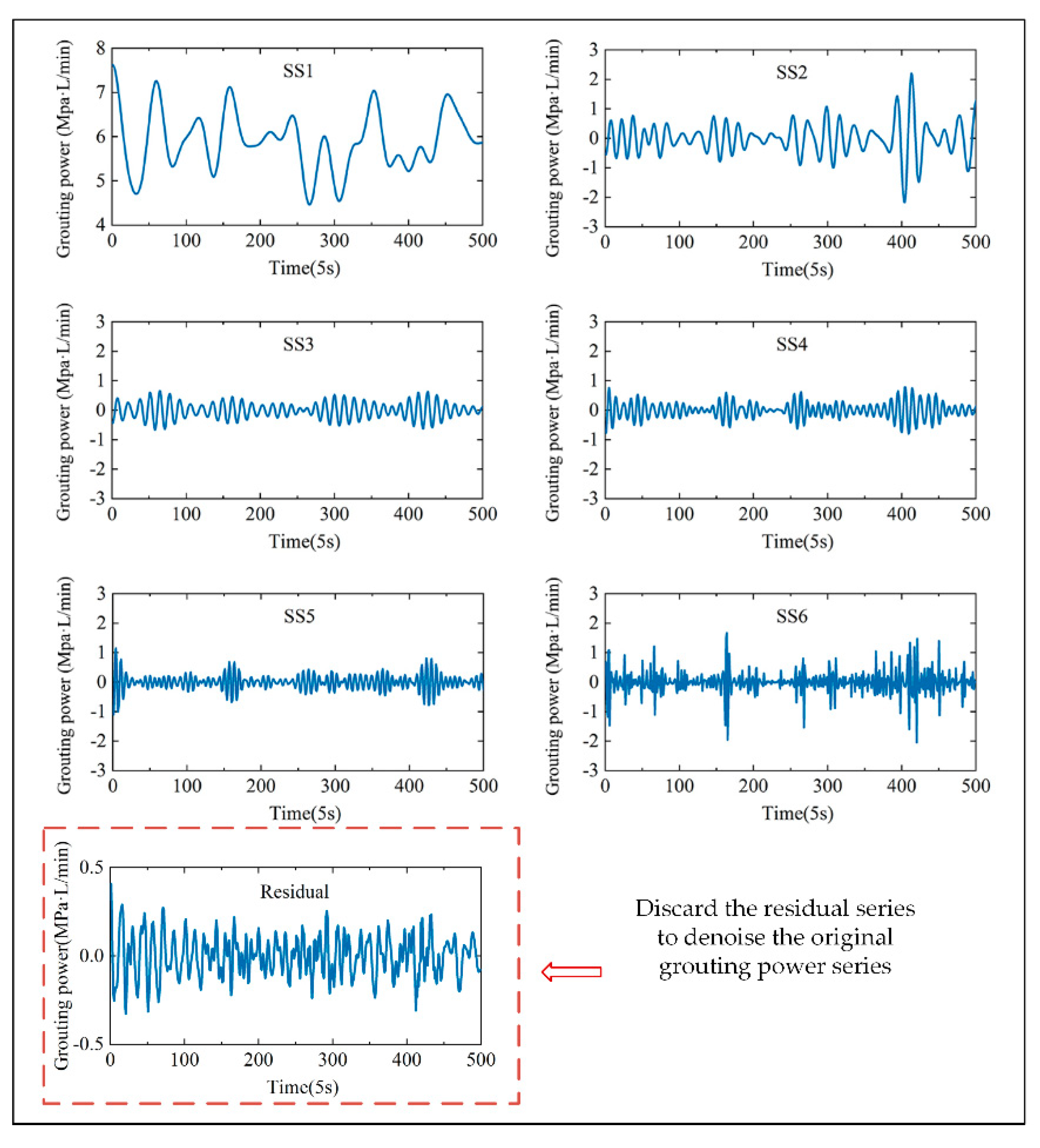
Figure 4, the original grouting power series has large fluctuations, with values falling in the range (1.044, 11.025). Therefore, the EWT was employed to decompose the original grouting power series into six subseries and one residual series to denoise and reduce the modelling complexity of the grouting power series.
Figure 5 illustrates the graphical representation of the decomposed results.
5.3.2. PACF Results
According to the description of the PACF in
Section 4.2, a correlation analysis was conducted for the data elements in each subseries. The length
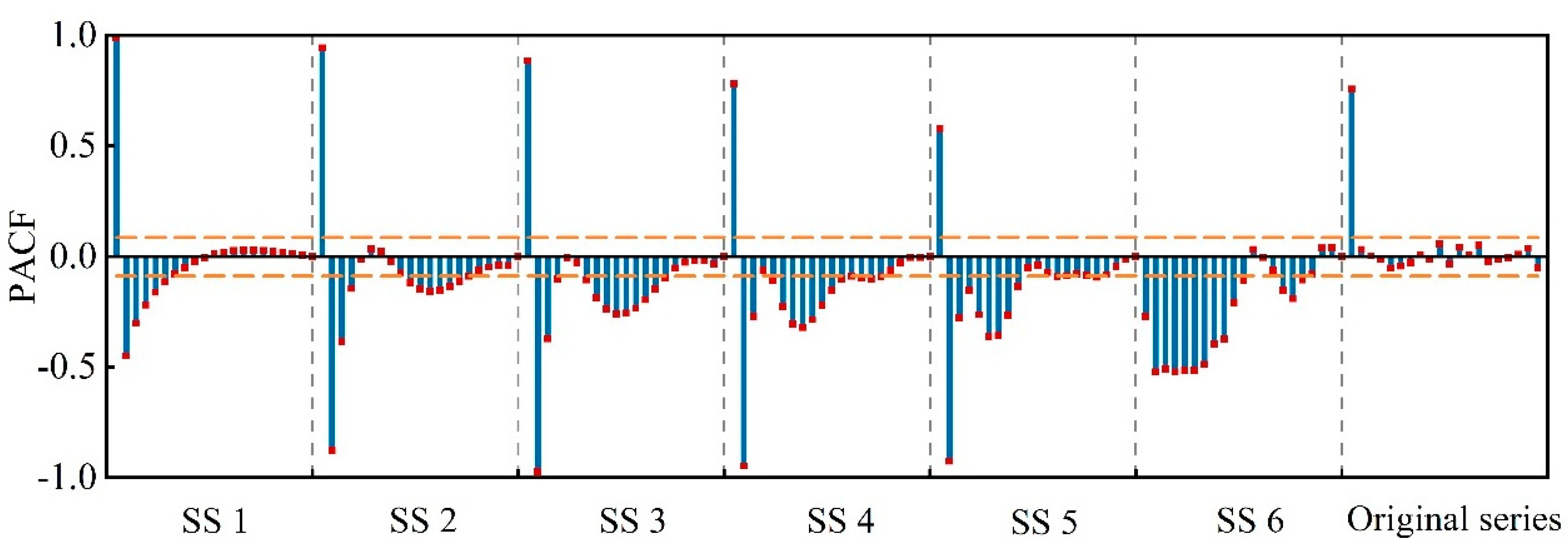
N of the grouting power series was 500, and its 95% confidence interval was (0.0877, +0.0877). The PACF values from lag 1 to lag 20 were calculated and are depicted in
Figure 6.
Figure 6 displays the characteristics of the partial autocorrelation of the original grouting power and the subseries. There is only one variable that can be selected to serve as the input variable for the original grouting power because of the large fluctuation. Nevertheless, more related variables can be selected for each subseries, because the subseries decomposed by the EWT have certain stability and regularity. Consequently, it is easy to establish a prediction model using the subseries than using the original grouting power series.
5.3.3. Prediction and Integration Processes
The SVR model optimized by using the IJaya algorithm was employed as an independent prediction tool to capture the nonlinear patterns of each subseries after the optimal input variables were identified by using the PACF. The predicted value of grouting power was then obtained by summing the predicted results of the subseries. The search ranges of the SVR algorithm were set to
C = (1,1000),
g = (0,10), and
ε = (0,0.2). The statistical population size,
Npop, was set to 30 and the maximum number of iterations,
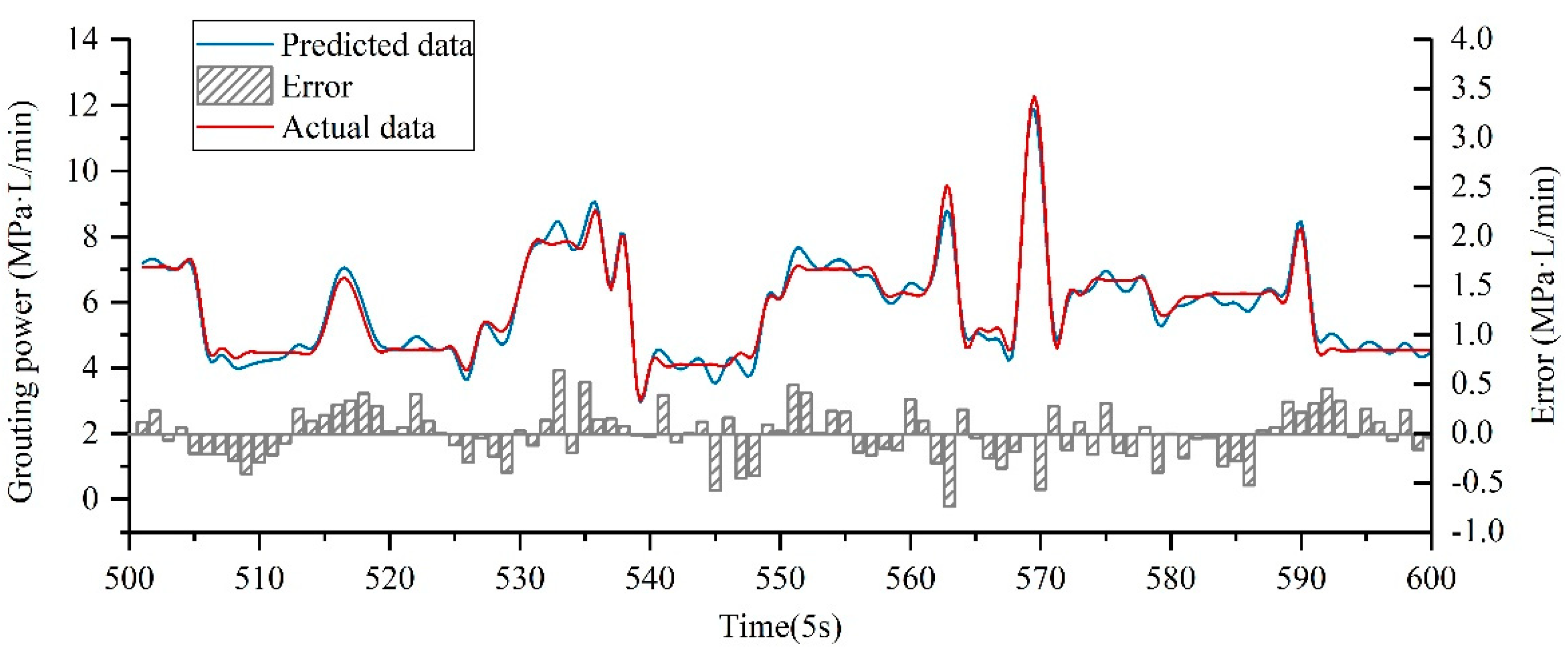
Nmax, was set to 100. The final prediction results are presented in
Figure 7.
Based on accurate, real-time prediction of grouting power during the grouting process, construction workers can regulate the grouting pressure and injection rate reasonably to maintain the grouting power within a certain range, thereby avoiding the occurrence of defective conditions. From the curves of predicted data and actual data in
Figure 7, it can be seen that the prediction error of grouting power based on the EPIJaya-SVR model is small (the average absolute error being 0.2165 MPa·L/min). The predicted and actual data have good consistency, which can meet actual engineering needs, and thus the model proposed here can provide practical assistance for guiding grouting construction.
6. Discussion
In this section, the influence of different statistical population size on IJaya algorithm and prediction performance of different models are discussed to verify the superior prediction ability of the proposed model.
(1) Comparison of different statistical population size
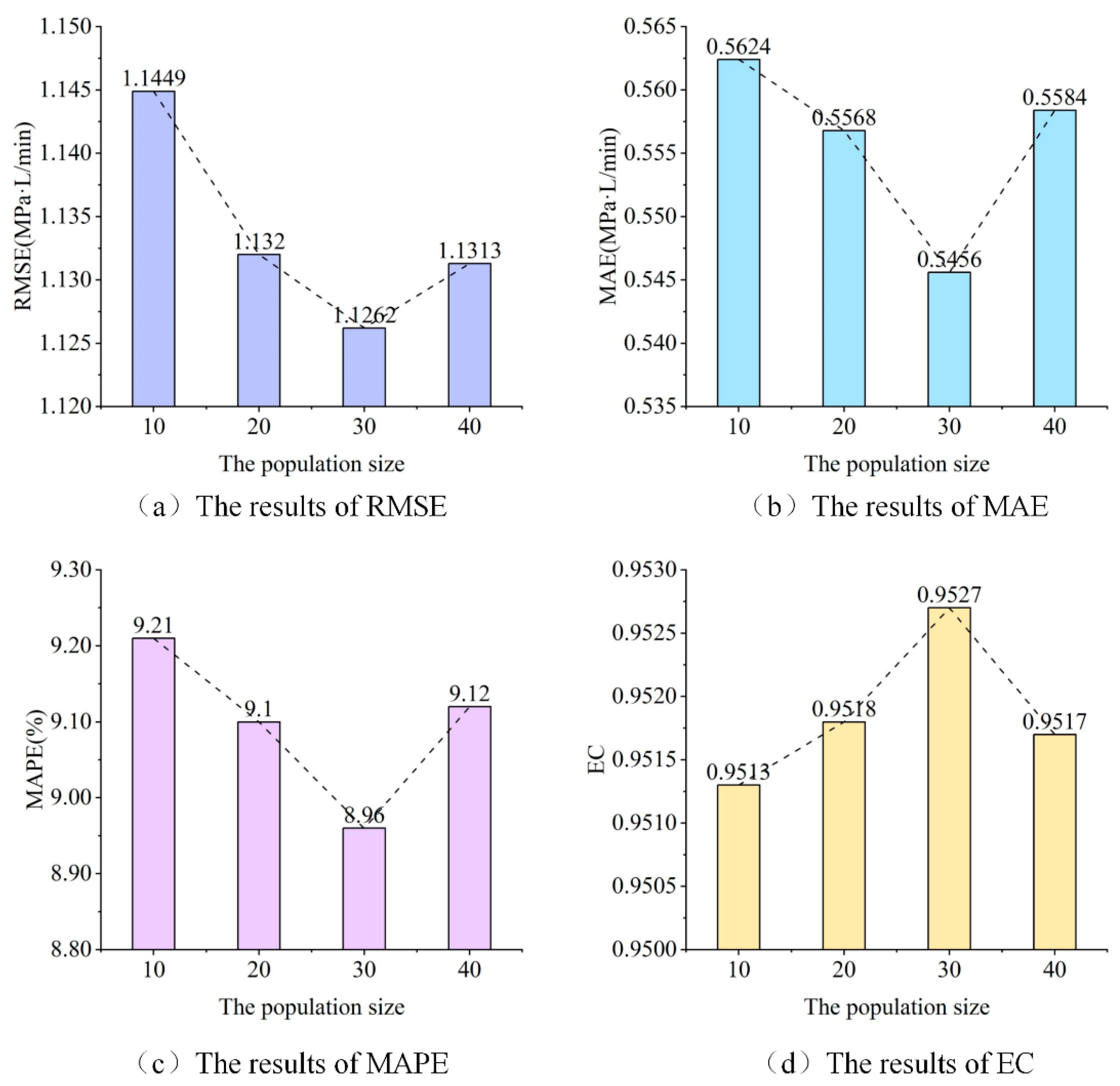
Suitable statistical population size is beneficial to enhance the optimization ability of IJaya algorithm. In order to find the optimal statistical population size of IJaya algorithm in terms of grouting power prediction, different sizes which are 10, 20, 30, 40 are chosen. The comparison results are depicted in
Figure 8.
From
Figure 8, a conclusion can be drawn that the optimization ability of IJaya algorithm is best when the statistical population size is 30. When decreasing the statistical population size of IJaya algorithm from 30, the performance of this algorithm gets worse. What’s more, when increasing the statistical population size beyond 30, the performance also gets worse. Therefore, the statistical population size is chosen as 30 in this paper.
(2) Prediction performance of different models
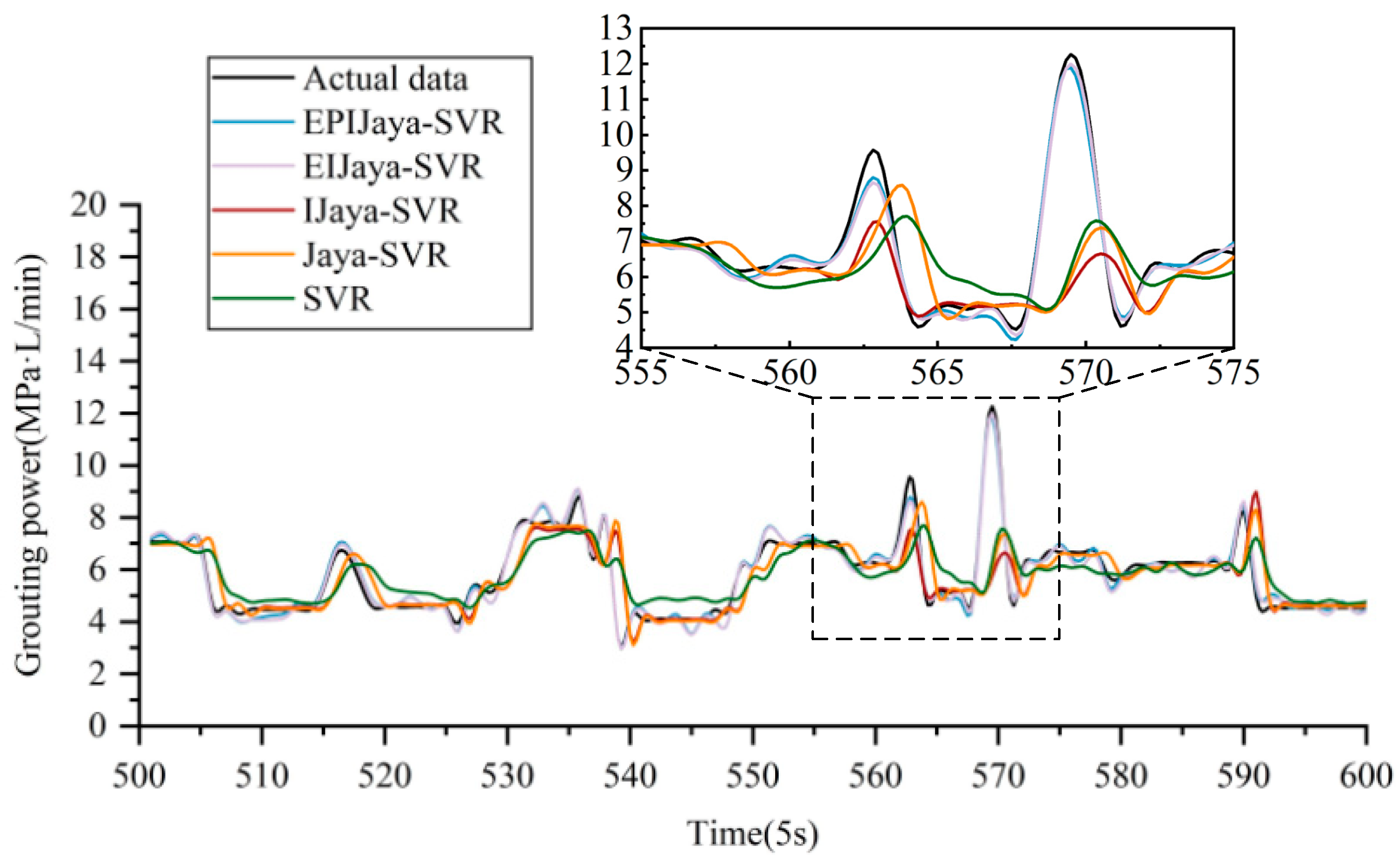
It can be seen from above that the performance of EPIJaya-SVR in grouting power prediction is good, but it still needs to be compared with the other models (EIJaya-SVR, IJaya-SVR, Jaya-SVR, and SVR) considered here. EIJaya-SVR uses the historical values from lag 1 to lag 20 to construct input vectors for each subseries, and the other models all use the PACF to construct the optimal input vectors. The final prediction results of these five prediction models are depicted in
Figure 9, and the results of the four performance indices and the DM test are listed in
Table 2 and illustrated in
Figure 10.
From
Table 2 and
Figure 10, through the comparison of all the models, it is obvious that the EPIJaya-SVR model shows the best performance by obtaining the best RMSE, MAE, MAPE, and EC values of 0.2672 MPa·L/min, 0.2165 MPa·L/min, 3.85%, and 0.9815, respectively. Though the prediction performance of the EIJaya-SVR model with RMSE, MAE, MAPE, and EC values of 0.2788 MPa·L/min, 0.2252 MPa·L/min, 4.00%, and 0.9806, respectively, is little worse than that of the EPIJaya-SVR model, it still performs better than any other single model. This means that the EWT plays a significant role in improving prediction accuracy by denoising and transforming the nonlinear grouting power series into several relatively stable and regular subseries.
In general, the performance of forecasting models is supposed to be enhanced by a carefully selected set of input variables because the nonlinear features of grouting power can be effectively captured. However, the input variables for predictors are determined artificially, which leads to poor prediction accuracy. In this study, the PACF was employed to select variables objectively, thereby effectively avoiding the subjectivity and randomness caused by manual selection. As given in
Table 2 and shown in
Figure 10, the proposed hybrid model betters EIJaya-SVR with reductions of about 4.16%, 3.86%, and 3.75% in the values of RMSE, MAE, and MAPE and a 0.09% rise in the EC value. Hence, utilizing the PACF to select variables reasonably as the input vectors can improve prediction accuracy.
It also can be clearly observed from
Table 2 and
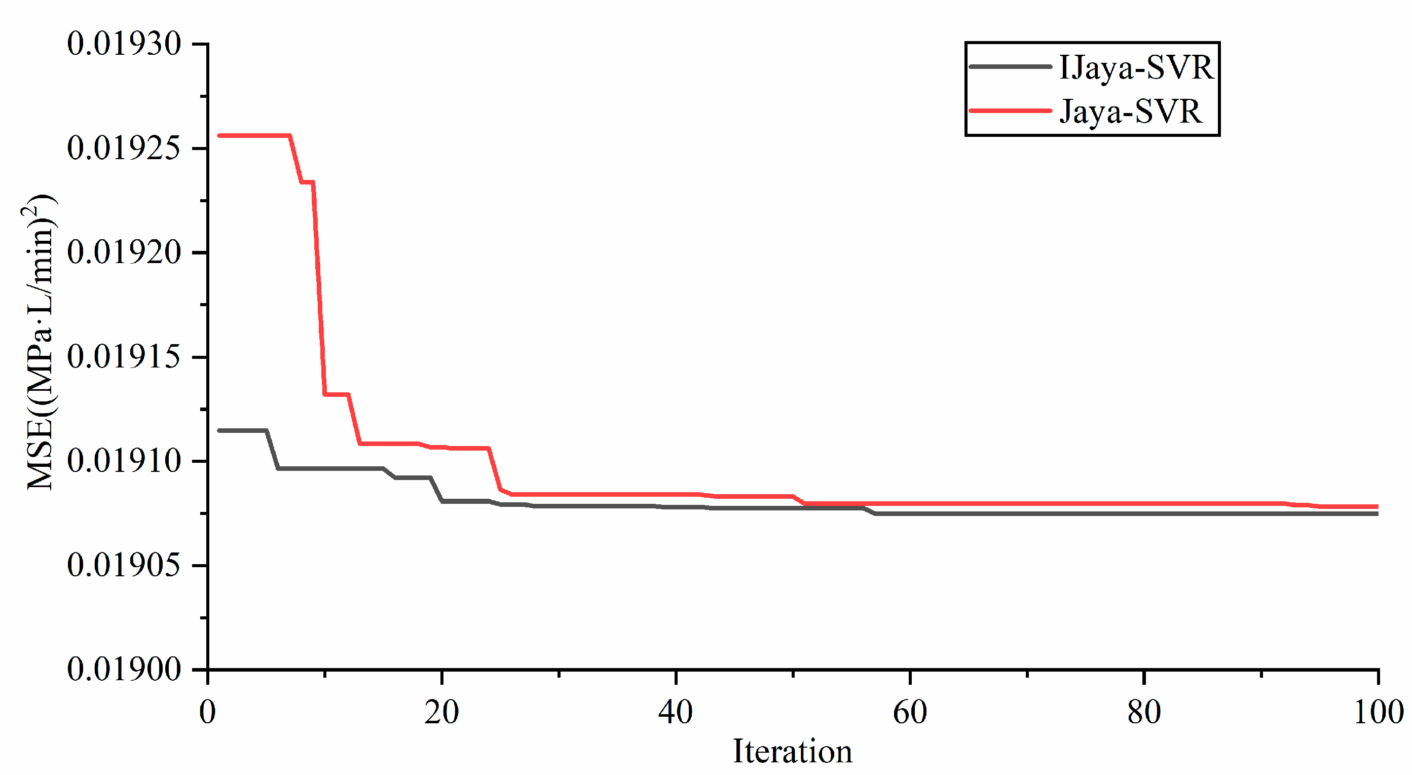
Figure 10 that IJaya-SVR and Jaya-SVR models outperform the SVR model with lower values of RMSE, MAE, MAPE and higher values of EC. This demonstrates the prediction ability of SVR model can be improved by adopting optimization algorithm to optimize hyperparameters. Besides, IJaya-SVR offers significant prediction superiority over Jaya-SVR with lower values of RMSE (1.1262 MPa·L/min), MAE (0.5456 MPa·L/min), and MAPE (8.96%) and a higher EC (0.9527). To some extent, these results come from the IJaya algorithm using tent chaotic mapping to generate the initial statistical population and introducing Lévy flights into the statistical population updating process in the basic Jaya algorithm to obtain the preferable hyperparameters (
C,
ε,
g) of the prediction model; therefore, IJaya-SVR can achieve better precision.
The convergence curve is illustrated in
Figure 11.
The DM test was also adopted to identify the statistical significance of the above models to further evaluate the prediction performance of the tested models. From the results in
Table 2 and
Figure 10, though the superiority of the proposed model over EIJaya-SVR is not obvious, the proposed model is superior to IJaya-SVR, Jaya-SVR, and SVR models at the 1% significance level, with the test results all above the critical value of the 1% significance level (
Z0.01/2 = 2.58). A conclusion obtained from the above analysis is that the hybrid model offers better performance than single models based on statistical thinking.
Actually, because the original grouting power is influenced by complex geological and construction conditions during the grouting process, it is too complex to be predicted accurately by employing a single model. Based on the above analysis, through the organic combination of the EWT, the PACF, SVR, and the IJaya algorithm, the proposed hybrid model has the best performance among all the models considered and can be effectively used for grouting power prediction. Based on the accurate prediction results, construction workers can identify whether the defective grouting conditions will occur in advance. If the predicted grouting power is out of the certain range, regulating the grouting pressure and injection rate to maintain it within the certain range to realize real-time optimization of the grouting process by which grouting safety and quality can be guaranteed.
7. Conclusions
For the sake of controlling the grouting process properly to guarantee grouting safety and quality, accurate and effective methods for grouting power prediction are urgently needed. However, grouting power time series exhibit highly nonlinear characteristics, making it difficult to predict grouting power accurately using a single model. The concept of “decomposition–prediction–integration” is applied to build a hybrid prediction model for grouting power. This model achieves high accuracy by linking the merits of the EWT, the PACF, SVR, and an IJaya algorithm. To be specific, the SVR model is used to predict the grouting power, and the IJaya algorithm, which introduces chaos theory and Lévy flights into the basic Jaya algorithm to improve the algorithm’s accuracy performance, is employed to optimize the hyperparameters of SVR. Moreover, prior to prediction, the EWT as a preprocessor is employed to decompose the original grouting power time series into several subseries and one residual series adaptively, by which meaningful information from the original series is extracted, and the modelling complexity is reduced sharply. The noise in the original grouting power series can be removed by discarding the residual series. Then, the PACF is utilized to determine the optimal input variables for the predictor of each subseries by calculating the correlation between the data to avoid the subjectivity caused by manual selection. Real-word simulations demonstrate that the proposed hybrid model has better prediction performance with higher accuracy compared with four other prediction models in terms of four evaluation indices and the DM test, and it can provide a feasible technical reference for guiding grouting construction.
In future research, the grouting power can be timely predicted by embedding the grouting power prediction model in a real-time grouting monitoring system. This would enable construction workers to regulate the grouting pressure and injection rate before the occurrence of defective grouting conditions, effectively guaranteeing grouting safety and quality.

