Article

Forecasting of Power Demands Using Deep Learning

1
IT Application Systems Engineering, Jeonbuk National University, Jeonju 54896, Korea
2
Advanced Electronics and Information Research Center, Jeonbuk National University, Jeonju 54896, Korea
3
School of International Engineering and Science, Jeonbuk National University, Jeonju 54896, Korea
*
Authors to whom correspondence should be addressed.
These authors contributed equally to this work.
Appl. Sci. 2020, 10(20), 7241; https://doi.org/10.3390/app10207241
Submission received: 19 September 2020 / Revised: 9 October 2020 / Accepted: 13 October 2020 / Published: 16 October 2020

Abstract

:
The forecasting of electricity demands is important for planning for power generator sector improvement and preparing for periodical operations. The prediction of future electricity demand is a challenging task due to the complexity of the available demand patterns. In this paper, we studied the performance of the basic deep learning models for electrical power forecasting such as the facility capacity, supply capacity, and power consumption. We designed different deep learning models such as convolution neural network (CNN), recurrent neural network (RNN), and a hybrid model that combines both CNN and RNN. We applied these models to the data provided by the Korea Power Exchange. This data contains the daily recordings of facility capacity, supply capacity, and power consumption. The experimental results showed that the CNN model outperforms the other two models significantly for the three features forecasting (facility capacity, supply capacity, and power consumption).

1. Introduction

The commercial electric power companies struggle to provide end-users with stable and safe electricity. Therefore, designing efficient forecasting models is a vital step for the planning of the operation of electronic power systems. The demand patterns of electricity could be affected by various factors such as time, economy, social, and environmental factors [1,2].
The power forecasting models can be classified based on their predictive ability into short-term, medium-term, and long-term. Short-term power forecasting models predict up to 1 day/week ahead and used for scheduling the generation and transmission of electricity, medium-term power forecasting models predict for 1 day/week to 1 year ahead and used for fuel preparation, long-term power forecasting models predict more than 1 year and used for developing power supply and delivery system [3,4,5].
Power demands prediction frameworks can be divided into statistical models, grey models, and artificial intelligence models [6]. In statistical models, the correlation between the inputs and the outputs is statistically figured out using empirical models such as log–linear regression models, co-integration analysis and autoregressive integrated moving average (ARIMA), combined bootstrap aggregation (bagging), and exponential smoothing. In the grey models, the researchers integrated a partial theoretical structure with empirical data to build the structure and as result, a limited amount of data are required to infer the behavior of the electrical systems. In artificial intelligence models, they learn to model complex relationships between the outputs and inputs based on the available training data.
Different techniques have been applied in electricity demand forecasting including time series models [7], holt-winters and seasonal regression [8], multiple linear regression [9,10], first-order fuzzy time series [11], autoregressive integrated moving average (ARIMA) [12], seasonal ARIMA (SARIMA) [2], support vector machine (SVM) [13], support vector regression [14], Least square SVM (LSSVM) [1], and artificial neural network (ANN) [10,14,15].
For example, the work conducted by [11] used the monthly demand data from 1970 to 2009 as a training dataset and 2010 data as a testing dataset. The electricity demand in Thailand was predicted by including gross domestic product, maximum ambient temperature, and the population. These features were used as input to a neural network [10]. The authors of [14] used Bayesian regularization in the autoregressive neural network for electricity demand forecasting. Authors in [16] compared different forecasting methods such as neural networks, fuzzy logic, and autoregressive process, and as a result, they found that neural networks and fuzzy logic are more accurate that autoregressive processes. Different techniques were combined by the authors of [17] in which they combined the support vector machine, neural networks, autoregressive integrated moving average, and generalized regression neural network. The authors of [18] proposed a traditional feed-forward neural network with one output node that can predict peak load in one hour or one day in the future. Also, the researchers explored radial basis function networks [19], recurrent neural networks [20], and self-organizing maps [21].
All of these traditional methods have a limited performance as they require hand crafted features. Therefore, with the advancement of deep learning, researchers have utilized different deep learning architectures for several electricity demand forecasting problems [22,23,24,25,26,27]. Different resolutions have been studied from multiple times a day such as monthly [22], weekly [27], daily [24,25,26,27], every two hours [25], hourly [27], half-hourly [23,24,25], minute-by-minute [27]. These models studied different targets such as business consumer [23,25], household consumer [24,27], other than business or household consumer [22], and region/country such as UT Chandigarh, India, in [26].
In this paper, we studied the performance of deep learning models such as convolution neural network (CNN) and recurrent neural network (RNN) for electricity demand forecasting. Unlike previous works [28] that include year and month index to electricity consumption, we use only the daily demand as an input to our predictive models. We designed different deep learning models such as convolution neural network (CNN), recurrent neural network (RNN), and a hybrid model that combines both CNN and RNN. We applied these models to the data provided by the Korea Power Exchange. We built an independent model for each feature namely facility capacity, supply capacity, and power consumption. The experimental results showed that the CNN model outperforms the other two models significantly for the three features forecasting.

2. Materials and Methods

In this section, we introduce the dataset used for this study and the design of the proposed models.

2.1. Materials

In this paper, we used the data from the Korea Power Exchange. It contains recordings from 2003.01.01 to 2020.05.22. The available measurements were taken daily in this dataset—we have 6352 records. The available information is facility capacity, supply capacity, maximum power consumption, supply reserve, and supply reserve ratio. Here, we are interested in predicting the future demands of facility capacity, supply capacity, and maximum power consumption. The statistical overview of these features is given in Table 1. We split that dataset into three parts. The training data contains the records within the first 11 years (from 2003 to 2013), The validation data contains the records within the following three years (from 2014 to 2016). Testing data contains the consumption within the remaining years (from 2017 to 2020). Figure 1 shows the patterns of the available features in the dataset within the study period.

2.2. Data Preprocessing and Preparation

The dataset was normalized to unit norm. To prepare the training, validation, and test sets, we studied different scenarios by varying the history to be used for predicting future demands. We tested different values of the history for predicting different future demands. The history values were set to 7-days,15-days, 30-days, 45-days, and 60-days in the past. On the other hand, we tried to predict future demands after 1-day, 7-days, 15-days, 30-days, 45-days, and 60-days. As a result, we had to study 5 × 6 = 30 possible cases to see the best performing model that we can use for future demands prediction. Figure 2 shows an example of preparing the dataset for 15-days in the past to predict the demands 7-days ahead.

2.3. The Proposed Models

We designed different deep learning models, namely convolution neural network (CNN) [29], recurrent neural network (RNN) [30], and a hybrid model that combines CNN with RNN. We aimed to find the best performing model according to the past and future data of our dataset.
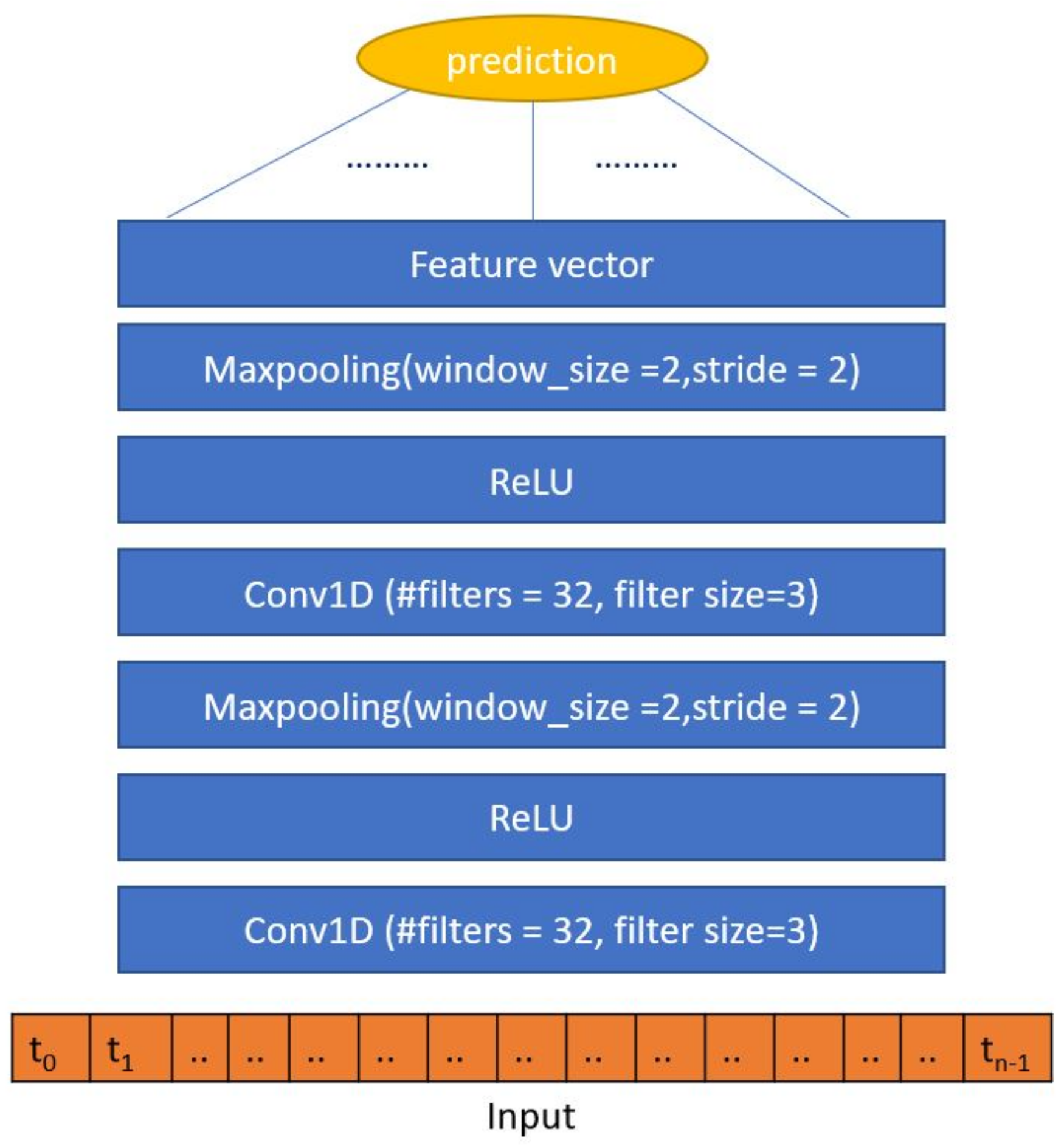
CNN model is a type of deep neural network that is utilized in various domains. It is also considered as a shift-invariant model as they have translation invariance characteristics and shared-weights architecture. CNN models were widely and successfully used in different areas such as image and video classification, medical image analysis, natural language processing, bioinformatics, and time-series. In this work, we designed a simple two-layer CNN model as shown in Figure 3. Each layer consists of a 1-dimensional convolution layer with 32 filters and a filter size of 3, a non-linear activation function which is the rectified linear unit (ReLU), and a max-pooling layer with window size and stride of 2. The learned features from these two layers are then fed into a fully connected layer with a one-node for prediction. The convolution layer is a 1-d convolution expressed in Equation (1) where I is the input, k, and o are the indices of kernels and the output position, respectively, W f is the weight matrix of S × N shape with S filters and N channels.
Conv ( I ) o k = ReLU s = 0 S 1 n = 0 N 1 W s n f I o + s , n
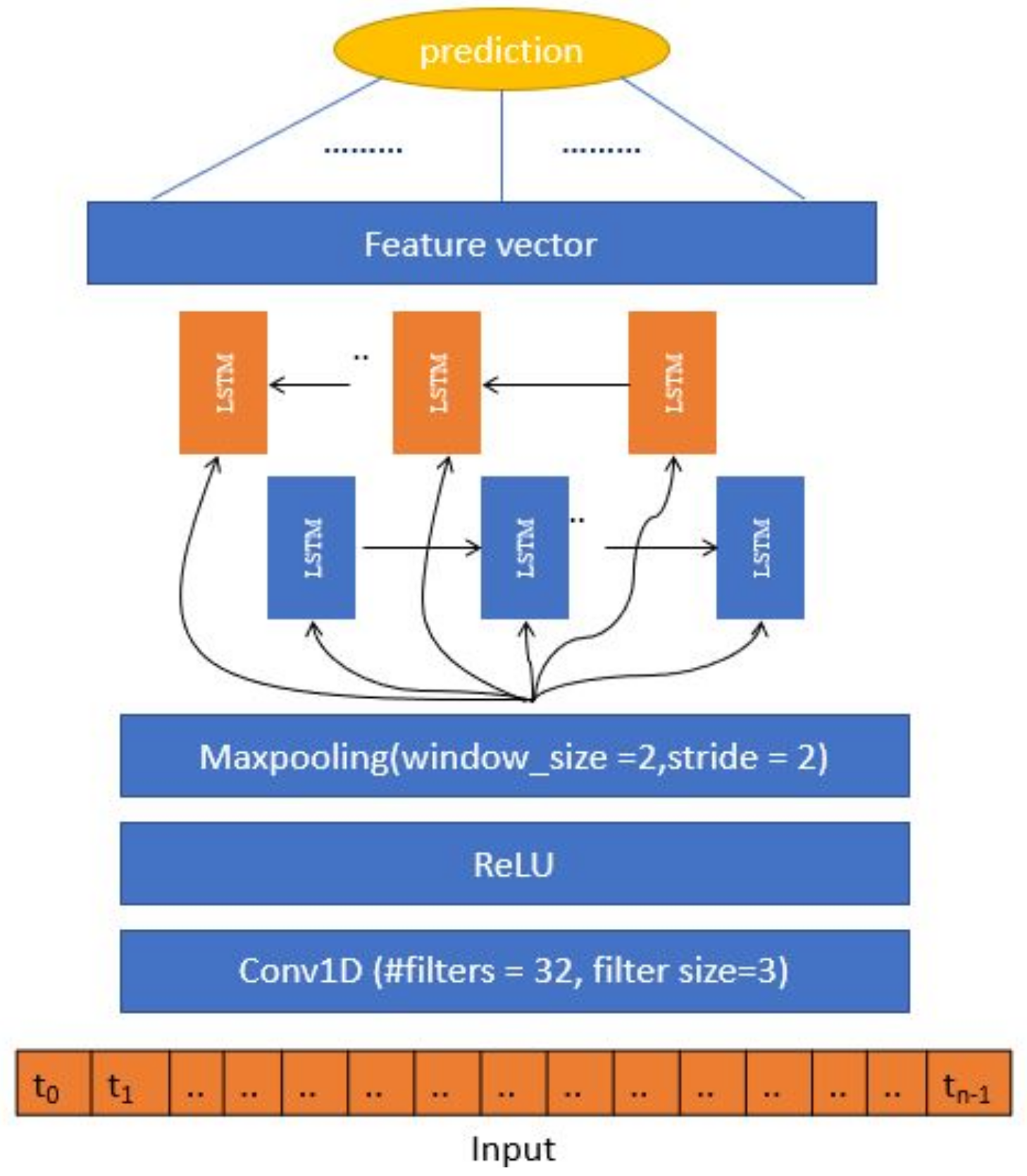
RNN is another typical deep learning model that is mainly used in natural language processing and speech recognition [31,32]. It is used to understand the data’s sequential behavior and predict the next likely outcomes [33]. In this paper, we have used a one bidirectional long short-term memory (LSTM) layer with 16 nodes followed by a dropout layer [34] with a dropout probability of 0.2, and a fully-connected layer with one node for prediction. Figure 4 shows the architecture of the RNN model. Bi-LSTM has been used in different areas such as phoneme classification [35], speech recognition [36], human action recognition [37], and machine translation [38]. Different gates are available in the LSTM cell. The input gate is used to decide which information should be stored for the next layer and update the current state. The forget gate is used to decide the information that should be removed according to the previous inputs. The output gate decides which part of the state value should be output. Thus, considering an input sequence {x} t = 1 T , the LSTM has cell states {C} t = 1 T , hidden states {h} t = 1 T and outputs a sequence {o} t = 1 T . This can be expressed mathematically by Equation (2) where W i , W o , W f , U i , U o , U f are the weight matrices and b o , b c , b i , b f are the biases. Sigmoid and Tanh are the activation functions. The ⊙ is the element-wise multiplication.
f t = σ ( b f + U f h t 1 + W f x t ) i t = σ ( b i + U i h t 1 + W i x t ) c t = i t t a n h ( b c + U c h t 1 + W c x t ) + f t c t 1 o t = σ ( b o + U o o t 1 + W o x t ) h t = o t t a n h ( c t )
In addition, we have designed a hybrid model for future demand prediction. This model consists of a 1-d convolution layer of 32 filters with a filter size of 3, ReLU, and a max-pooling layer. Then a bidirectional LSTM layer with 16 nodes. The learned features from the hybrid model are then fed into the fully connected layer with 1 node for prediction. This model is shown in Figure 5.
For all of these models, we used the grid search algorithm for hyper-parameters tuning. We used Keras framework for building and training the proposed models (https://keras.io/). The number of the epochs was set to 40 with early stopping based on validation loss. The RMSprop optimizer was used for optimization with learning rate of 0.001 [39].

3. Results and Discussions

In this paper, we used mean absolute error (MAE) and R 2 in order to evaluate the performance of the proposed models. These parameters were calculated using the Scikit-learn tool (https://scikit-learn.org/stable/).
We predicted future demands of facility capacity, supply capacity, and power consumption. We tested the three developed tools namely CNN, RNN, and the hybrid model using different values of histories and futures. Table 2 shows the best performing model with its past and future configurations for the three features of the study. The ’-’ sign in Table 2 means that the model did not fit the data at all. CNN model significantly outperforms RNN and hybrid models. We have extensively searched for the best hyperparameters and architectures of RNN models but these models did not converge. The main reason is that the size of the training dataset is not large enough to train the RNN model. Thus, our future work will concentrate on collecting more data from Korean Power Exchange to train more accurate forecasting models. Therefore, we will consider the CNN model for power demands forecasting.
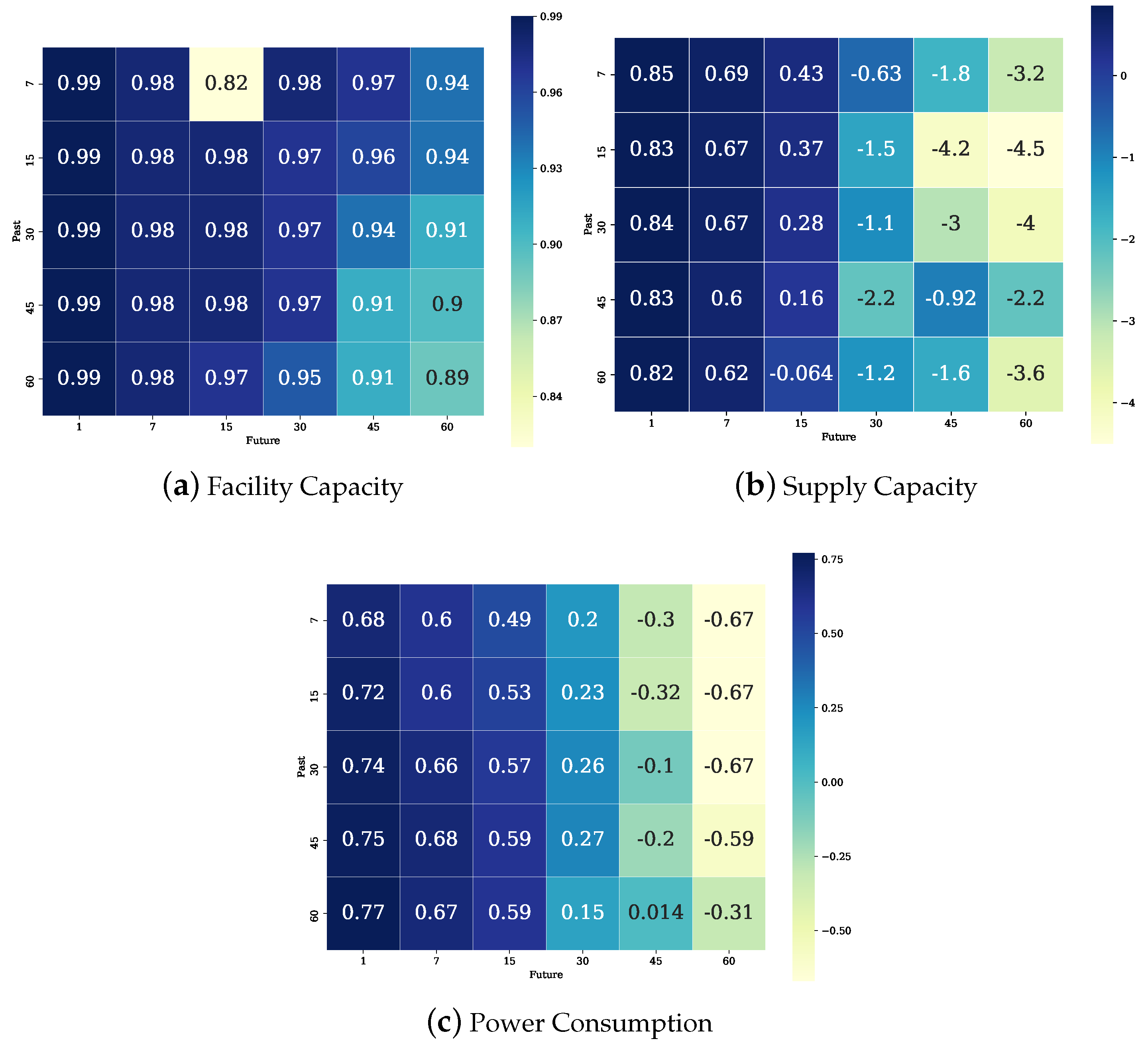
Figure 6 shows the heat maps of the R 2 results for all past against future configurations in the CNN model. For facility capacity forecasting, we can see that the CNN model performs outstandingly for all combinations. The best R 2 value is 0.992 for the past of 7 days and the future of 1 day. On the other hand the minimum R 2 is 0.820 for the past of 7 days and the future of 15 days. Thus, we can use the developed CNN model for facility capacity forecasting using different past values for predicting different future values.
For supply capacity forecasting, we can see that the CNN model performs well for some combinations only, forecasting up to 15 days. The best R 2 value is 0.851 for the past of 7 days and the future of 1 day. Thus, we can use the developed model for short-term forecasting. The model can forecast with 0.69 of R 2 for the past of 7 days and the future of 7 days. Furthermore, the R 2 is 0.43 for the past of 7 days and the future of 15 days.
For power consumption forecasting, we can see that the CNN model performs well for some combinations only. The best R 2 value is 0.772 for the past of 60 days and the future of 1 day. Thus, we can use the developed model for short-term forecasting. The model can forecast with 0.68 of R 2 for the past of 45 days and the future of 7 days. Furthermore, the R 2 is 0.59 for the past of 45 or 60 days and the future of 15 days.
Furthermore, the MAE of the CNN model outperforms the MAE results of the other models. For instance, the MAE of facility capacity feature is 0.025. On other hand, the MAE of the supply capacity of the CNN model is better by 0.265 than the hybrid model. Similarly, the MAE of the CNN model in power consumption features is better by 0.095 of the hybrid model.
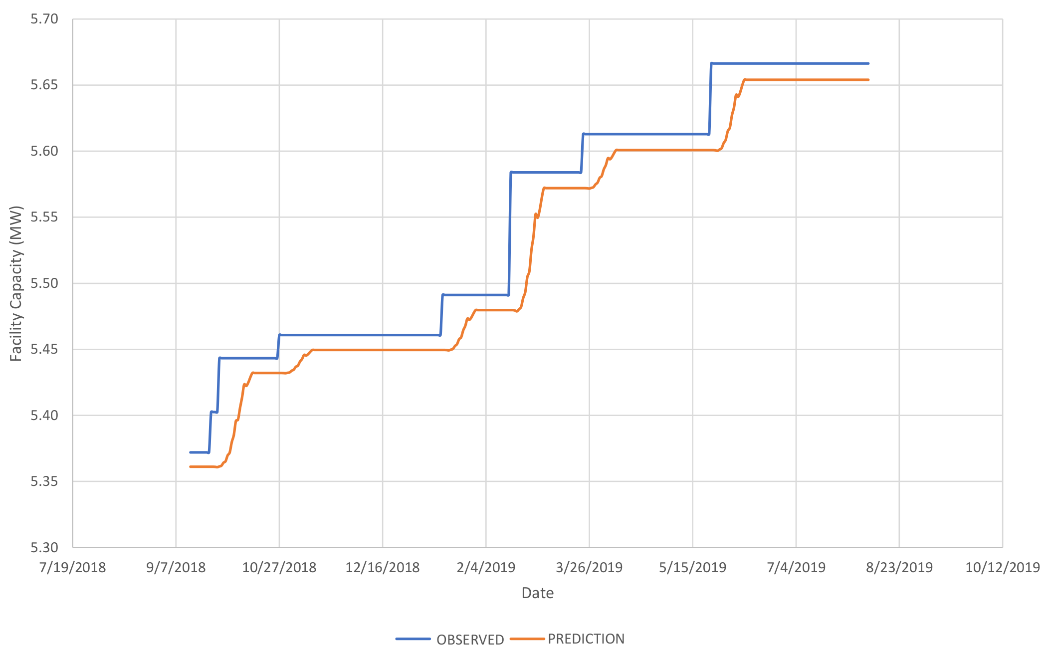
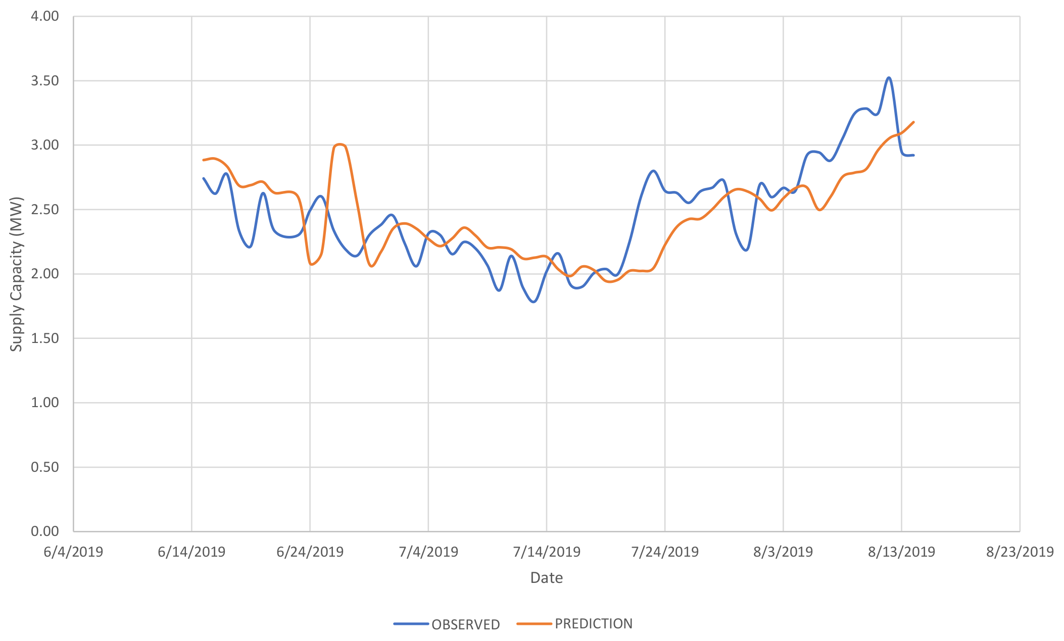
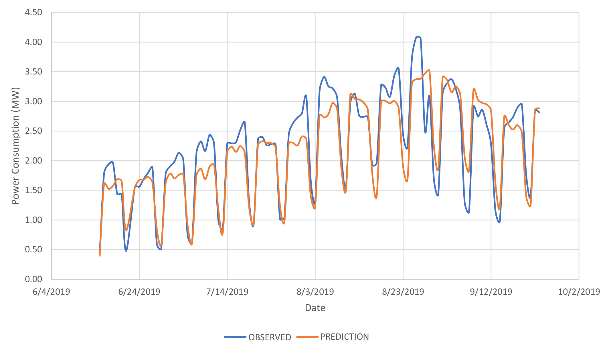
In addition, we visualize the performance of CNN model for the three features in a sample future interval as shown in Figure 7, Figure 8 and Figure 9, respectively. It can be seen that the predicted results of facility capacity and power consumption follow the observed values. On the other hand, the predicted results of supply capacity are not always following the observed trend.
In order to see the real performance of the proposed model, we compared it with a support vector machine (SVM) and artificial neural networks (ANN). SVM was chosen as a benchmark model because previous researchers have proven that SVM can produce satisfactory performance across various power demands forecasting [40,41,42]. For a fair comparison, we also performed a hyperparameter search for the penalty factor and gamma using grid search and found that the best performing penalty factor and gamma are 1 and 0.001 for the facility capacity feature, 0.001 and 1 for the supply capacity feature, and 100 and 0.001 for the power consumption feature.
ANN models have been used by many researchers and showed good performance such as [10,14,15]. We have also performed a grid search for hyperparameter optimization. We designed a two-layer ANN model where the first layer has 32 nodes followed by ReLU as a non-linear activation function. Then a dropout layer with a drop rate of 0.5 was added. The second layer has one node for prediction. Table 3 shows the comparison results between the proposed model and SVM and ANN models. It can be seen that the CNN model outperforms ANN and SVM in facility capacity and supply capacity features. However, in power consumption, SVM performs slightly better. It is known that deep learning models require big datasets for training them therefore, our future work will include collecting large datasets for more accurate forecasting models.

4. Conclusions

Power demands forecasting is a challenging topic and important for future planning. In this paper, we introduced the utilization of different deep learning models for future demands forecasting for facility capacity, supply capacity, and power consumption. Different deep learning architectures were studied, namely CNN, RNN, and the hybrid model that combines CNN with RNN. The experimental results show that the CNN model outperformed RNN and hybrid model significantly. Furthermore, we compared the performance of the CNN model with SVM and ANN models. The comparison results showed that CNN performs generally better. The developed CNN model is a short-term power demand forecasting model as it cannot forecast more than one day. The future plan is collecting more training data from the Korea Power Exchange in order to train a more robust forecasting model that can perform mid-term to long-term power demand forecasting.

Author Contributions

T.K. and D.Y.L. and H.T. prepared the dataset, conceived the algorithm, and carried out the experiment and analysis. T.K., D.Y.L., and H.T. wrote the manuscript with support from K.T.C. All authors discussed the results and contributed to the final manuscript. All authors have read and agreed to the published version of the manuscript.

Funding

National Research Foundation of Korea: 2020R1A2C2005612; National Research Foundation of Korea: NRF-2017M3C7A1044816.

Acknowledgments

This work was supported in part by the National Research Foundation of Korea (NRF) grant funded by the Korea government (MSIT) (No. 2020R1A2C2005612), in part by the Brain Research Program of the National Research Foundation (NRF) funded by the Korean government (MSIT) (No. NRF-2017M3C7A1044816), and in part by Basic Science Research Program through the National Research Foundation of Korea (NRF) funded by the Ministry of Education (No. 2019R1A6A3A01094685).

Conflicts of Interest

The authors declare that they have no competing interests.

References

  1. Al-Shakarchi, R.G.; MM Ghulaim, M. Short-term load forecasting for baghdad electricity region. Electr. Mach. Power Syst. 2000, 28, 355–371. [Google Scholar]
  2. Sadeghi, K.; Ghaderi, S.; Azadeh, A.; Razmi, J. Forecasting electricity consumption by clustering data in order to decrease the periodic variable’s effects and by simplifying the pattern. Energy Convers. Manag. 2009, 50, 829–836. [Google Scholar] [CrossRef]
  3. Alfares, H.K.; Nazeeruddin, M. Electric load forecasting: Literature survey and classification of methods. Int. J. Syst. Sci. 2002, 33, 23–34. [Google Scholar] [CrossRef]
  4. Pedregal, D.J.; Trapero, J.R. Mid-term hourly electricity forecasting based on a multi-rate approach. Energy Convers. Manag. 2010, 51, 105–111. [Google Scholar] [CrossRef]
  5. Weron, R. Modeling and Forecasting Electricity Loads and Prices: A Statistical Approach; John Wiley & Sons Ltd.: West Sussex, UK, 2007; Volume 403. [Google Scholar]
  6. Hu, H.; Wang, L.; Peng, L.; Zeng, Y.R. Effective energy consumption forecasting using enhanced bagged echo state network. Energy 2020, 193, 116778. [Google Scholar] [CrossRef]
  7. Chen, G.; Li, K.; Chung, T.; Sun, H.; Tang, G. Application of an innovative combined forecasting method in power system load forecasting. Electr. Power Syst. Res. 2001, 59, 131–137. [Google Scholar] [CrossRef]
  8. Álvarez, C.; Añó, S. Stochastic load modelling for electric energy distribution applications. Top 1994, 2, 151–166. [Google Scholar] [CrossRef]
  9. De Gooijer, J.G.; Hyndman, R.J. 25 years of time series forecasting. Int. J. Forecast. 2006, 22, 443–473. [Google Scholar] [CrossRef] [Green Version]
  10. Ediger, V.Ş.; Akar, S. ARIMA forecasting of primary energy demand by fuel in Turkey. Energy Policy 2007, 35, 1701–1708. [Google Scholar] [CrossRef]
  11. Chen, H.; Canizares, C.A.; Singh, A. ANN-based short-term load forecasting in electricity markets. In Proceedings of the 2001 IEEE Power Engineering Society Winter Meeting (Cat. No. 01CH37194), Columbus, OH, USA, 28 January–1 February 2001; Volume 2, pp. 411–415. [Google Scholar]
  12. Hahn, H.; Meyer-Nieberg, S.; Pickl, S. Electric load forecasting methods: Tools for decision making. Eur. J. Oper. Res. 2009, 199, 902–907. [Google Scholar] [CrossRef]
  13. Niu, D.X.; Wang, Q.; Li, J.C. Short term load forecasting model based on support vector machine. In Advances in Machine Learning and Cybernetics; Springer: Guangzhou, China, 2006; pp. 880–888. [Google Scholar]
  14. Martín-Merino, M.; Román, J. A new SOM algorithm for electricity load forecasting. In International Conference on Neural Information Processing; Springer: Hong Kong, China, 2006; pp. 995–1003. [Google Scholar]
  15. Metaxiotis, K.; Kagiannas, A.; Askounis, D.; Psarras, J. Artificial intelligence in short term electric load forecasting: A state-of-the-art survey for the researcher. Energy Convers. Manag. 2003, 44, 1525–1534. [Google Scholar] [CrossRef]
  16. Liu, K.; Subbarayan, S.; Shoults, R.; Manry, M.; Kwan, C.; Lewis, F.; Naccarino, J. Comparison of very short-term load forecasting techniques. IEEE Trans. Power Syst. 1996, 11, 877–882. [Google Scholar] [CrossRef]
  17. Bo, H.; Nie, Y.; Wang, J. Electric load forecasting use a novelty hybrid model on the basic of data preprocessing technique and multi-objective optimization algorithm. IEEE Access 2020, 8, 13858–13874. [Google Scholar] [CrossRef]
  18. Hippert, H.S.; Pedreira, C.E.; Souza, R.C. Neural networks for short-term load forecasting: A review and evaluation. IEEE Trans. Power Syst. 2001, 16, 44–55. [Google Scholar] [CrossRef]
  19. Gonzalez-Romera, E.; Jaramillo-Moran, M.A.; Carmona-Fernandez, D. Monthly electric energy demand forecasting based on trend extraction. IEEE Trans. Power Syst. 2006, 21, 1946–1953. [Google Scholar] [CrossRef]
  20. Srinivasan, D.; Lee, M. Survey of hybrid fuzzy neural approaches to electric load forecasting. In Proceedings of the 1995 IEEE International Conference on Systems, Man and Cybernetics. Intelligent Systems for the 21st Century, Yokohama, Japan, 20–24 March 1995; Volume 5, pp. 4004–4008. [Google Scholar]
  21. Beccali, M.; Cellura, M.; Brano, V.L.; Marvuglia, A. Forecasting daily urban electric load profiles using artificial neural networks. Energy Convers. Manag. 2004, 45, 2879–2900. [Google Scholar] [CrossRef]
  22. Berriel, R.F.; Lopes, A.T.; Rodrigues, A.; Varejao, F.M.; Oliveira-Santos, T. Monthly energy consumption forecast: A deep learning approach. In Proceedings of the 2017 International Joint Conference on Neural Networks (IJCNN), Anchorage, AK, USA, 14–19 May 2017; pp. 4283–4290. [Google Scholar]
  23. Chandramitasari, W.; Kurniawan, B.; Fujimura, S. Building deep neural network model for short term electricity consumption forecasting. In Proceedings of the 2018 International Symposium on Advanced Intelligent Informatics (SAIN), Yogyakarta, Indonesia, 29 August 2018; pp. 43–48. [Google Scholar]
  24. Nair, A.S.; Hossen, T.; Campion, M.; Ranganathan, P. Optimal operation of residential EVs using DNN and clustering based energy forecast. In Proceedings of the 2018 North American Power Symposium (NAPS), Fargo, ND, USA, 9–11 September 2018; pp. 1–6. [Google Scholar]
  25. Balaji, A.J.; Harish Ram, D.; Nair, B.B. A deep learning approach to electric energy consumption modeling. J. Intell. Fuzzy Syst. 2019, 36, 4049–4055. [Google Scholar] [CrossRef]
  26. Bedi, J.; Toshniwal, D. Deep learning framework to forecast electricity demand. Appl. Energy 2019, 238, 1312–1326. [Google Scholar] [CrossRef]
  27. Kim, T.Y.; Cho, S.B. Predicting residential energy consumption using CNN-LSTM neural networks. Energy 2019, 182, 72–81. [Google Scholar] [CrossRef]
  28. Oğcu, G.; Demirel, O.F.; Zaim, S. Forecasting electricity consumption with neural networks and support vector regression. Procedia-Soc. Behav. Sci. 2012, 58, 1576–1585. [Google Scholar] [CrossRef] [Green Version]
  29. LeCun, Y.; Bottou, L.; Bengio, Y.; Haffner, P. Gradient-based learning applied to document recognition. Proc. IEEE 1998, 86, 2278–2324. [Google Scholar] [CrossRef] [Green Version]
  30. Hochreiter, S.; Schmidhuber, J. Long short-term memory. Neural Comput. 1997, 9, 1735–1780. [Google Scholar] [CrossRef] [PubMed]
  31. Sutskever, I.; Vinyals, O.; Le, Q.V. Sequence to sequence learning with neural networks. In Advances in Neural Information Processing Systems; Curran Associates, Inc.: Montreal, QC, Canada, 2014; pp. 3104–3112. [Google Scholar]
  32. Yao, K.; Zweig, G. Sequence-to-sequence neural net models for grapheme-to-phoneme conversion. arXiv 2015, arXiv:1506.00196. [Google Scholar]
  33. Wang, Y.; Long, M.; Wang, J.; Gao, Z.; Philip, S.Y. Predrnn: Recurrent neural networks for predictive learning using spatiotemporal lstms. In Advances in Neural Information Processing Systems; Curran Associates, Inc.: Long Beach, CA, USA, 2017; pp. 879–888. [Google Scholar]
  34. Srivastava, N.; Hinton, G.; Krizhevsky, A.; Sutskever, I.; Salakhutdinov, R. Dropout: A simple way to prevent neural networks from overfitting. J. Mach. Learn. Res. 2014, 15, 1929–1958. [Google Scholar]
  35. Graves, A.; Schmidhuber, J. Framewise phoneme classification with bidirectional LSTM and other neural network architectures. Neural Netw. 2005, 18, 602–610. [Google Scholar] [CrossRef] [PubMed]
  36. Graves, A.; Jaitly, N.; Mohamed, A.R. Hybrid speech recognition with deep bidirectional LSTM. In Proceedings of the 2013 IEEE workshop on automatic speech recognition and understanding, Olomouc, Czech Republic, 8–12 December 2013; pp. 273–278. [Google Scholar]
  37. Zhu, W.; Lan, C.; Xing, J.; Zeng, W.; Li, Y.; Shen, L.; Xie, X. Co-occurrence feature learning for skeleton based action recognition using regularized deep LSTM networks. arXiv 2016, arXiv:1603.07772. [Google Scholar]
  38. Sundermeyer, M.; Alkhouli, T.; Wuebker, J.; Ney, H. Translation modeling with bidirectional recurrent neural networks. In Proceedings of the 2014 Conference on Empirical Methods in Natural Language Processing (EMNLP), Doha, Qatar, 25–29 October 2014; pp. 14–25. [Google Scholar]
  39. Tieleman, T.; Hinton, G. Lecture 6.5—RMSProp. In COURSERA: Neural Networks for Machine Learning; Report; University of Toronto: Toronto, ON, Canada, 2012. [Google Scholar]
  40. Son, H.; Kim, C. Short-term forecasting of electricity demand for the residential sector using weather and social variables. Resour. Conserv. Recycl. 2017, 123, 200–207. [Google Scholar] [CrossRef]
  41. Chen, Y.; Xu, P.; Chu, Y.; Li, W.; Wu, Y.; Ni, L.; Bao, Y.; Wang, K. Short-term electrical load forecasting using the Support Vector Regression (SVR) model to calculate the demand response baseline for office buildings. Appl. Energy 2017, 195, 659–670. [Google Scholar] [CrossRef]
  42. Khosravi, A.; Koury, R.; Machado, L.; Pabon, J. Prediction of hourly solar radiation in Abu Musa Island using machine learning algorithms. J. Clean. Prod. 2018, 176, 63–75. [Google Scholar] [CrossRef]
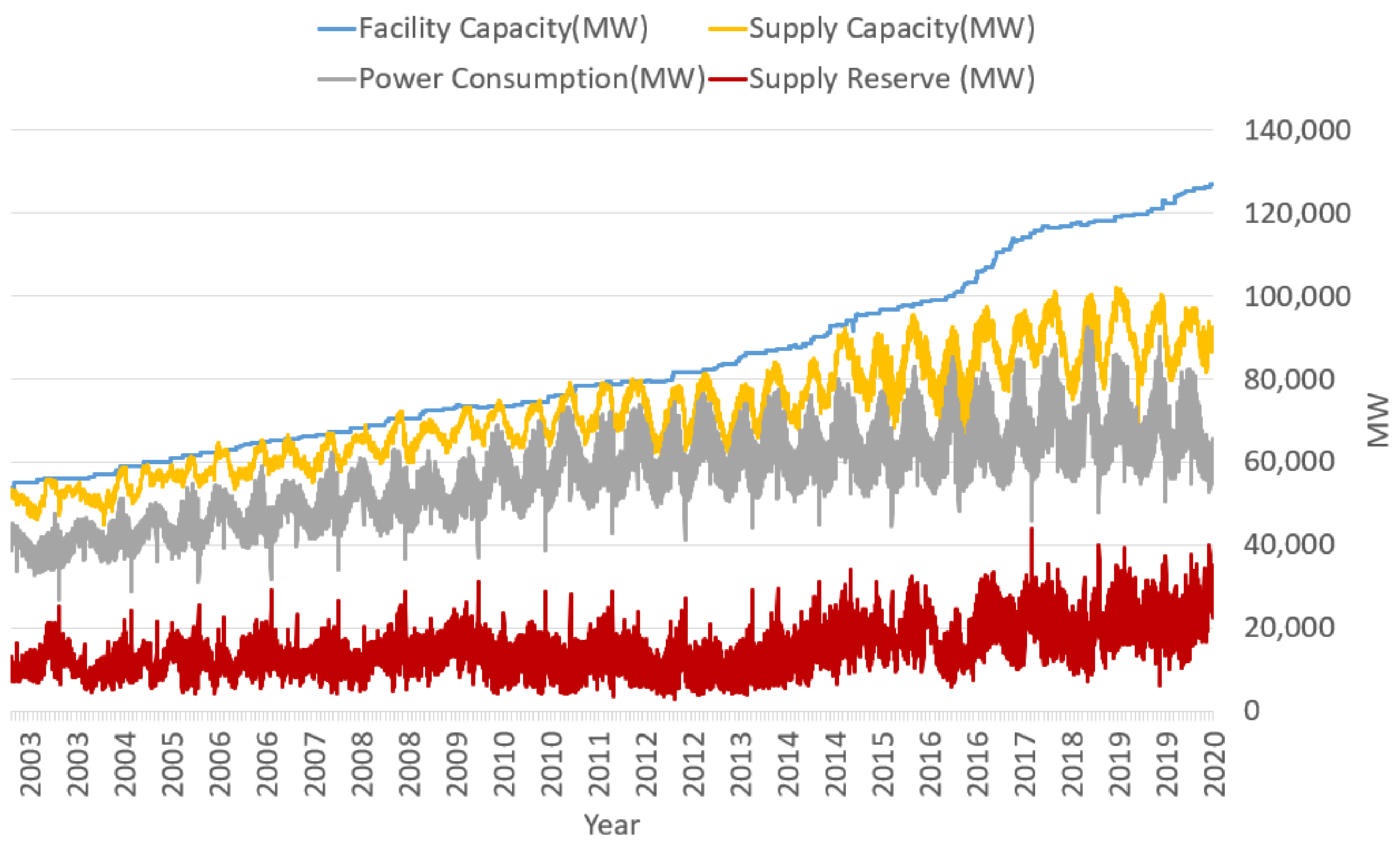
Figure 1. The characteristics of the features in the dataset within the period of the study.
Applsci 10 07241 g001
Figure 2. Example of data preparation.
Applsci 10 07241 g002
Figure 3. The architecture of the convultional neural network (CNN) model.
Applsci 10 07241 g003
Figure 4. The architecture of the recurrent neural network (RNN) model.
Applsci 10 07241 g004
Figure 5. The architecture of the hybrid model.
Applsci 10 07241 g005
Figure 6. The heat map of R 2 results for different past and future configurations in the CNN model.
Applsci 10 07241 g006
Figure 7. An example of the facility capacity prediction performance of the CNN model.
Applsci 10 07241 g007
Figure 8. An example of the supply capacity prediction performance of the CNN model.
Applsci 10 07241 g008
Figure 9. An example of the power consumption prediction performance of the CNN model.
Applsci 10 07241 g009
Table 1. The statistical overview of facility capacity, supply capacity, and power consumption.
FeatureCountMeanSTDMinimum Value (MW)Maximum Value (MW)
Facility Capacity (MW)6352.083,447.0320,918.8253,800.0126,887.0
Supply Capacity (MW)6352.072,243.5813,245.4544,937.0101,923.0
Power Consumption (MW)6352.058,550.0611,468.3226,916.092,478.0
Table 2. The best performance of the proposed models with different past and future configurations.
FeatureModelPast (days)Future (days)R 2 MAE
Facility Capacity (MW)CNN710.9920.025
Supply Capacity (MW) 710.8510.214
Power Consumption (MW) 6010.7720.314
Facility Capacity (MW)RNN----
Supply Capacity (MW) ----
Power Consumption (MW) ----
Facility Capacity (MW)Hybrid (CNN+RNN)----
Supply Capacity (MW) 6010.3360.479
Power Consumption (MW) 710.6270.409
Table 3. Performance comparison between the proposed model and support vector machine (SVM) and artificial neural networks (ANN) in terms of mean absolute error (MAE).
FeatureCNNANNSVM
Facility Capacity (MW)0.0250.5021.285
Supply Capacity (MW)0.2140.2623.218
Power Consumption (MW)0.3140.3980.308
Publisher’s Note: MDPI stays neutral with regard to jurisdictional claims in published maps and institutional affiliations.