Abstract
High-accuracy determination of a microseismic (MS) location is the core task in MS monitoring. In this study, a 3D multi-scale grid Green’s function database, depending on recording wavefield frequency band for the target mining area, is pre-generated based on the reciprocity theorem and 3D spectral element method (SEM). Then, a multi-scale global grid search strategy is performed based on this pre-stored Green’s function database, which can be effectively and hierarchically processed by searching for the spatial location. Numerical wavefield modeling by SEM effectively overcomes difficulties in traditional and simplified ray tracing modeling, such as difficult wavefield amplitude and multi-path modeling in 3D focusing and defusing velocity regions. In addition, as a key step for broadband waveform simulation, the source-time function estimated from a new data-driven singular value decomposition averaged fractional derivative based wavelet function (DD-SVD-FD wavelet) was proposed to generate high-precision synthetic waveforms for better fitting observed broadband waveform than those by simple and traditional source-time function. Combining these sophisticated processing procedures, a new robust grid search and waveform inversion-based location (GSWI location) approach is integrated. In the synthetic test, we discuss and demonstrate the importance of 3D velocity model accuracy to waveform inversion-based location results for a practical MS monitoring configuration. Furthermore, the average location error of the 3D GSWI location for eight real blasting events is only 15.0 m, which is smaller than error from 3D ray tracing-based location (26.2 m) under the same velocity model. These synthetic and field application investigations prove the crucial role of 3D velocity model, finite-frequency travel-time sensitivity kernel characteristics and accurate numerical 3D broadband wavefield modeling for successful MS location in a strong heterogeneous velocity model that are induced by the presence of ore body, host rocks, complex tunnels, and large excavations.
1. Introduction
Mine microseismic (MS) monitoring can effectively evaluate the risks of a mining area and optimize production plan, in which MS location is a fundamental indicator parameter to study the fracturing location of rock mass, understand crack extension law, focal mechanism inversion, and analyze characteristics of mining activities [1,2,3]. At present, ray tracing-based location methods based on travel time are generally used for MS location, in which the objective function is built by the difference between theoretical and picked arrival time of specified seismic phases. The ray tracing-based location methods have been widely used in the literature due to their simple theory and operation. Detailed reviews of related studies can refer to [4,5]. However, ray tracing-based location methods are set up on the basis of geometrical ray approximation for high-frequency wave propagating, which have inherent difficulties in modeling multi-path effects and focusing and defocusing effects of realistic broadband wavefield propagation in complex velocity structure. Moreover, they could be easily affected by large arrival time picking errors. The above shortcomings increase difficulties in an accurate location with ray tracing-based location technique [6]. In the past few years, with the development of computer technologies and improvement of numerical modeling methods, wave equation-based location methods have been gradually introduced and applied to a MS location in the fields of mining and oil-gas exploration. Wave equation-based modeling can overcome the above shortcomings of simplified ray tracing-based location methods. In addition, the wave equation-based location can directly utilize the recording broadband waveform data, that is, it does not require the high-accuracy arrival time picking of specified seismic phase. Wave equation-based location methods usually fall into two categories, i.e., wavefield reverse-time migration-based location [7] and waveform inversion-based location [8]. The former takes the maximum energy spatial point of stacking backpropagated waveform from all sensors as the location result, and it only requires a small amount of simultaneous wavefield simulations. For example, Witten and Shragge [9,10] developed a full wavefield-based reverse time imaging method for locating microseismic events. The wavefield reverse-time migration-based location methods are conceptually simple and easy to perform, but the critical imaging conditions for location can be easily affected by noises [11]. As the ultimate means of geophysical inversion, waveform inversion-based location methods takes advantage of the fitting degree between synthetic waveforms and observed waveforms, which fully considers waveform complexity and can comprehensively constrain the source location.
1.1. Calculation of the Green’s Function
A high accuracy Green’s function is the basis for a successful waveform inversion (see Section 2.1 for more details). Due to limited computing resources in the early years, the frequency wavenumber (FK) method that adopts a one-dimensional (1D) horizontal layered velocity model was usually used to model Green’s function. Moreover, Tkalčić et al. [12] utilized different 1D velocity models from the source to each station to reduce the influence of velocity models errors. However, in complex structural areas including mines, there is strong three-dimensional (3D) heterogeneity, thus, a 1D velocity model usually cannot accurately model broadband seismic waveforms in such regions. In particular, it performs unsatisfactorily in characterizing the high frequency waveform information.
In recent years, with the improvement of parallel computing capabilities, the Green’s function numerical computation based on 3D velocity model (3D Green’s function) has been efficiently developed. Hsu et al. [13], Zeng and Song [14], Eisner and Clayton [15], Bignardi et al. [16] and Zhao et al. [17] separately modeled 3D Green’s functions by utilizing finite element method (FEM), finite difference method (FDM), boundary element method (BEM) and pseudo spectral method (PSM). However, the FEM is usually based on low-order polynomials that have poor performance in modeling high-frequency signals. The FDM is easy for implementation and has high calculation efficiency, but the FDM is hard to adapt to complex geological structures and irregular boundary conditions for preset numerical accuracy. The BEM can effectively deal with complex boundary problems, but it is often limited to simulate linear wavefield response in relatively simple media. The PSM has a very high calculation precision, but it is also difficult to handle complex regions and interfaces [18]. The spectral element method (SEM), combining the high accuracy of spectral methods and flexibility in grid generation of FEM, is becoming more and more popular in simulating broadband seismic wavefields in 3D complex structures. Komatitsch and Vilotte [19] and Komatitsch et al. [20] developed open source parallel programs (1D~3D SEMs) for modeling seismic waveforms. On this basis, Fichtner et al. [21] and Tape et al. [22] conducted the 3D SEM for imaging large-scale 3D velocity structures. While Liu et al. [23], Hejrani et al. [24] and Hejrani and Tkalčić [25] obtained focal mechanisms and locations of natural earthquakes in large-scale regions through the 3D SEM and full waveform inversion (FWI). In conclusion, 3D SEM-based waveform inversions have been successfully applied in imaging large-scale velocity structures, and inversions of focal mechanisms and source location for natural earthquakes. Inspired by this, we attempted to introduce the 3D SEM into broadband waveform modeling and source location in a mine, which has a smaller spatial scale but with more complex structures.
1.2. Waveform Inversion-Based Location Methods
Waveform inversion-based location methods constantly update synthetic waveforms by changing input source parameter models, and the source location is determined when the synthetic and observed waveforms have the best fitting. As early as 1982, McMechan [26] numerically modeled wavefield propagation in a two-dimensional (2D) uniform-velocity model using the FDM, and he inverted the source location and origin time of MS events. Then, Wu and McMechan [27] inverted source location and magnitude based on a more efficient PSM and approximate linear iterative algorithm. Sen et al. [28] developed a 1D velocity model and waveform fitting-based full moment tensor inversion and source location method, which has been applied to microseismic event location in the fields of mining engineering [29] and gas injection [30]. Michel and Tsvankin [31] simultaneously obtained the source location, origin time and point source moment tensor in a 2D inhomogeneous velocity model by the utilizing waveform inversion method. In addition, Michel and Tsvankin [32] and Igonin and Innanen [33] used waveform inversion to jointly inverse the microseismic event location and velocity model. Wang and Alkhalifah [34] put forward a source function independent waveform inversion to obtain a microseismic source location, origin time, and velocity model. Kim et al. [8], Rodriguez et al. [35], and Hejrani et al. [24,25] performed joint inversion on point source moment tensor and location for natural earthquakes in regional scales under high-resolution 3D velocity models. Multi-parameter joint inversion greatly increases the search dimensions and the nonlinearity of the waveform inversion problem, and the multi-parameters are essentially highly coupled in the inversion process, which make the nonlinear waveform inversion difficult to converge. Therefore, more search times or iteration numbers are needed to find the global optimal location.
Therefore, some studies have simplified the source parameter model into an inversion that only considers source locations (the simplification process and description are shown in Section 2.1), which improves inversion speed and reduces the nonlinearity of convergence. Shekar and Sethi [36] formulated an FWI scheme for determining hydraulic fracturing and mining microseismic event locations, and synthetic test on the 2-D SEG/EAGE overthrust model demonstrates its feasibility. Tong et al. [37] derived a waveform inversion-based location method using the time-domain wave equation and cross-correlation travel time measurement between simulated and observed waveform as the misfit. They tested the proposed location algorithm through 2D and 2.5D (a 2D velocity model is adopted in the vertical plane determined by the source location and sensor location) field and regional velocity models. While Huang et al. [38,39] derived a waveform inversion-based location method that is independent from source-time characteristics, and they successfully applied the fast convergent truncated Newton method for microseismic source location based on 2D and 3D velocity models. Iteration-based optimization technique is often used in the above nonlinear waveform inversion-based location problem, which may be strongly affected by the initial model choice and cannot fully search the whole model space to obtain global convergence. In view of the above difficulties, we adopted the SEM for accurate wavefield modeling and global grid search idea from Hejrani et al. [24] for global source location. The difference is that a multi-scale grid generation and search strategy depending on recording waveform frequency content (the fine grid wavefield only stored near the active mining zones) was used in this study, which greatly reduces the computational time and storage for global grid search.
1.3. Green’s Function Database Generated Based on the Reciprocity Theorem
The general idea of global grid search and waveform inversion-based location (GSWI location) is to calculate the Green’s function from each candidate grid point to each sensor, and then the synthetic waveform can be obtained through the product of Green’s function, source-time function, and point source moment tensor. However, such a large number of wavefield modeling in a 3D space is impossible for existing parallel computing. An accurate and wise choice is to use the reciprocity theorem in elastic dynamics [40] for reducing the computation of Green’s functions. According to the time-space reciprocity of point source Green’s function between source point and sensor point, it only needs to set the sensor locations as virtual sources for wavefield modeling. In this way, the Green’s function of each point in the whole space is generated and stored as a database. The reciprocity theorem can significantly reduce the computation of waveform modeling with tens of thousands of candidate source grid points, and it will be easy to recalculate the Green’s function database for any updated velocity model.
Taking advantage of the reciprocity theorem, many researchers have carried out a series of studies on GSWI location. Bouchon [41] investigated the radiation mode of teleseismic body waves by wavefield modeling combining the reciprocity theorem and flat layer velocity model. Graves and Wald [42] generated a Green’s function database using the reciprocity theorem and found that the 3D velocity model can more accurately invert finite fault sources than the 1D velocity model. Eisner and Clayton [43,44] used the reciprocity theorem to simulate the response of 300 earthquakes to Southern California faults along with site and complicated wavefield propagation path effects in complex heterogeneous media. In some other studies, focal mechanisms, source location, and velocity model are jointly studied by utilizing the reciprocity theorem. Lee et al. [45] and Lu and Zhou [46] carried out lowpass filtered waveform inversion to focal mechanism solutions of Southern California and Lushan earthquakes, respectively, in which the 3D Green’s function database is generated by the reciprocity theorem. By utilizing the reciprocity theorem and grid search algorithm, Hejrani et al. [24] and Hejrani and Tkalčić [25] conducted high-resolution waveform inversion on focal mechanism solutions and locations of earthquakes in Papua New Guinea, the Solomon Islands, and Australia. The results show that the waveform inversion results based on 3D velocity models are improved compared with those obtained by 1D velocity model. The above source parameter studies almost focus on natural earthquakes at regional scales, and there are few applications in broadband waveform modeling and source parameter inversion in a local scale (e.g., in the mine region) with more complex tectonic settings. With the improvement of computation capability and quality of broadband seismic records, it has become an inevitable trend to comprehensively carry out the 3D GSWI location study in a mine.
1.4. What Will Be Objectives of This Work
In this study, we introduced 3D waveform inversion for mine microseismic event location and applied a multi-scale grid search algorithm based on global optimization into source location problem in a complex 3D local region (abbreviated as MS-GSWI location). Our main contributions and innovations are shown as follows:
- (1)
- The SEM was used to effectively generate high-accurate 3D Green’s function in a mine region with complex structures, which overcomes the difficulties of modeling multi-path effects and focusing and defocusing effects in ray tracing methods.
- (2)
- A 3D Green’s function database in the mine was efficiently generated by the reciprocity theorem and served as multi-scale grid-search strategy, which largely improves the computational efficiency of 3D GSWI location.
- (3)
- Both the data-driven SVD-averaged fractional derivative based wavelet function (DD-SVD-FD wavelet) obtained by windowed specified seismic phases and traditional fractional-order Gaussian wavelet can be used for estimating the source-time function to generate synthetic waveforms for waveform inversion well. By comparing them, waveforms synthesized by the DD-SVD-FD wavelet have a higher accuracy and more reasonable physical explanation.
- (4)
- Synthetic test results show that the accuracy of velocity model is important for waveform inversion-based location, and the average location error of eight blasting events is only 15.0 m. The location error is smaller than the 3D ray tracing-based location method (average location error 26.2 m) under the same 3D velocity model.
The rest of this research is arranged as follows: Section 2 introduces main theories including synthetic waveform modeling based on the reciprocity theorem, estimation of source-time function with DD-SVD-FD wavelet, waveform modeling considerations, and multi-scale grid search strategy. In Section 3, dependence of GSWI location results to the accuracy of velocity model is tested by using velocity models with different smoothing degrees. Section 4 further tests effectiveness of the 3D proposed MS-GSWI location method by eight blasting events with known locations and compares it with previous published location results. In Section 5, the critical issues of 3D Green’s function database modeling, estimation of source-time function, and effects of 3D velocity model on location accuracy are discussed. Section 6 makes summaries and puts forward prospects for future work.
2. Methodology
2.1. Synthetic Waveforms Based on the Reciprocity Theorem
The core mission of waveform inversion is to find synthetic waveforms that fit the recording waveforms as much as possible. For a mine MS location, it is usually reasonable to treat the event as a point-source, and the synthetic waveform from earthquake location to sensor location is set as . Solving the elastic wave equation is a precise way to simulate three-component synthetic waveform, however, it is quite hard to obtain a high-resolution elastic parameter model for our study zone (limited by sparse single-component sensor network and low signal-to-noise ratio records). Therefore, in this study, results are all based on the acoustic wave equation. The synthetic waveform data can be simplified and calculated by the following equation:
where, the Green’s function refers to the time-space point pulse displacement response excited at the earthquake location on the sensor location , which is determined by , and propagation media distribution; and represent the normalized source-time function and origin time of a MS event, respectively; characterizes the influences of source amplitude and focal mechanism.
Complicated focal mechanism (such as double-couple, explosion) could significantly affect the waveform through source-time function form. The double-couple component, in contrast to the non-double-couple components usually reflecting collapse or implosive events, is an important indicator of shear fracture for a microseismic event. Its impact on waveform records is complicated. However, the influence of the double-couple component is generally better reflected and quantified in the waveform recorded by multi-component monitoring network with a higher signal-to-noise ratio through the complex polarity distribution character. Considering that it is usually difficult to constrain the double-couple component under a mining monitoring network with sparse single-component sensors and low signal-to-noise ratio records, blasting events were selected for synthetic and application tests of the GSWI location method in the study, and so the scalar acoustic wave approximation is acceptable. Therefore, the source amplitude can be naturally incorporated into the source-time function S(t), thus, the source-time function characterizes moment release rate, strength property, and rupture evolution at the source location. The origin time of an MS event can be regarded as an overall time-shift of all the recording waveforms. It can be eliminated in the data preprocessing step [11], then the is shortened as for convenience and Equation (1) can be rewritten as Equation (2). The source-time function estimation strategy will be defined in Section 2.2. After determining the source-time function, our focus moves to an accurate and efficient modeling of the Green’s function .
Assuming that the wavefield modeling is carried out at a preset highest frequency of 100 Hz, and the average P wave velocity is set as 4500 m/s, then the shortest wavelength of modeled wavefield will be 45 m. According to the sampling conditions of accurate wavefield simulation described in Section 2.3: for an accurate SEM numerical simulation, each wavelength should contain at least 4.5 grids [47], that is, the grid length should be less than 10 m. By referring to the mining zone of the Yongshaba mine (details in Section 4.1), the dimension is about 3000 × 1000 × 500 m3, then the number of grids reaches 300 × 100 × 50 = 1,500,000. If the recording waveforms are fitted through forward modeling waveforms, the Green’s function at each candidate source grid point will be modeled in the GSWI with relatively large computation.
To solve this computational problem, it is necessary to store the Green’s function in wavefield modeling as the database. Only a small number of wavefield-forward modeling is carried out based on the reciprocity theorem, that is, the number of wavefield modeling is directly proportional to the number of sensors instead of all searching grid points as candidate source. There are usually 10~50 sensors in a mine MS monitoring system, thus, it is easy to obtain the Green’s function from each sensor as virtual source to each grid point. In accordance to the reciprocity theorem in scalar acoustic wave representation, Equation (2) can be rewritten as:
where, denotes the Green’s function from the sensor location to source location . In a practical application, coarse grids are used in the regions far away from the mining area, and fine grids are used in the regions near the active mining area (where MS and blasting events occur frequently in practice). The combination of coarse and fine grids greatly reduce modeling computation and storage space of Green’s function database, which is called the multi-scale strategy. It is also conducive to improve the grid-search speed in the GSWI process.
For the broadband waveform inversion-based location method, it needs to define a reasonable objective function to determine the fitting degree of the target observed waveform and theoretical modeling waveform. After that, inversion algorithm searches for the minimum value corresponding point as the source location. Due to the complex geological structures and velocity distribution in a mining area, the inversion problem will be highly nonlinear if the L2 norm misfit between the synthetic and observed waveforms is directly used as the objective function. This research utilized the L2 norm difference of cross-correlation travel time as the objective function of GSWI location study, which is more robust and linear for inversion problems. The cross-correlation function of two discrete waveform time series is defined as follows:
The cross-correlation travel time difference is determined by the maximum value of Equation (4) based on the first-order approximation, that is, where, , is the time window function of specified seismic phases in the interval [0 T]. Through the summation of cross-correlation travel time difference of all windowed waveforms, the target misfit function for waveform inversion location is shown as follows:
where, M represents the number of windowed waveforms for location.
Compared with the ray tracing methods where one can generate a distribution of locations assuming some uncertainty on the arrival picks, the waveform-based location method uses wavefield information with limited frequency band distribution. Many factors will affect the uncertainty of the final location result in a coupled way, such as the recording clock deviation between different sensors, error of velocity model, and spatial distribution of sensor array with respect to microseismic events. In this study, the spatial distribution characteristics of the misfit function around the GSWI location point are used to qualitatively evaluate the uncertainty of location parameters. More sophisticated quantitative uncertainty analysis for waveform-based location is based on second-order Hessian matrix with respect to a target misfit function, which will be an independent future work.
2.2. Source-Time Function Estimation
The source-time function absorbing origin time and event magnitude is usually estimated by the Gaussian and Ricker wavelet [8,37], which is calculated as follows:
where, is the time value corresponding to wavelet central time; denotes the controlled dominant frequency, which is related with specified sensor frequency response.
While Wang [48] proposed a kind of Gaussian family wavelet based on fractional-order derivatives, whose frequency domain form is expressed as follows:
where, stands for the fractional-order of time differential. The fractional-order Gaussian function can change fractional order and at the same time, thus, it has more freedom than the pure Gaussian or Ricker wavelet. However, for quite dissimilar waveform data, there are still some limitations in wavefield modeling using the two parameters (, ) fractional-order Gaussian function as source-time function. In order to further improve fitting performance for complex waveforms, we put forward a new approach to obtain the source-time function based on observed waveforms themselves, namely the DD-SVD-FD wavelet estimation. The detailed steps are shown as follows: firstly, each recording waveform containing the first half period of P-phase arrival is cut by the semiautomatic windowing method proposed by Wang et al. [6]: (1) A two passes, four-poles, 200 Hz lowpass Butterworth filter was conducted to the recorded signal. (2) We manually picked a rough time T1 before the P-phase arrival and a rough time T2 after the first peak amplitude; (3) The T2 is automatically extended to the next zero amplitude time T3; (4) The windowed waveform corresponds to the filtered time series in the time interval [T1, T3]. The waveforms are aligned based on the cross correlation time difference between different windowed waveforms. Then, the SVD average of windowed and aligned signals is taken as a basis function, where SVD is a classical signal processing approach based on coherence between different data traces. It can enhance the signal-to-noise ratio and suppress incoherent background noise [49]. The aligned and windowed data traces can be represented by a data matrix (dimension is M × N), with M traces and N time samples per trace (usually M < N). Assuming that the data matrix has a rank R < M, the SVD of is a orthogonal expansion of the data space:
where, is the ith nonzero singular value, and and are the corresponding left and right singular eigenvectors with dimensions M and N, respectively. The product is a (M × N) matrix with rank one. If the windowed dataset has a high degree of trace-to-trace coherence, then the most coherent or average trace can be constructed from the largest singular eigenvector with the largest eigenvalue. The SVD acts as a data-driven, lowpass filter by keeping the main character of the dataset and rejecting highly incoherent noises.
Finally, time scaling factor and fractional-order are introduced to estimate the frequency-time domain characteristics and obtain the source-time function in the frequency-time domain as (Equation (9)).
where, indicates the denoised time sequence of the rth windowed and aligned waveform at the time (r = 1, 2, ..., M, and i = k, k + 1, ..., k + N − 1), k represents the start point of the windowed waveform. and separately stand for the Fourier transforms of S(t) and , in which a is a scaling factor in time domain. The optimal source-time function can be estimated by updating the two parameters [u, a] searching for the maximum value of normalized cross-correlation coefficient between recording waveform and synthetic waveform modeled from corresponding source-time function.
2.3. Wavefield Modeling Based on Acoustic Wave Equation
Tong et al. [37] and Huang et al. [38] derived wavefield modeling and waveform inversion-based location methods, by taking advantage of numerically solving the acoustic wave equations in time domain and frequency domain, respectively, and this study will carry out wavefield modeling under the same framework. The scalar acoustic wave equation in frequency domain can be expressed as follows:
where, indicates the compressional P wave velocity at point in the medium; represents the frequency spectrum of the source-time function , usually showing complex spectrum characteristics.
Through a series of derivations (see [37] for more details), sensitivity kernels with respect to velocity model parameters for wavefield disturbance at a sensor caused by the source spatial location disturbance are obtained by using the popular adjoint method. On this basis, in accordance with the objective function defined by waveform cross-correlation travel time difference and sensitivity kernels, and disturbance of model parameters in the wavefield propagation space (especially in first Fresnel zone surrounding the main energy ray path) can be obtained.
where, K is the cross-correlation travel time sensitivity kernel and represents the P wave velocity perturbation at point .
where, is the adjoint wavefield in the media excited by a virtual adjoint source defined at the sensor (the detailed derivation refers to [37]). The sensitivity kernel of travel time has very complex intensity and spatial distribution, which reflects the frequency-dependent weighted influence of velocity perturbation in the Fresnel zone on the final travel time anomaly recorded by sensor. It reveals the nature of finite frequency effects in actual wavefield propagation.
2.4. Numerical Wavefield Modeling Conditions
The accuracy of wavefield modeling generally needs to meet two key numerical conditions: the Courant–Friedrichs–Lewy (CFL) condition and the least sampling number of grid points for shortest wavelength in wavefield modeling. The CFL condition satisfies the following inequality:
where, , and indicate the velocity model, grid size and time step for numerical modeling, respectively; is the Courant number, generally ranging from 0.3 to 0.5.
Seriani and Priolo [47] pointed out that for a high accurate modeling by SEM, the number of grid points in the shortest simulated wavelength should meet the following condition:
where, is the shortest period of frequency band based on target modeled wavefield, is the average grid size. represents the number of grid points in a single wavelength that can maintain the numerical simulation accuracy, and it is fixed at 5 in the SPECFEM3D program used for this study. As shown in Equation (13), the smaller the shortest period of modeled wavefield, the smaller the required grid dimension.
Based on the above conditions, we know that after determining the highest frequency of modeled wavefield, the average grid size can be determined through Equation (14) and time step for modeling is then limited by Equation (13). Equation (14) shows that when the highest frequency of modeled wavefield is doubled, the grid size in each dimension will be reduced to half of the original one, and the number of 3D grid points will become eight times of the original number. Equation (13) indicates that as the grid dimension is reduced by half, the time step for modeling that maintains the stability of the time scheme will also be decreased by half. Therefore, when the highest frequency of modeled wavefield is doubled, the wavefield calculation will be 16 times the original one. This is why we propose the multi-scale strategy (also corresponding to the multi-grid operation depending on wavefield frequency content) to reduce the storage requirements and the computational cost.
3. Synthetic Test
To test the proposed 3D GSWI location method, the 3D velocity model inverted through ray tracing tomography based on P wave travel-time data by Wang et al. [50] and shown in Section 4.1 was selected as the target velocity model. Moreover, velocity models with different smoothing scales were used to verify the importance of velocity model accuracy to the 3D GSWI location method. In this method, a 3D spatial Gaussian function has been used for smoothing the original high-resolution velocity model, and the standard deviation is used to define the length of smoothing scale. This different smoothing length approximately reflects the different resolution limit of the ray-based tomographic model obtained from transmission wave data with various signal frequency content [51], while high and low velocity anomalies that are incorrectly positioned may result in a large location error are not considered in this paper. That is, we only conducted a specific qualitative assessment to consider the influence of insufficient resolution of inverted velocity model on GSWI location errors. Velocity model 2D slices under different smoothing scales are shown in Figure 1a. The synthetic test was carried out using the premeasured locations (locations measured before the blasting events) of eight practical blasting events and their corresponding sensors (Table 1 in [6]), and the waveform dataset was generated by the unsmoothed target 3D velocity model with 120 Hz dominant frequency referring to the data spectrum analysis.
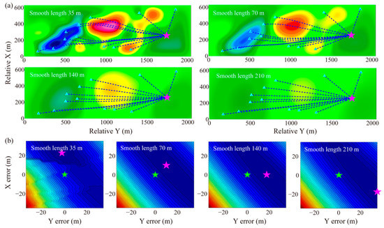
Figure 1.
Grid search and waveform inversion-based (GSWI) location results under different velocity model smoothing scales. (a) Velocity models under different smoothing scales and ray paths from source to each triggered sensor. The 2D slices of 3D tomographic velocity models showing here are determined by the summation least square of the vertical distances from all sensors. The backgrounds are the smoothed velocity models with smoothing lengths equaling to 35, 70, 140 and 210 m, respectively. The dotted lines show the ray tracing paths from the source location to corresponding triggered sensors. (b) Waveform misfit contour map of GSWI location result at grid points near the true source location for different smoothing scales. The smoothing lengths from left to right are 35, 70, 140, and 210 m, respectively. The pink star is the location determined by the GSWI location method, while the green star corresponds to the true event location.
The location of blasting event 8 is taken as the example and its waveform inversion-based location results are demonstrated in Figure 1. The figure shows that with the increase of smoothing lengths, the smoothed velocity models gradually tend to be homogeneously distributed, which are characterized by the ray paths from the source to each sensor that gradually become straight lines. The 17.5 m smoothing obtained a 0 m location error, as when a relatively accurate velocity model is used for location, the waveform information related to source location could still be reasonably explored and inverted by the grid search and waveform inversion-based location method. When the model error increases (the smoothing length continues to increase), the source information contained in the data cannot be inverted or stacked correctly, and the location error introduced by velocity error appears. Location errors caused by reduction of velocity model accuracy do not follow a monotonous change law, due to location result is also being controlled by some other factors, such as specific triggered sensor geometric distribution and inhomogeneity of velocity structures near the source location. Furthermore, the overall location error increases with the decrease of velocity model accuracy (Figure 2), which confirms the necessity of an accurate 3D velocity model to waveform inversion-based location in regions with complex geological structural property. In addition, the errors of GSWI location results in this synthetic test with a small number of test events are all within 40 m. It is complicated to perform a completely quantitative analysis explaining the coupling effect between the location error and the current velocity model inaccuracy (such as by smoothing). The systematic location error analysis will be left to the future.
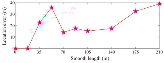
Figure 2.
GSWI location errors under different velocity model smoothing scales for the blasting event 8.
4. Application
4.1. Engineering Background and Multi-Scale Grid Generation
In this study, eight blasting events obtained by the MS monitoring system (Figure 3) in the Yongshaba mine (China) were selected for application test. In this system, there are 28 sensors: sensors T1 and T2 are triaxial sensors, sensors 1–26 are uniaxial sensors, and they are set at the 930 m level (12 sensors), 1080 m level (12 sensors), and 1120 m level (4 sensors) along the mining tunnels. The main working principles of the Institute of Mine Seismology (IMS) are shown as follows: firstly, a sensor can monitor the signal all the time. Then, the continuous signal is transported to its administering NetADC (network analogue-to-digital converter) through 4 core signal cable (uniaxial sensor) and 8 core signal cables (triaxial sensor), and the NetADC samples the signal 6000 times per second (it means that the sampling frequency of a microseismic signal that we used is 6000 Hz). After that, the NetSP (network seismological processor) does some pre-processing to the discrete signal, which comes from its administrated NetADC, including the detection of MS event signals based on threshold value. Finally, the detected discrete signal is transferred to the data exchange center, and then the data processing center. Based on microseismic signals, we can calculate microseismic event location, magnitude, focal mechanism, etc.
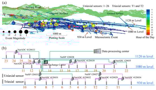
Figure 3.
Microseismic monitoring model and system structure diagram of the microseismic (MS) system installed at the Yongshaba mine. (a) Microseismic monitoring model modified from Li et al. [52]. The red fonts correspond to the sensor id, green grid means the ground surface, dark orange line is the Jinyang road, blue lines are different mining levels, and light blue lines are the mining levels with sensor distributed. The spheres are locations of microseismic events; (b) System structure diagram of the MS system modified from Shang et al. [53]. The green line represents 4 core optical fiber, pink line represents 4 core signal cable, and the bold pink line represents 8 core signal cable.
The dip angle of ore body in the mine was about 30°. The hanging wall of ore body is dolomite with a high stability, while crushed shale and sandstone were presented in the footwall, the rock mass of hanging wall and footwall have large differences in P-wave velocity [54,55]. After years of mining, a large number of low-velocity regions and high-velocity regions have been formed. Therefore, MS events including fault slip and caving collapse occurred frequently. It can be seen that there are high- and low-velocity anomalies, and the velocity difference can reach as much as 2000 m/s (Figure 4a). Therefore, it is very significant and necessary to carry out 3D waveform inversion-based MS location. Considering that a mine MS event is more likely to occur in the regions with large velocity contrast, the modeling space for mining area was divided into coarse-grid and fine-grid modeling regions according to the degree of velocity model variation and field mining data (dotted lines in Figure 4b show the boundary of the fine-grid range). The coarse grids with a dimension of 20 × 20 × 20 m3 are outside the dashed lines, while the fine grids with a dimension of 10 × 10 × 10 m3 were limited within the dashed lines, so as to reduce storage and communication time of the Green’s function database. If we want to further model the wavefield database with higher frequency bands to improve location precision, finer grids can be refined in the small region near the coarse grid-based location point for new-stage MS-GSWI location. The multi-scale grid generation introduced above combining with the multi-frequency-band grid search strategy, as described in Section 2.4, can gradually optimize the location results and keep a reasonable amount of Green’s function storage and computational cost.
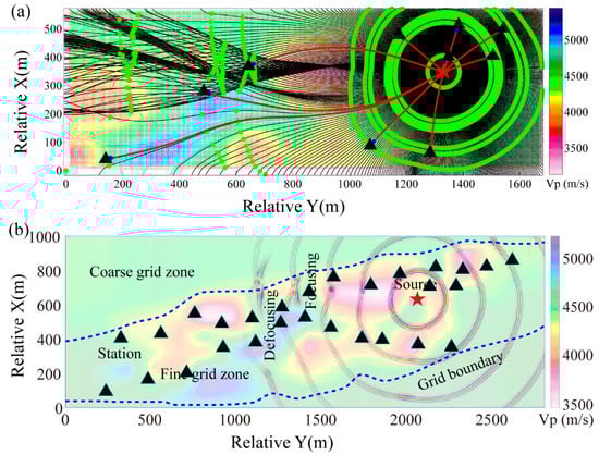
Figure 4.
Ray propagation paths of the shooting method and schematic diagram of wavefield propagation by the spectral element method (SEM) modeling. (a) Ray propagation paths of the shooting method (modified from Wang et al. [6]). The background is a 2D sliced plane of the 3D velocity model, which is determined through the least square vertical distance from all sensors to the plane. The black triangles represent the sensor locations, and the red star denotes the source location. The black thin curves are ray propagation paths from different angles of the source, the red lines are ray propagation paths from the source to each sensor, and the green curves are the wavefronts; (b) Schematic diagram of wavefield propagation by SEM modeling. The time interval between adjacent wavefronts is 0.004 s, and the wavefield amplitude is globally normalized to show the attenuation, focusing, and defocusing characteristics of wavefield propagation in complex media. The dotted line shows the boundary of the fine grid region.
4.2. Case of Waveform Modeling and Source-Time Function Estimating
Taking the black star in Figure 4 as the source location and setting the source as an explosion source, and considering that the main frequency of a blasting event is usually within 250 Hz and the dominant frequency is usually within 120 Hz, a Ricker wavelet with dominant frequency 120 Hz is taken as the source-time function for SEM modeling. The time interval between adjacent wavefronts shown in Figure 4 is 0.004 s. It can be seen that the SEM method can precisely model the focusing and defocusing effects in complicated velocity regions compared with the ray tracing technique (Figure 1 in [6]): The low-velocity regions have focusing effects on the transmitted waves and produce diffraction and multi-path effects. There are defocusing effects on waves propagating through the high-velocity regions, which are usually difficult to rapidly and appropriately calculate travel-time field of waves passing through the strong high-velocity regions by using the ray-shooting method. In addition, the wavefield attenuates rapidly with the increase of propagation distance, indicating that the SEM modeling can correctly consider the variation of waveform amplitude so as to make full use of information contained in the observed waveforms.
To test location performance, eight blasting events with pre-measured locations were selected for application test, and the event location information is listed in Table 1 of [6]. The blasting event two was taken as the example to illustrate the source-time function estimation performance when using the DD-SVD-FD wavelet. After estimating the source-time function by the DD-SVD-FD wavelet and fractional-order Gaussian function, the corresponding modeled waveforms are shown as red and blue curves in Figure 5a, respectively. When estimating source-time function with the fractional-order Gaussian function, the optimal fractional-order and dominant frequency are obtained by a grid search procedure for maximum cross-correlation coefficient between data waveform and modeled waveform (Equation (7)). Source-time function estimation using the DD-SVD-FD wavelet is achieved by grid search of fractional order and time scaling factor a. The normalized amplitude spectra corresponding to the colored waveforms are shown in Figure 5b, in which the vertical dotted line indicates the peak frequency, and the shaded region represents the half-bandwidth frequency distribution range. Moreover, the intersection point between the right side of shaded range and curve of amplitude spectrum corresponds to the highest cut-off frequency wh used for wavefield modeling and GSWI location. It can be seen that both synthetic waveforms obtained by the DD-SVD-FD source-time wavelet and fractional-order Gaussian source-time function can reasonably fit the observed waveforms. After carefully comparing the two results, the synthetic waveforms obtained by the DD-SVD-FD wavelet obtain a better fitting degree to the observed waveforms in the time domain and frequency domain through the normalized cross-correlation coefficient improvement. Generally, some small cycle skipping phenomena may occur in the synthetic waveform simulation with inaccurate source-time function for certain frequency bands, which in turn affected the location results. Therefore, a more precise source-time function estimation leads to a better matching between synthetic waveforms and observation waveforms, which can be used to more effectively constrain the source location and is beneficial to the study of microseismic activity.
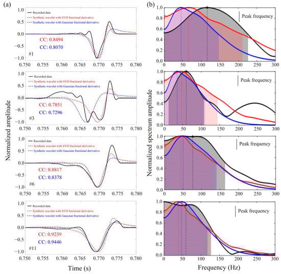
Figure 5.
Fitting performance of windowed observed waveforms and synthetic waveforms based on different source-time function estimation approaches and their corresponding amplitude spectra. (a) Waveform fitting illustration of synthetic waveforms generated by the data-driven singular value decomposition averaged fractional derivative (DD-SVD-FD) source-time wavelet (red curve) and frictional-order Gaussian source-time function (blue curve). The black curve represents the windowed observed waveforms. The normalized cross-correlation coefficient between DD-SVD-FD source-time function and windowed observed waveform is shown in red text, while the normalized cross-correlation coefficient between frictional-order Gaussian source-time function and windowed observed waveform is shown in blue text. The number corresponds to the renumbering of sensors, which is ranked from early to late according to the initial P phase arrival time. (b) Normalized amplitude spectra correspond to the colored waveforms shown in (a). The vertical dotted line is the peak frequency and the shaded region shows the half-bandwidth frequency range.
4.3. MS Location Examples
Taking the blasting events 1 and 3 as the cases to illustrate 3D MS-GSWI location method, their location results are shown in Figure 6 and Figure 7, respectively. Figure 6b–d and Figure 7b–d also demonstrate that velocity parameter sensitivity kernels of cross-correlation travel time anomaly have broader and more reasonable illumination range compared with the simple infinite-frequency assumption-based geometric ray tracing methods (Figure 6b and Figure 7b). The sensitivity kernels of cross-correlation travel time anomaly are closely related to the frequency content of the wavefield, and here only the distribution of sensitivity kernels calculated by the Gaussian source-time function with main frequency of 120 Hz is displayed. If the frequency bands tend to infinite high frequency, the sensitivity kernels of travel time anomaly will shrink to a very narrow tube just like the geometric ray. The sensitivity kernels of travel time based on numerical waveform modeling can better reveal multi-path effects around strong low-velocity anomalies (Figure 6c,d and Figure 7c) and evident wavefield interference influence (Figure 7d). In strongly heterogeneous media, the changes of sensitivity kernels of travel time corresponding to the changes of source location will also present very sophisticated characteristics.
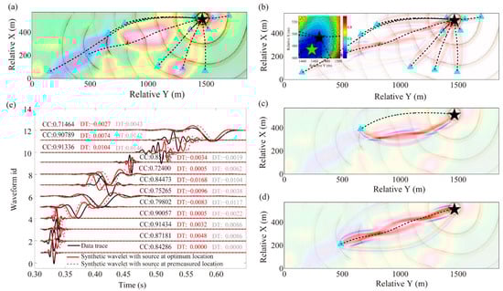
Figure 6.
MS-GSWI location results of the blasting event 1. (a) Ray paths (black dotted curves) from the MS-GSWI location result to corresponding triggered sensors. The background is a 2D sliced plane of the 3D velocity model, the wavefronts modeled by the SEM are shown at a time interval of 0.04 s. It can be observed that each ray is orthogonal to numerical wave front, demonstrating the effectiveness of the SEM modeling. (b) Sensitivity kernels of cross-correlation travel time anomaly from the MS-GSWI location to triggered sensors, which is synthesized by the Gaussian source-time function with a main frequency of 120 Hz. The red to blue color scale shows the intensity value of positive and negative strength of sensitive kernel. The upper left corner shows the misfit contour map of cross-correlation travel time L2 difference between synthetic and observed waveforms. The green and black stars separately indicate the MS-GSWI location and premeasured source location. (c,d) Schematic diagrams of typical sensitivity kernels from the MS-GSWI location to two far away sensors. (e) Fitting performance of SEM modeled waveforms excited from the MS-GSWI location (red curves) and premeasured source location (grey curves) to the observed waveforms (black curves), and red and grey numbers correspond to their cross-correlation travel time difference to observed waveforms. The cross-correlation coefficients between the DD-SVD-FD wavelet modeled waveforms and observed waveforms were displayed as black numbers.
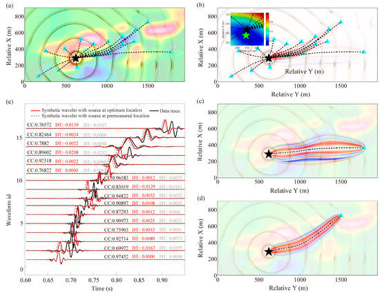
Figure 7.
MS-GSWI location results of the blasting event 3. The rest of the explanation is the same as Figure 6.
The whole velocity field perturbation in the Fresnel zone is weighted by amplitude of sensitivity kernels of travel time anomaly (the red to blue color scale shows the intensity value of positive and negative strength of the sensitive kernel), which finally affects waveforms at sensors and thus leads to complex frequency-dependent perturbation of arrival time and waveform interference. Both the SEM modeled waveforms based on MS-GSWI location result and premeasured true source location can fit the observed waveforms well, with an overall correlation coefficient about 0.8. It should be noted that an appropriate band-pass filtering has been conducted to the waveforms modeled for different sensors to better fit the corresponding observed waveforms. In addition, the total cross-correlation travel time misfit of the modeled waveforms excited from MS-GSWI source location is smaller than that of the premeasured source location, which may be caused by currently inaccurate velocity models. According to misfit distribution of the L2 norm difference of cross-correlation travel time (inserted map in the upper left corner of Figure 6b and Figure 7b), the location determined by the MS-GSWI location is very close to the premeasured source location, and the location errors of blasting events 1 and 3 are 25.0 m and 14.0 m, respectively. The direction-dependent gradient and curvature characteristics of misfit function near MS-GSWI location point could indicate whether the location result along corresponding direction is well constrained.
4.4. MS Location Results
MS-GSWI location results of the eight blasting events are shown in Table 1. The table demonstrates that the maximum location error of the waveform inversion-based location method is 25.0 m and the average error is 15.0 m. There are some uniform velocity model-based location results on the eight blasting events [56,57,58,59], and their average location error is larger than 39.5 m. Particularly, Shang et al. [56] show that location error of the blasting event three in their paper is very large when using automatically picked data. Dong et al. [57] found that the average location error reaches 47.4 m for their selected three events. Li et al. [59] developed a new location method called VFOM to reduce the influence of large picking error, but still obtained an average error larger than 39.5 m. The average error obtained by Wang et al. [6] using 3D ray tracing-based location method is reduced to 26.2 m, which confirms the importance of velocity model accuracy to a mine MS location. Furthermore, Wang et al. [7] utilized a 3D Gaussian beam-based reverse-time migration location method, which has an average location error of only 17.0 m.

Table 1.
Location errors of the eight premeasured blasting events using different location methods.
The research [56,57,58,59] used homogeneous velocity models and straight ray paths to locate an event, while Wang et al. [6] used a 3D ray tracing-based shooting method. For the shooting method, we discretized the 3D space onto a grid with 10 m spacing, then an initial ray set with a 1° interval from the source was adopted for the first time search of ray tracing, which followed Snell’s law between grids, and the two closest rays to the sensor were selected, then we narrowed the ray path region by the bisection method until the distance between the ray path and the sensor was smaller than 0.1 m, which was set as the ray path from the source to the sensor. Furthermore, there are some other ray tracing methods and codes/software packages, such as Lee and Lahr [60] published a 1D velocity model-based location method-HYP071 (software package is available through http://pubs.usgs.gov/of/1999/ofr-99-0023/), and its updated vision that considers different phase arrival time is also available (HYPOSAT, ftp://ftp.norsar.no/pub/outgoing/johannes/hyposat/); Rawlinson and Sambridge [61] developed a multi-stage fast marching method (FMM) for 3D travel time calculation (FMTOMO, http://rses.anu.edu.au/~nick/fmtomo.html), and it can be used for source location and tomography; another widely used ray tracing location method is the double difference approach proposed by Waldhauser and Ellsworth [62] (hypoDD, http://geophysics.eas.gatech.edu/people/cwu/teaching/hypoDD/hypoDD.html#part1_2), they assumed that the propagation paths of wavefields generated by two adjacent seismic events are similar, which effectively reduces the influences of structural anomalies due to the similar ray path from receiver to adjacent earthquakes.
The location results in this study are similar to those obtained by the 3D Gaussian beam-based method, proving that the location method considering finite-frequency effects of wave propagation is significantly superior to the geometric ray tracing-based location. According to Wang et al. [50] and Virieux and Operto [51], the velocity model used in this paper has a resolution of about 50 m. In addition, the Gaussian beam-based method approximately solves the wave equations in a local region around the ray path, thus, partial ray tracing operation is still needed. The modeling accuracy of the Gaussian beam method is lower than that of numerically solving the complete wave equation. If finite-frequency effects are considered by using challenging full waveform inversion, a 3D velocity model with higher resolution could be obtained, which will result in better location results using the proposed MS-GSWI location method.
5. Discussions
5.1. 3D Green’s Function Database Modeling
In waveform inversion, the 3D Green’s function database modeling for a single source point with the finest grid (10 × 10 × 10 m3) is about 120 cpu-hours. Especially when the full-space grid search strategy is adopted, the workload of modeling the Green’s functions from all candidate source grid points to sensors is directly proportional to the total number of spatial grid points. Therefore, this study submitted parallel tasks on local clusters with 2 eight-cores Intel E5-2680 2.7 GHz processors and introduced the reciprocity theorem into wavefield modeling in a mine, which can rapidly compute the Green’s functions using fewer global simulations. The current supercomputing resources can finish the construction of the 3D Green’s function database with fine grid for a whole mining region in two or three days. To further improve the computational efficiency, the workload of waveform inversion and storage requirements of the Green’s function database are reduced by the multi-scale mesh modeling strategy that is similar to Fichtner et al. [63]. The next steps can be realized through a laptop at a quick calculation. If there is more prior knowledge about the regions where MS events occur frequently, the combination of reciprocity theorem and multi-scale grid search could further reduce the wavefield modeling workload and storage requirement of the Green’s function database effectively, which can be generalized for simultaneous multi-source locating in the future.
In addition, under the current limitations of single-component sparse monitoring network and dataset with insufficient signal-to-noise ratio, we have not been able to obtain an appropriate elastic parameter model better than the currently used isotropic Vp tomographic model. Therefore, pure scalar acoustic wave modeling with a rough or simple velocity model is used (corresponding to acoustic pressure field records) to carry out studies in many current exploration-scale microseismic applications. However, the simplified velocity model is not accurate enough in the estimation of the strength of velocity anomalies and geometrical characteristic of the strong structure heterogeneities, such that the next stage task is to further improve the resolution of the structure parameter model. According to the complicated relationship between the spatial resolution of the target model and various control factors, the waveform inversion aiming at the broadband waveform dataset (such as joint tomography or full waveform inversion) can be performed based on accurate wavefield modeling considering that the practical waveform records presents a limited frequency band distribution. High-resolution structure parameter waveform inversion approach considers the wavefield finite frequency effect to improve the model resolution. In the future, when the mining region deploys multi-component monitoring network to obtain waveform data with higher signal-to-noise ratio, a more complete three-component Green’s function database based on the elastic wave equation modeling will be generated for further implementing full centroid inversion based on multi-component waveform data.
5.2. Estimation of the Source-Time Function
In many studies on a MS location and natural seismic source parameter investigation, the second-order Gaussian wavelet (Ricker wavelet) or simple Gaussian function is often used as the source-time function to generate synthetic waveforms. However, the time domain Gaussian or Ricker function is simply distributed in a symmetrical shape with respect to the main peak, and it has limited fitting performance to asymmetric or more complex waveforms. For the fractional-order Gaussian function proposed by Wang [48], better waveform fitting performance is obtained through searching for the best fractional-order derivate u and dominant frequency w0 through normalized cross-correlation coefficients between the modeled waveforms and target data waveforms. However, its application is still focused on the monitoring operation with densely distributed stations and highly similar waveforms. The stations in a mine MS monitoring network are usually sparsely distributed and have large waveform variation with wave propagating distances, which result in more complex and dissimilar waveforms. In this paper, we introduced the fractional-order derivative and time scaling factor into a source-time function estimation procedure based on DD-SVD-FD wavelet. This technique fully considers variability and complexity of target-observed waveforms and can better fit the recording waveforms in a mine. The waveform-based grid search location method proposed here is a kind of source scanning algorithm by performing grid search strategy to evaluate the matching between the recording and synthetic waveforms, and the misfit minimization corresponding event location. Such that, an improved source-time function estimation and corresponding forward modeling is important for precisely computing misfit function value for each candidate source grid.
6. Conclusions
This study proposed a 3D multi-scale grid search and waveform inversion-based location method (GSWI location) into mine MS location, and the main conclusions are made as follows: (1) The combination of reciprocity theorem and multi-scale grid generation and search strategy effectively reduces modeling computational cost and storage requirement of the 3D Green’s function database. The establishment of the Green’s function database is favorable to the multi-scale grid search, which is helpful to find the globally optimal source location that fits the observed waveforms best. (2) The SEM method can effectively realize precise waveform modeling in complex structures, and the frequency-dependent sensitivity kernels of travel time anomaly have more accurate spatial distribution and intensity characteristics than the ray tracing methods. (3) Both the proposed DD-SVD-FD wavelet and fractional-order Gaussian function can well estimate the source-time function to generate synthetic waveforms fitting the recording waveforms. The synthetic waveforms obtained by the DD-SVD-FD source wavelet taking advantage of recording waveforms have better fitting performance, and have better data adaptability and versatility. (4) The average location error of the 3D GSWI for eight blasting events is only 15.0 m, which is smaller than that of the 3D ray tracing location method (26.2 m) with the same 3D velocity model. This proves that the waveform inversion-based location method can better constrain source location in complex regions than the simplified ray tracing method only based on arrival time pickings. In the future, taking advantage of resolution improved 3D velocity model through full waveform inversion approach relying on numerical wave-equation-solver can further raise location accuracy.
Author Contributions
Methodology, Y.W.; software, Y.W.; resources, X.S.; writing—original draft preparation, X.S.; writing—review and editing, Z.W. and R.G. All authors have read and agreed to the published version of the manuscript.
Funding
This research was funded by the National Natural Science Foundation of China (NSFC) under Grant 52004041 and Grant 41804045, the China Postdoctoral Science Foundation under Grant 2020T130757, the Basic Scientific Research Operating Expenses of Central Universities under Grant 2020CDJQY-A047, and Chognqing Postdoctoral Science Foundation under Grant cstc2020jcyj-bshX0106.
Conflicts of Interest
The authors declare no conflict of interest.
References
- Feng, G.L.; Feng, X.-T.; Chen, B.R.; Xiao, Y.X.; Jiang, Q. Sectional velocity model for microseismic source location in tunnels. Tunn. Undergr. Space Technol. 2015, 45, 73–83. [Google Scholar] [CrossRef]
- Shang, X.; Tkalčić, H. Point-source inversion of small and moderate earthquakes from P-wave polarities and P/S amplitude ratios within a hierarchical Bayesian framework: Implications for the Geysers earthquakes. J. Geophys. Res.-Sol. Ea. 2020, 125, e2019JB018492. [Google Scholar] [CrossRef]
- Feng, G.L.; Feng, X.T.; Chen, B.R.; Xiao, Y.X.; Liu, G.F.; Zhang, W.; Hu, L. Characteristics of microseismicity during breakthrough in deep tunnels: Case study of Jinping-II hydropower station in China. Int. J. Geomech. 2020, 20, 04019163. [Google Scholar] [CrossRef]
- Dong, L.J.; Zou, W.; Sun, D.Y.; Tong, X.J.; Li, X.B.; Shu, W.W. Some developments and new insights for microseismic/acoustic emission source localization. Shock Vib. 2019, 2019, 1–15. [Google Scholar] [CrossRef]
- Karasözen, E.; Karasözen, B. Earthquake location methods. Int. J. Geomath. 2020, 11. [Google Scholar] [CrossRef]
- Wang, Y.; Shang, X.; Peng, K. Relocating mining microseismic earthquakes in a 3-D velocity model using a windowed cross-correlation technique. IEEE Access 2020, 8, 37866–37878. [Google Scholar] [CrossRef]
- Wang, Y.; Shang, X.; Peng, K. Locating mine microseismic events in a 3D velocity model through the Gaussian beam reverse-time migration technique. Sensors 2020, 20, 2676. [Google Scholar] [CrossRef]
- Kim, Y.; Liu, Q.; Tromp, J. Adjoint centroid-moment tensor inversions: Adjoint centroid-moment tensor inversions. Geophys. J. Int. 2011, 186, 264–278. [Google Scholar] [CrossRef]
- Witten, B.; Shragge, J. Image-domain velocity inversion and event location for microseismic monitoring. Geophysics 2017, 82, KS71–KS83. [Google Scholar] [CrossRef]
- Witten, B.; Shragge, J. Microseismic image-domain velocity inversion: Marcellus Shale case study. Geophysics 2017, 82, KS99–KS112. [Google Scholar] [CrossRef]
- Li, L.; Tan, J.; Schwarz, B.; Staněk, F.; Poiata, N.; Shi, P.; Diekmann, L.; Eisner, L.; Gajewski, D. Recent advances and challenges of waveform-based seismic location methods at multiple scales. Rev. Geophys. 2020, 58, e2019RG000667. [Google Scholar] [CrossRef]
- Tkalčić, H.; Dreger, D.S.; Foulger, G.R.; Julian, B.R. The puzzle of the Bardarbunga, Iceland earthquake: No volumetric component in the source mechanism. Bull. Seismol. Soc. Am. 2009, 99, 3077–3085. [Google Scholar] [CrossRef]
- Hsu, Y.J.; Simons, M.; Williams, C. Three-dimensional FEM derived elastic Green’s functions for the coseismic deformation of the 2005 Mw 8.7 Nias-Simeulue, Sumatra earthquake. Geochem. Geophys. Geosystems 2011, 12, Q07013. [Google Scholar] [CrossRef]
- Zeng, H.R.; Song, H.Z. Inversion of source mechanism of 1989 Loma Prieta earthquake by three-dimensional FEM Green’s function. Acta Seismol. Sin. 1999, 12, 249–256. [Google Scholar] [CrossRef]
- Eisner, L.; Clayton, R.W. Simulating strong ground motion from complex sources by reciprocal Green functions. Stud. Geophys. Geod. 2005, 49, 323–342. [Google Scholar] [CrossRef][Green Version]
- Bignardi, S.; Fedele, F.; Yezzi, A. Geometric seismic-wave inversion by the boundary element method geometric seismic. Bull. Seismol. Soc. Am. 2012, 102, 802–811. [Google Scholar] [CrossRef]
- Zhao, Z.; Zhao, Z.; Xu, J.; Kubota, R. Synthetic seismograms of ground motion near earthquake fault using simulated Green’s function method. Chin. Sci. Bull. 2006, 51, 3018–3025. [Google Scholar] [CrossRef]
- Semblat, J.F. Modeling seismic wave propagation and amplification in 1D/2D/3D linear and nonlinear unbounded media. Int. J. Geomech. 2011, 11, 440–448. [Google Scholar] [CrossRef]
- Komatitsch, D.; Vilotte, J.P. The spectral element method: An efficient tool to simulate the seismic response of 2D and 3D geological structures. Bull. Seismol. Soc. Am. 1998, 88, 368–392. [Google Scholar]
- Komatitsch, D.; Ritsema, J.; Tromp, J. The spectral-element method, Beowulf computing, and global seismology. Science 2002, 298, 1737–1742. [Google Scholar] [CrossRef]
- Fichtner, A.; Kennett, B.L.N.; Igel, H. Synthetic background for continental-and global-scale full-waveform inversion in the time-frequency domain. Geophys. J. Int. 2008, 175, 665–685. [Google Scholar] [CrossRef]
- Tape, C.; Liu, Q.; Maggi, A. Adjoint tomography of the southern California crust. Science 2009, 325, 988–992. [Google Scholar] [CrossRef]
- Liu, Q.; Polet, J.; Komatitsch, D. Spectral-element moment tensor inversions for earthquakes in Southern California. Bull. Seismol. Soc. Am. 2004, 94, 1748–1761. [Google Scholar] [CrossRef]
- Hejrani, B.; Tkalčić, H.; Fichtner, A. Centroid moment tensor catalogue using a 3-D continental scale Earth model: Application to earthquakes in Papua New Guinea and the Solomon Islands. J. Geophys. Res. Solid Earth 2017, 122, 5517–5543. [Google Scholar] [CrossRef]
- Hejrani, B.; Tkalčić, H. The 20 May 2016 Petermann ranges earthquake: Centroid location, magnitude and focal mechanism from full waveform modelling. Aust. J. Earth Sci. 2019, 66, 37–45. [Google Scholar] [CrossRef]
- McMechan, G.A. Determination of source parameters by wavefield extrapolation. Geophys. J. Int. 1982, 71, 613–628. [Google Scholar] [CrossRef]
- Wu, Y.; McMechan, G.A. Elastic full-waveform inversion for earthquake source parameters. Geophys. J. Int. 1996, 127, 61–74. [Google Scholar] [CrossRef]
- Sen, A.T.; Cesca, S.; Bischoff, M.; Meier, T.; Dahm, T. Automated full moment tensor inversion of coal mining-induced seismicity. Geophys. J. Int. 2013, 195, 1267–1281. [Google Scholar] [CrossRef]
- Ma, J.; Dong, L.; Zhao, G.; Li, X. Focal Mechanism of mining-induced seismicity in fault zones: A case study of Yongshaba mine in China. Rock Mech. Rock Eng. 2019, 52, 3341–3352. [Google Scholar] [CrossRef]
- Cesca, S.; Grigoli, F.; Heimann, S.; Gonzalez, A.; Buforn, E.; Maghsoudi, S.; Blanch, E.; Dahm, T. The 2013 September-October seismic sequence offshore Spain: A case of seismicity triggered by gas injection? Geophys. J. Int. 2014, 198, 941–953. [Google Scholar] [CrossRef]
- Jarillo Michel, O.; Tsvankin, I. Waveform inversion for microseismic velocity analysis and event location in VTI media. Geophysics 2017, 82, WA95–WA103. [Google Scholar] [CrossRef]
- Michel, O.J.; Tsvankin, I. 3D waveform inversion of downhole microseismic data for transversely isotropic media. Geophys. Prospect. 2019, 67, 2332–2342. [Google Scholar] [CrossRef]
- Igonin, N.; Innanen, K. Analysis of simultaneous velocity and source parameter updates in microseismic FWI. In SEG Technical Program Expanded Abstracts; Society of Exploration Geophysicists: Tulsa, OK, USA, 2018. [Google Scholar]
- Wang, H.; Alkhalifah, T. Microseismic imaging using a source function independent full waveform inversion method. Geophys. J. Int. 2018, 214, 46–57. [Google Scholar] [CrossRef]
- Rodriguez, I.V.; Sacchi, M.; Gu, Y.J. Simultaneous recovery of origin time, hypocentre location and seismic moment tensor using sparse representation theory. Geophys. J. Int. 2012, 188, 1188–1202. [Google Scholar] [CrossRef]
- Shekar, B.; Sethi, H.S. Full-waveform inversion for microseismic events using sparsity constraints. Geophysics 2018, 84, KS1–KS12. [Google Scholar] [CrossRef]
- Tong, P.; Yang, D.; Liu, Q.; Yang, X.; Harris, J. Acoustic wave-equation-based earthquake location. Geophys. J. Int. 2016, 205, 464–478. [Google Scholar] [CrossRef]
- Huang, C.; Dong, L.; Liu, Y.; Yang, J. Acoustic wave-equation based full-waveform microseismic source location using improved scattering-integral approach. Geophys. J. Int. 2017, 209, 1476–1488. [Google Scholar] [CrossRef]
- Huang, C.; Dong, L.G.; Liu, Y.Z.; Yang, J.Z. Waveform-based source location method using a source parameter isolation strategy. Geophysics 2017, 82, KS85–KS97. [Google Scholar] [CrossRef]
- Tarantola, A. Inversion of seismic reflection data in the acoustic approximation. Geophysics 1984, 49, 1259–1266. [Google Scholar] [CrossRef]
- Bouchon, M. Teleseismic body wave radiation from a seismic source in a layered medium. Geophys. J. Int. 1976, 47, 515–530. [Google Scholar] [CrossRef]
- Graves, R.; Wald, D. Resolution analysis of finite fault source inversion using 1D and 3D Green’s functions: 1. Strong motions. J. Geophys. Res. 2001, 106, 8745–8766. [Google Scholar] [CrossRef]
- Eisner, L.; Clayton, W. A reciprocity method for multiple-source simulations. Bull. Seismol. Soc. Am. 2001, 91, 553–560. [Google Scholar] [CrossRef]
- Eisner, L.; Clayton, R.W. A Full waveform test of the Southern California velocity model by the reciprocity method. Pure Appl. Geophys. 2002, 159, 1691–1706. [Google Scholar] [CrossRef][Green Version]
- Lee, E.J.; Chen, P.; Jordan, T.H.; Wang, L. Rapid full-wave centroid moment tensor (CMT) inversion in a three-dimensional earth structure model for earthquakes in Southern California. Geophys. J. Int. 2011, 186, 311–330. [Google Scholar] [CrossRef]
- Zhu, L.; Zhou, X. Seismic moment tensor inversion using 3D velocity model and its application to the 2013 Lushan earthquake sequence. Phys. Chem. Earth Parts A B C 2016, 95, 10–18. [Google Scholar] [CrossRef]
- Seriani, G.; Priolo, E. Spectral element method for acoustic wave simulation in heterogeneous media. Finite Elem. Anal. Des. 1994, 16, 337–348. [Google Scholar] [CrossRef]
- Wang, Y. Frequencies of the Ricker wavelet. Geophysics 2015, 80, A31–A37. [Google Scholar] [CrossRef]
- Freire, S.; Ulrych, T. Application of singular value decomposition to vertical seismic profiling. Geophysics 1988, 53, 778–785. [Google Scholar] [CrossRef]
- Wang, Z.; Li, X.; Zhao, D.; Shang, X.; Dong, L. Time-lapse seismic tomography of an underground mining zone. Int. J. Rock Mech. Mini. 2018, 107, 136–149. [Google Scholar] [CrossRef]
- Virieux, J.; Operto, S. An overview of full-waveform inversion in exploration geophysics. Geophysics 2009, 74, WCC1–WCC26. [Google Scholar] [CrossRef]
- Li, X.; Shang, X.; Wang, Z.; Dong, L.; Weng, L. Identifying P-phase arrivals with noise: An improved Kurtosis method based on DWT and STA/LTA. J. Appl. Geophys. 2016, 133, 50–61. [Google Scholar] [CrossRef]
- Shang, X.; Li, X.; Morales-Esteban, A.; Chen, G. Improving microseismic event and quarry blast classification using artificial neural networks based on principal component analysis. Soil Dyn. Earthq. Eng. 2017, 99, 142–149. [Google Scholar] [CrossRef]
- Wu, Q.; Li, X.; Weng, L.; Li, Q.; Zhu, Y.; Luo, R. Experimental investigation of the dynamic response of prestressed rockbolt by using an SHPB-based rockbolt test system. Tunn. Undergr. Space Technol. 2019, 93, 103088. [Google Scholar] [CrossRef]
- Si, X.; Gong, F. Strength-weakening effect and shear-tension failure mode transformation mechanism of rockburst for fine-grained granite under triaxial unloading compression. Int. J. Rock Mech. Min. Sci. 2020, 131, 104347. [Google Scholar] [CrossRef]
- Shang, X.; Li, X.; Morales-Esteban, A.; Dong, L. Enhancing micro-seismic P-phase arrival picking: EMD-cosine function-based denoising with an application to the AIC picker. J. Appl. Geophys. 2018, 150, 325–337. [Google Scholar] [CrossRef]
- Dong, L.; Shu, W.; Li, X.; Han, G.; Zou, W. Three dimensional comprehensive analytical solutions for locating sources of sensor networks in unknown velocity mining system. IEEE Access 2017, 5, 11337–11351. [Google Scholar] [CrossRef]
- Dong, L.; Zou, W.; Li, X.; Shu, W.; Wang, Z. Collaborative localization method using analytical and iterative solutions for microseismic/acoustic emission sources in the rockmass structure for underground mining. Eng. Fract. Mech. 2019, 210, 95–112. [Google Scholar] [CrossRef]
- Li, X.B.; Wang, Z.W.; Dong, L.J. Locating single-point sources from arrival times containing large picking errors (LPEs): The virtual field optimization method (VFOM). Sci. Rep. 2016, 6, 19205. [Google Scholar] [CrossRef]
- Lee, W.; Lahr, J. A computer program for determining local earthquake hypocenter, magnitude, and first motion pattern of local earthquakes. US Geol. Surv. Rep. 1975, 75, 1–116. [Google Scholar]
- Rawlinson, N.; Sambridge, M. Wave front evolution in strongly heterogeneous layered media using the fast marching method. Geophys. J. Int. 2004, 156, 631–647. [Google Scholar] [CrossRef]
- Waldhauser, F.; Ellsworth, W.L. A Double-difference earthquake location algorithm: Method and application to the Northern Hayward Fault, California. Bull. Seismol. Soc. Am. 2000, 90, 1353–1368. [Google Scholar] [CrossRef]
- Fichtner, A.; Trampert, J.; Cupillard, P.; Saygin, E.; Taymaz, T.; Capdeville, Y.; Villaseñor, A. Multiscale full waveform inversion. Geophys. J. Int. 2013, 194, 534–556. [Google Scholar] [CrossRef]
Publisher’s Note: MDPI stays neutral with regard to jurisdictional claims in published maps and institutional affiliations. |
© 2020 by the authors. Licensee MDPI, Basel, Switzerland. This article is an open access article distributed under the terms and conditions of the Creative Commons Attribution (CC BY) license (http://creativecommons.org/licenses/by/4.0/).