Language Model Using Neural Turing Machine Based on Localized Content-Based Addressing

Abstract

The performance of a long short-term memory (LSTM) recurrent neural network (RNN)-based language model has been improved on language model benchmarks. Although a recurrent layer has been widely used, previous studies showed that an LSTM RNN-based language model (LM) cannot overcome the limitation of the context length. To train LMs on longer sequences, attention mechanism-based models have recently been used. In this paper, we propose a LM using a neural Turing machine (NTM) architecture based on localized content-based addressing (LCA). The NTM architecture is one of the attention-based model. However, the NTM encounters a problem with content-based addressing because all memory addresses need to be accessed for calculating cosine similarities. To address this problem, we propose an LCA method. The LCA method searches for the maximum of all cosine similarities generated from all memory addresses. Next, a specific memory area including the selected memory address is normalized with the softmax function. The LCA method is applied to pre-trained NTM-based LM during the test stage. The proposed architecture is evaluated on Penn Treebank and enwik8 LM tasks. The experimental results indicate that the proposed approach outperforms the previous NTM architecture.

1. Introduction

A language model (LM) estimates the probability of the current word based on the previous word sequence. For the word sequence $W=(w_1,w_2,...,w_N)$, the probability of the LM is denoted as $P(W)$.

$$P(W)=P(w_1,w_2,...,w_N)$$

(1)

where N is the length of W. When the number of words in the word history $(w_1,w_2,...,w_{i-1})$ increases, it becomes increasingly difficult to calculate the probability for the current word $w_i$, because the word history will not appear in the text corpus. For this reason, the Markov assumption is applied to the LM to compute $P(w_i|w_1,...,w_{i-1})$. Here, the length of the word sequence which affects $w_i$ is $(n-1)$.

For modeling the LM, the conventional method is an n-gram but it has the following two problems: an unseen word sequence problem and a limitation in the length of the word history. To address these problems, an LM using a deep neural network (DNN) was proposed to model word sequences [1]. It could predict the probability of the unseen word sequence with a high-dimensional hyperplane of the DNN. However, the DNN-based LM cannot solve the limitation in the length of the word history.

To solve the aforementioned limitation, a recurrent neural network (RNN) was used to model the longer word sequence [2]. In the RNN-based LM, a recurrent hidden layer performs the role of memory through recurrence. The recurrent hidden layer can learn from the first word to the $(n-1)$-th word. Therefore, the RNN-based LM solves the aforementioned issue. However, the output of the recurrent hidden layer trained in the previous time step is gradually vanished and is replaced by the current input when the time step is increased. This is referred to as the vanish gradient problem.

For the vanish gradient problem of the RNN-based LM, a long short-term memory (LSTM) [3] was used in the RNN-based LM [4]. The LSTM consists of an input gate, output gate, forget gate, and one or more memory cells [3]. The LSTM RNN-based LM stores the word sequence in the memory cells of the hidden nodes and deletes previous information of the word history depending on the context. However, LSTM language models can effectively use only 200 words or character sequences on average [5]. Therefore, although the LSTM RNN can potentially encode longer contextual information, the LSTN RNN cannot solve the limitation that exists in the length of the word history.

Recently, attention mechanisms have been used in sequence-to-sequence models such as LMs. An advantage of using the attention mechanism is that it supports the interpretation of deep learning models by showing how a deep learning model attends to different blocks of the input sequence [6]. Typical attention-based deep learning models are a Transformer [7] and a neural Turing machine (NTM) architecture [8].

The Transformer replaces LSTM RNN models with multi-head self-attention and positional encoding. Multi-head self-attention computes a sequence of vector-space representations related to different positions in a sequence. Positional encoding makes the Transformer understand long-range dependency with relative word or character positions. The Transformer has been used in LMs, and has been reported to significantly outperform LSTM RNN-based LMs [9]. However, the Transformer can only be treated with a fixed-length input sequence [10]. The input sequence has to be divided into a number of sub-sequences before being input to the Transformer. Transformer-XL [10], GPT-2 [11], and bidirectional encoder representations from Transformers (BERT) [12] are proposed to solve the aforementioned problem of the Transformer.

Another attention-based deep learning model is the NTM architecture. The NTM architecture comprises a controller and an external memory [8]. The controller is based on previous deep learning model topologies. The external memory comprises M-dimensional vectors. The controller writes its output to the external memory and reads information from the external memory. Recently, the performance of NTM architectures has been improved using a memory de-allocation mechanism [13,14]. We refer to this NTM architecture as the memory de-allocation mechanism-based NTM (MDM-NTM) architecture [14]. In [15], an NTM-based LM was first proposed on the Penn Treebank (PTB) dataset [16]. In addition, the NTM-based LM using a highway network-based controller showed performance improvement on the PTB dataset [17].

However, the MDM-NTM architecture presented a problem in content-based addressing for generating attention vectors [18]. Content-based addressing calculates a cosine similarity value between a key generated by the controller and a vector of the external memory [19]. This addressing is necessary to access all memory addresses to calculate the cosine similarity and softmax normalization [20]. This causes the MDM-NTM to infer the wrong answer because the controller obtains information that is not related to the input from the external memory. Hence, content-based addressing is required to read an area of the external memory related to the input.

In this paper, we propose an NTM architecture using localized content-based addressing (LCA-NTM). The LCA method searches a memory address, and cosine similarity of this address is the closest to 1. Next, softmax normalization is performed on a selected area of the external memory. This area includes the d memory addresses on both sides of the selected memory address. The LCA method is applied to test stage on pre-trained NTM-based LM. We evaluated the proposed LCA-NTM-based LM on the PTB LM task and the enwik8 LM task.

2. Related Works

Language modeling has two important problems: (1) unseen word sequence problem and (2) a limitation in the length of the longer word history. To solve the unseen word sequence problem, a DNN was used in the LM [1]. In DNN-based LMs, a semantic embedding vector that expresses semantic information in 8-10 words was used as the input of the DNN for the improvement of a model performance [21]. In addition, an optimization method of calculation in a softmax layer was proposed [22]. However, the DNN-based LM has the limitation of the length of the word history. The limitation occurs because the number of input layers increases as the number of words in context information increases.

RNN was applied to the LM for training with a longer word history [2]. In RNN-based LMs, one word is used as an input, and the output of the recurrent hidden layer at time $(t-1)$ is also used as input. Therefore, recurrent hidden layers maintain information of longer word sequences. Therefore, it solves the problem of the limitation in the length of the longer word history. Discriminant training [23], class-based clustering [24], and noise-contrastive estimation (NCE) [25] were used in the RNN LM for computation speed improvement of the softmax layer, because the dimension of the output layer is the vocabulary size and the number of weight parameters for the RNN-based LM is higher than that of the DNN-based LM. Despite the recurrent hidden layer, the RNN-based LM is difficult to train with a longer word sequence due to gradient vanishing and explosion [26]. The problem is that the error rate converges to zero or infinity when error back-propagation is performed.

To solve the gradient vanishing problem, LSTM was proposed [3]. LSTM is a hidden node structure that consists of one or more memory cells, an input gate, an output gate, and a forget gate. In [27], the performance of LMs based on RNN and LSTM RNN was compared. The LSTM RNN-based LM achieved an absolute improvement of 0.3% in comparison with the RNN-based LM in terms of word error rate (WER) on 12 M words of English Broadcast News transcription task. Although the gradient clipping [28] works well, LSTM has an issue. In addition, the LSTM RNN-based LM cannot treat input sequences longer than 200 words or character sequences [5].

To train LMs on longer word or character sequences, an attention mechanism has been used for LMs. The attention mechanism is an effective method for selecting important information on longer sequences [29]. In the LM, the attention mechanism supports the LM to obtain the ability of how LMs attend to different blocks of input sequences [6]. One of the most widely used attention-based models is the Transformer [7], and it outperforms LSTMs on LM tasks [9]. The Transformer is an encoder-decoder model and relies on a self-attention mechanism [30] on multi-head and positional encoding [7]. Multi-head attention allows the LM to attend to information on different vector-space representations at different positions of a sequence. To provide position information of a sequence to the Transformer, positional encoding is used to obtain long-range dependency from position information on sequence order. However, the Transformer encodes longer context information into a fixed size sequence [10]. In [31], the training dataset was split into shorter chunks and then used as the input of the Transformer. A drawback of this method is that fixed-length chunks lead to the context fragmentation problem [10].

Recently, in order to solve the context fragmentation problem, Transformer-XL [10], GPT-2 [11], and BERT [12] have been proposed and widely used in various tasks. The Transformer-XL uses a hidden state computed at the previous time step as previous context information for the current chunk. This chunk-level recurrence allows the Transformer-XL to maintain long-term dependency and treat the context fragmentation problem. The Transformer-XL showed high performance results of perplexity to 54.52 on the word-level PTB dataset and bits-per-character (BPC) to 0.99 on the character-level enwiki8 dataset [10]. GPT-2 is a multi-layer decoder of the Transformer. In [11], a pre-trained GPT-2 consisted of 12-layer decoder blocks. Each decoder block had 768 hidden nodes and 12 heads for a multi-head self-attention layer. In LM tasks, the GPT-2 achieved a higher performance of BPC to 0.93 with 1542 M weight parameters, in comparison to the result of the Transformer-XL. BERT is a multi-layer bidirectional encoder of the Transformer. BERT is proposed for pre-training deep bi-directional vector space representations by considering left and right context information in all layers. In [12], BERT showed the best performance in NLP tasks, such as a question-answering task and a named entity task.

Another deep learning model based on the attention mechanism is the NTM architecture [8]. The NTM architecture is analogous to the Von Neumann machine with a controller that interacts with an external memory through an attention mechanism. The controller is a deep learning model and the external memory is a set of M-dimensional real-valued vectors. In [8], the experiments showed that the NTM architecture with an LSTM-based controller is capable of learning simple algorithms such as copy, associative recall, and priority sort algorithms. In addition, the MDM-NTM architecture improved the performance of read and write operations from the vanilla NTM architecture [14]. In the MDM-NTM architecture, the memory attention mechanism decides where information is stored in the external memory and maintains the order of sequences through a temporal link. In the experiments, the MDM-NTM architecture showed a performance improvement on the bAbI question-answering task, graph traversal, and block puzzle problems in comparison with the vanilla NTM architecture. Recently, LMs based on the NTM architecture have been proposed. In [15], the NTM architecture was first used for the LM task and it showed perplexity to 98.6 on the word-level PTB dataset. It exhibited better performance than DNN and LSTM-based LMs, but lower performance than the LM based on the Transformer-XL. On the character-level PTB corpus, the MDM-NTM architecture using the highway network-based controller achieved the performance of BPC to 1.147 [17]. It exhibited better performance than the trellis network (BPC 1.158) [32], the AWD-LSTM network (BPC 1.169) [33], and the vanilla Transformer (BPC 1.227) [34].

Despite the success of the LM based on the NTM architecture, content-based addressing of the NTM architecture is necessary to access all external memory addresses to calculate cosine similarity and softmax normalization [20]. To address this issue, content-based addressing is required to select external memory addresses related to the input sequence. In this paper, we propose localized content-based addressing (LCA). We describe more details of the NTM architecture in Section 3 and the proposed LCA-NTM architecture in Section 4.

3. Neural Turing Machine

As shown in Figure 1, the NTM architecture consists of a controller and an external memory [14,18]. The controller is a deep learning model F. The external memory EM is an element of a set ${\mathbb{R}}^{N\times M}$. N is the number of M-dimensional real-valued vectors. If the controller F does not perform a read and write operation to the external memory, then the NTM architecture is equal to the deep learning model topology. We assume that the number of read vectors is R, R read vectors $r_t^i(i=1,2,...,R)$ are generated by the read operation at time t and its dimension is M. The input $x_t$ and R read vectors $r_{t-1}^i$ generated from read operations at time $(t-1)$ are concatenated and then used as the input of F. The controller emits an interface vector ${\xi }_t$ and a controller output vector $o_t$. Moreover, ${\xi }_t$ is used to interact between F and $EM$. After the read operation is performed, R read vectors $r_t^i$ are generated at time t. R read vectors ${r^i}_t$ are used as the input of a deep learning model G. The dimension of an output vector $G(r_t^1,...,r_t^R)$ generated from G is the same as the dimension of $o_t$. Notably, $o_t$ is added to $G(r_t^1,...,r_t^R)$ and then projected into an output vector $y_t$. Furthermore, $y_t$ is equal to the final output of other deep learning model topologies, and the dimension of $y_t$ is the same as the dimension of a target vector.

3.1. Content-Based Addressing and Location-Based Addressing

To generate the read and write weighting vectors, content-based addressing and location-based addressing are performed sequentially in the NTM architecture [14]. The interface vector ${\xi }_t$ is used for addressing these methods. ${\xi }_t$ consists of the following elements: $k_t$, $k{s}_t$, $g_t$, $s_t$, ${\gamma }_t$, $e_t$, and $v_t$. $k_t(\in {\mathbb{R}}^{M\times 1})$ is a key vector at time t. $k{s}_t(\in \mathbb{R})$ is a key strength at time t. $g_t(\in \mathbb{R})$ is an interpolation factor at time t. $s_t(\in {\mathbb{R}}^{3x1})$ is a shift vector at time t. ${\gamma }_t(\in \mathbb{R})$ is a sharpening factor at time t. $e_t(\in {\mathbb{R}}^{M\times 1})$ is an erase vector at time t. $v_t(\in {\mathbb{R}}^{M\times 1})$ is a converted input vector at time t.

For content-based addressing, a cosine similarity is measured with $k_t$ and a vector of each external memory address. The cosine similarity is normalized with the softmax function. The value of content-based addressing in the i-th memory address at time t is determined as follows:

$$C{A}_t\left[i\right]=\frac{exp(CS{(E{M}_t[i,·],k_t)}^{k{s}_t}}{{\sum }_{j=1}^{N}exp(CS{(E{M}_t[j,·],k_t)}^{k{s}_t}}$$

(2)

where $exp$ is an exponential function, $CS$ is the cosine similarity function, and $EM[i,·]$ is the M-dimensional real-valued vector of the i-th external memory address. After content-based addressing, location-based addressing is performed. $C{A}_t$ is interpolated with ${\omega }_{t-1}$ using scalar $g_t$. ${\omega }_{t-1}$ is a weighting vector generated at time $(t-1)$. Interpolated weighting $w_t^{ip}$ is calculated as follows:

$$w_t^{ip}=(1-g_t){\omega }_{t-1}+g_{t}C{A}_t$$

(3)

$w_t^{ip}$ is used to calculate a convolution $w_t^{cv}$ with the shift vector $s_t$. The i-th element of $w_t^{cv}$ is determined as follows:

$$w_t^{cv}\left[i\right]=\sum _{j=0}^{N-1}{w}_t^{ip}\left[j\right]s_t[i-j]$$

(4)

After shifting, sharpening is performed with $w_t^{cv}$ and ${\gamma }_t$ to obtain the final weighting vector ${\omega }_t$. The t-th element of ${\omega }_t$ is calculated as follows:

$${\omega }_t\left[i\right]=\frac{{(w_t^{cv}\left[i\right])}^{{\gamma }_t}}{{\sum }_{j=0}^{N-1}{(w_t^{cv}\left[j\right])}^{{\gamma }_t}}$$

(5)

$k_t$, $k{s}_t$, $g_t$, $s_t$, and ${\gamma }_t$ are assigned to each read and write weighting. In the NTM architecture, the number of read and write weightings is R and one, respectively. Therefore, a dimension of ${\xi }_t$ is $3\times (|k_t|+|k{s}_t|+|g_t|+|s_t|+|{\gamma }_t|)+|e_t|+|v_t|=3\times (M+1+1+3+1)+M+M=5M+18$.

3.2. Read and Write Operations

For the read operation, the NTM architecture attends to a specific external memory area, which is related to the input vector and generates read vectors. The read vector is a M-dimensional real-valued vector, defined as the weighted summation over all vectors of the external memory. Specifically, for the i-th read vector at time t, we define

$$r_t^i=E{M}_t^{\top }{\omega }_t^{r,i}$$

(6)

where $E{M}_t^{\top }$ is a transposed external memory at time t, and ${\omega }_t^{r,i}$ is the i-th N-dimensional read weighting vector at time t. The read weighting vector is an attention vector generated by Section 3.1.

For the write operation, the NTM architecture generates a write weighting vector to determine the external memory addresses and stores the input vector to the selected memory addresses. We define the write operation as follows:

$$E{M}_t=E{M}_{t-1}\circ (OM-{\omega }_t^w{e}_t^{\top })+{\omega }_t^w{v}_t^{\top }$$

(7)

where $E{M}_t$ and $E{M}_{t-1}$ are the external memories at time t and $(t-1)$, respectively. ∘ is the element-wise product. OM is a matrix of the same size as that of the external memory. All elements of OM are 1. $e_t^{\top }$ is a transposed erase vector at time t. The erase vector determines the ratio at which information stored in the external memory is erased. $v_t^{\top }$ is the converted input vector that is transposed at time t. ${\omega }_t^w$ is an N-dimensional write weighting vector at time t. The write weighting vector is the attention vector generated by Section 3.1.

4. Neural Turing Machine Using Localized Content-Based Addressing

Previous content-based addressing, as described in Section 3.1, is necessary for accessing all memory addresses for the calculation of the cosine similarities and using these similarities for generating the attention vector. Consequently, the attention vector can include weights to the memory address, which are not related to the input vector. The unnecessary memory area is reflected in the external memory, which results in performance deterioration.

Hence, we introduce the NTM architecture using LCA-NTM. As shown in Figure 2, cosine similarities are calculated using a key vector $k_t$ and each external memory address. Subsequently, the LCA selects a memory address that shows the maximum cosine similarity. This process is the main difference with vanilla content-based addressing, because vanilla content-based addressing does not select the maximum cosine similarity. If all the cosine similarities are negative, vanilla content-based addressing is used. After searching for the maximum value of cosine similarity, softmax normalization is performed on d memory addresses on both sides of the selected memory address to generate the content-based addressing vector $C{A}_t$. $C{A}_t$[i], where softmax is not performed, is 0. Algorithm 1 describes the proposed LCA procedure in detail.

The proposed NTM architecture attends to a specific memory area selected by LCA. The result of the LCA is the content-based addressing vector. Vanilla location-based addressing is applied to the content-based addressing vector generated from LCA. The final weighting vector is generated by location-based addressing. The proposed LCA method is applied to test the stage on pre-trained NTM-based LM.

For the i-th read vector at time t, we define,

$$r_t^{LCA,i}=E{M}_t^{\top }{\omega }_t^{LC{A}_r,i}$$

(8)

where ${\omega }_t^{LC{A}_r,i}$ is the i-th N-dimensional read weighting vector at time t. The proposed NTM architecture stores the converted input vector to the selected memory addresses. Selected memory addresses are decided by the write weighting vector. We define the write operation in the proposed LCA-NTM architecture as,

$$E{M}_t=E{M}_{t-1}\circ (OM-{\omega }_t^{LC{A}_w}{e}_t^{\top })+{\omega }_t^{LC{A}_w}{v}_t^{\top }$$

(9)

where ${\omega }_t^{LC{A}_w}$ is an N-dimensional write weighting vector at time t. LCA searches for the maximum cosine similarity value. To search for this value, the cosine similarity values are not sorted because all values have to be considered in the deterministic algorithm for obtaining the maximum value. It takes $\mathcal{O}(N)$, where N is the number of vectors in the external memory. The time complexity of softmax normalization used for LCA is $\mathcal{O}(2d+1)$ because the denominator for softmax normalization is dependent on the selected memory area and comprises $(2d+1)$ memory addresses. Therefore, the time complexity of the LCA is $\mathcal{O}(N+2d+1)$.

Algorithm 1: Proposed LCA procedure

5. Experiments and Discussion

To evaluate the proposed LCA-NTM architecture, the vanilla NTM-based LM was trained, and we evaluated the pre-trained NTM-based LM using the LCA method. We trained and tested all LMs on the character-level PTB LM task [16] and the enwik8 LM task [35]. We compared the proposed NTM architecture with state-of-the-art LMs and the MDM-NTM architecture.

5.1. Experimental Environment

The PTB dataset is composed of sentences collected from the Wall Street Journal news domain. The character-level PTB dataset was used in the experiments. However, the character-level PTB dataset does not contain spaces between characters; therefore, it is difficult to recognize a specific word from the character sequence. Hence, space markers (-space-) and a marker for the beginning of a sentence (-bos-) were added to the character-level PTB dataset. Therefore, the total number of characters used for the experiments was 50. The character-level PTB dataset used for the experiments contained 4.88, 0.38, and 0.43 M characters, as the training, validation, and test sets, respectively. The PTB LM task experiment was repeated five times because we verify the stability of hyper-parameters in different LMs and test their generalization.

The enwik8 dataset contains 100 M characters of unprocessed Wikipedia text. The total number of characters was 206. Following previous studies, we split the enwik8 dataset into 90, 5, and 5 M characters for the training, validation, and test sets, respectively. The enwik8 LM task experiment was repeated three times.

We used a 3.40GHz Intel Xeon E5-2643 v4 CPU and four Nvidia GTX 1080 Ti GPUs. We used two evaluation metrics: BPC and training time. BPC is the average number of bits required to encode one character [31]. A bit is used as a unit of entropy. We defined BPC as $loss/log(2)$. To evaluate the inference time of each model, we measured the inference time per batch.

5.2. Experimental Results in Character-Level Penn Treebank LM Task

The LSTM RNN is the baseline LM in the experiments. We trained the baseline LM on PyTorch with the following hyper-parameters: the number of nodes in the embedding layer was 50, the number of hidden layers was 3, the dimension of each hidden layer was 1024, the learning rate was initialized at $1\times {10}^{-1}$, the number of epochs was 300, the number of batches was 6, the weight decay was $1\times {10}^{-6}$, and the length of the back-propagation through time (BPTT) was 120. For training the Transformer-based LM, we used the following hyper-parameters (We used the following open source to train the LSTM RNN and Transformer-based LM: https://github.com/pytorch/examples/blob/master/word_language_model): the number of nodes in the embedding layer was 50, the number of heads in the encoder and decoder was 4, the number of hidden layers was 3, the dimension of each hidden layer was 1024, the learning rate was initialized at $1\times {10}^{-3}$, the number of epochs was 300, the number of batches was 6, the weight decay was $1\times {10}^{-6}$, and the length of the input chunks was 120.

Moreover, we compared the MDM-NTM-based LM with the trellis (https://github.com/locuslab/trellisnet) and AWD-LSTM networks (https://github.com/salesforce/awd-lstm-lm). The hyper-parameters of the trellis and AWD-LSTM networks were the same as those used in previous studies. However, the number of batches was 6 and the BPTT length was 120 for the experiments. In addition, we only applied a dropout factor to the hidden layers, and not the embedding, input, or output layers.

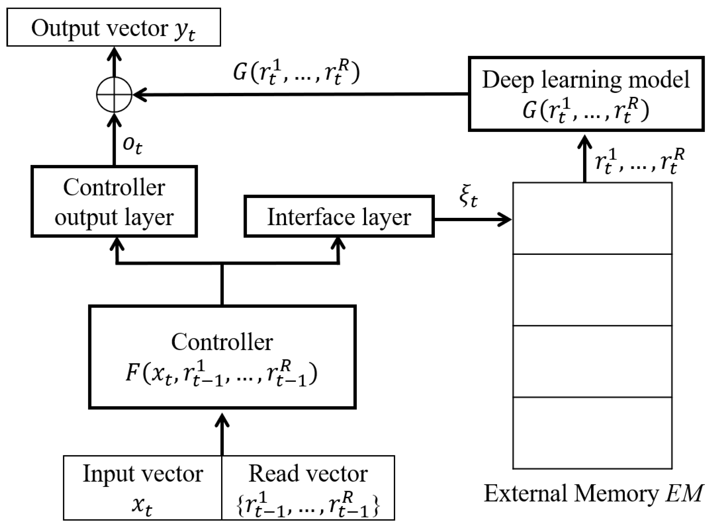
To train the MDM-NTM-based LM, we used the LSTM RNN as the controller. The following hyper-parameters were used for the experiments: the number of nodes in the embedding layer was 50, the number of hidden layers was 3, and the numbers of dimensions of each hidden layer were 1024, 512, and 512. We used the external memory consisting of 1024 vectors. The dimensions of each vector were 512. The learning rate was initialized at $1\times {10}^{-3}$ and reduced on the plateau of an objective function with a factor of $1\times {10}^{-1}$. The number of epochs was 300, the size of the batch was 6, the weight decay was $1\times {10}^{-7}$, and the character sequence length was 120.

Table 1. Evaluation results of MDM-NTM-based LMs on the PTB LM task (nWP, number of weight parameters; nRV, number of read vectors; nVEM, number of vectors in the external memory; WD, weight decay; IT, inference time (ms/batch); $\mu$, mean of BPC results; $\sigma$, standard deviation of BPC results).

						BPC
Model	nWP	nRV	nVEM	WD	IT	Validation		Test
						$\mathbf{\mu }$	$\mathbf{\sigma }$	$\mathbf{\mu }$	$\mathbf{\sigma }$
LSTM	13.2 M	-	-	$1\times {10}^{-6}$	141	1.8949	0.0033	1.8254	0.0031
Transformer	13.2 M	-	-	$1\times {10}^{-6}$	22	1.6042	0.0006	1.5954	0.0004
Trellis Network	13.4 M	-	-	$8\times {10}^{-7}$	4915	1.3858	0.0013	1.3578	0.0019
AWD-LSTM	13.8 M	-	-	$1.2\times {10}^{-6}$	61	1.5224	0.0039	1.4720	0.0036
MDM-NTM	18.3 M	1	65	$1\times {10}^{-7}$	1348	1.7335	0.0011	1.6977	0.0010
	18.3 M	1	129	$1\times {10}^{-7}$	1481	1.6362	0.0008	1.6019	0.0009
	18.3 M	1	257	$1\times {10}^{-7}$	1710	1.6592	0.0011	1.6288	0.0009
	18.3 M	1	513	$1\times {10}^{-7}$	2147	1.6688	0.0006	1.6316	0.0007
	18.3 M	1	769	$1\times {10}^{-7}$	2625	1.6529	0.0006	1.6214	0.0008
	18.3 M	1	1024	$1\times {10}^{-5}$	2872	1.7354	0.0004	1.6998	0.0007
	18.3 M	1	1024	$1\times {10}^{-7}$	2710	1.6330	0.0006	1.5986	0.0007
	23.6 M	2	1024	$1\times {10}^{-5}$	2518	1.7716	0.0003	1.7341	0.0005
	23.6 M	2	1024	$1\times {10}^{-7}$	2590	1.7210	0.0009	1.6906	0.0002
	34.2 M	4	1024	$1\times {10}^{-7}$	3250	1.7428	0.0005	1.7044	0.0009

shows the evaluation results of MDM-NTM-based LMs on the PTB LM task. All MDM-NTM-based LMs had a faster inference time than the trellis network. We measured the performance of the MDM-NTM architecture according to the number of read vectors. The number of read vectors was doubled to evaluate their effect. The MDM-NTM-based LM using a single read vector demonstrated a higher performance with a BPC of 1.5986 than the MDM-NTM-based LMs using two and four read vectors. Each BPC sample of experiment results on the PTB LM task is shown in

Table A1. Each BPC sample of evaluation results on the PTB LM task (nRV, number of read vectors; nVEM, number of vectors in the external memory; nSVEM, number of selected vectors in the external memory; WD, weight decay; DT, data type; TF, Transformer; TL, trellis network; AWD, AWD-LSTM; MDM, MDM-NTM; LCA, LCA-NTM).

Model	nRV	nVEM	nSVEM	WD	DT	Repetition
						1	2	3	4	5
LSTM	-	-	-	$1\times {10}^{-6}$	Val	1.8920	1.8907	1.8954	1.8998	1.8965
					Test	1.8215	1.8299	1.8230	1.8248	1.8278
TF	-	-	-	$1\times {10}^{-6}$	Val	1.6045	1.6039	1.6044	1.6048	1.6032
					Test	1.5957	1.5951	1.5953	1.5961	1.5950
TL	-	-	-	$8\times {10}^{-7}$	Val	1.3848	1.3839	1.3869	1.3873	1.3861
					Test	1.3560	1.3555	1.3589	1.3606	1.3580
AWD	-	-	-	$1.2\times {10}^{-6}$	Val	1.5235	1.5248	1.5160	1.5204	1.5273
					Test	1.4709	1.4750	1.4679	1.4690	1.4772
MDM	1	65	-	$1\times {10}^{-7}$	Val	1.7329	1.7326	1.7354	1.7339	1.7327
					Test	1.6977	1.6965	1.6989	1.6987	1.6967
	1	129	-	$1\times {10}^{-7}$	Val	1.6368	1.6357	1.6374	1.6350	1.6361
					Test	1.6028	1.6012	1.6032	1.6008	1.6015
	1	257	-	$1\times {10}^{-7}$	Val	1.6608	1.6587	1.6574	1.6599	1.6592
					Test	1.6302	1.6281	1.6277	1.6293	1.6287
	1	513	-	$1\times {10}^{-7}$	Val	1.6697	1.6678	1.6685	1.6691	1.6689
					Test	1.6326	1.6309	1.6310	1.6322	1.6313
	1	769	-	$1\times {10}^{-7}$	Val	1.6528	1.6539	1.6530	1.6525	1.6523
					Test	1.6213	1.6227	1.6219	1.6208	1.6203
	1	1024	-	$1\times {10}^{-5}$	Val	1.7351	1.7352	1.7361	1.7355	1.7351
					Test	1.6988	1.6999	1.7009	1.7001	1.6993
	1	1024	-	$1\times {10}^{-7}$	Val	1.6335	1.6332	1.6319	1.6334	1.6330
					Test	1.5995	1.5987	1.5975	1.5992	1.5981
	2	1024	-	$1\times {10}^{-5}$	Val	1.7719	1.7715	1.7714	1.7713	1.7719
					Test	1.7347	1.7342	1.7336	1.7334	1.7346
	2	1024	-	$1\times {10}^{-7}$	Val	1.7197	1.7205	1.7212	1.7225	1.7211
					Test	1.6903	1.6905	1.6907	1.6909	1.6906
	4	1024	-	$1\times {10}^{-7}$	Val	1.7431	1.7425	1.7420	1.7429	1.7435
					Test	1.7052	1.7034	1.7032	1.7047	1.7055
LCA	1	1024	65	$1\times {10}^{-7}$	Val	1.6617	1.6589	1.6569	1.6573	1.6552
					Test	1.6279	1.6267	1.6221	1.6258	1.6220
	1	1024	129	$1\times {10}^{-7}$	Val	1.6479	1.6452	1.6413	1.6415	1.6401
					Test	1.6148	1.6122	1.6081	1.6085	1.6079
	1	1024	257	$1\times {10}^{-7}$	Val	1.6178	1.6171	1.6136	1.6172	1.6203
					Test	1.5669	1.5633	1.5632	1.5635	1.5671
	1	1024	513	$1\times {10}^{-7}$	Val	1.6210	1.6262	1.6213	1.6257	1.6208
					Test	1.6052	1.6100	1.6057	1.6094	1.6051
	1	1024	769	$1\times {10}^{-7}$	Val	1.6403	1.6440	1.6401	1.6420	1.6431
					Test	1.6294	1.6314	1.6273	1.6299	1.6305

.

The analysis for the performance of the MDM-NTM-based LM according to the number of read vectors led to three important findings: (1) the number of weight parameters increased with the number of read vectors. To generate the read vectors, the controller outputs the key vectors. The number of key vectors was the same as the number of read vectors. The key vectors were M-dimensional vectors, where M is a dimension of the vector in the external memory. Furthermore, the number of read vectors affected the dimension of the input layer in the controller, because the read vectors generated at time $(t-1)$ were used as the input to the controller. (2) BPC decreased depending on the number of read vectors. When the MDM-NTM-based LM used one to four read vectors, the performance decreased. This implies that the PTB LM task was insufficient for training all weight parameters of the MDM-NTM-based LM using two or more read vectors. (3) The inference time was disproportional to the number of read vectors. We assumed that a larger number of read vectors required a longer inference time. However, the MDM-NTM-based LM using two read vectors showed a faster inference time than that using one read vector.

We evaluated the performance of the MDM-NTM architecture according to the weight decay. The weight decay reduced the model overfitting by imposing increasingly large penalties as the weight parameters increased [36]. To implement the weight decay, a set of assumed weight parameters such as W, $\frac{1}{2}\lambda W{W}^T$ was added to the loss function and a penalty is imposed. Here, as $\lambda$ increases, an increasingly large penalty was imposed on W. We used two $\lambda$ values, $1\times {10}^{-5}$ and $1\times {10}^{-7}$, during the experiments. Table 1 presents the evaluation results of the MDM-NTM architecture according to weight decay. When we used $\lambda =1\times {10}^{-5}$ for the weight decay, the MDM-NTM-based LM using one and two read vectors demonstrated a BPC of 1.6998 and 1.7341, respectively. The performance of the MDM-NTM-based LM using $\lambda =1\times {10}^{-5}$ for the weight decay was lower than that using $1\times {10}^{-7}$.

Two important findings were observed after analyzing the performance of the MDM-NTM-based LM according to the weight decay: (1) BPC decreased according to the weight decay. When the value of $\lambda$ of the weight decay used in the MDM-NTM-based LM along with a single read vector ranged from $1\times {10}^{-7}$ to $1\times {10}^{-5}$, the performance degraded, that is, BPC increased from 1.5986 to 1.6998. When $\lambda$ of the weight decay was extremely high, the model was trained to underfit. When $\lambda$ of the weight decay was extremely low, the model was trained to overfit. Therefore, the MDM-NTM-based LM using $\lambda =1\times {10}^{-5}$ for the weight decay showed an underfitting in the experiments. (2) The inference time was disproportional to $\lambda$ of the weight decay. We assumed that the training time was the same, even when the MDM-NTM-based LM was trained with any value assigned to $\lambda$ of the weight decay, because the number of weight parameters did not change. However, the experimental results demonstrated that the inference times of each model are different.

We measured the performance of the MDM-NTM architecture according to the number of vectors in the external memory; Table 1 presents the evaluation results. When we used 1024 as the number of vectors in the external memory, the MDM-NTM-based LM demonstrated the highest performance, with a BPC of 1.5986. The inference time decreased when the number of vectors in the external memory decreased.

Three important findings were observed regarding the performance of the MDM-NTM-based LM according to the number of vectors in the external memory: (1) the number of weight parameters is the same, although the number of vectors in the external memory decreased. All MDM-NTM-based LMs used the same controller and all the vectors in the external memory had the same dimensions. The number of weight parameters is related to the controller and the dimension of the vector in the external memory. Therefore, the number of weight parameters is not related to the number of vectors in the external memory. (2) BPC is not proportional to the number of vectors in the external memory. We assumed that the MDM-NTM-based LM demonstrated the highest performance when the number of vectors in the external memory was 120, because the length of the character sequence was limited and the LM could predict the next character without additional vectors in the external memory. However, the MDM-NTM-based LM using the external memory consisting of 129 vectors exhibited a BPC result which was the same as that of the MDM-NTM-based LM using the external memory consisting of 1024 vectors. (3) The inference time is proportional to the number of vectors in the external memory. The time complexity of content-based addressing is $\mathcal{O}(N)$ because of the denominator of the softmax normalization. Therefore, the time spent in the calculation required for softmax normalization influenced the inference time.

We applied the proposed LCA mechanism to the pre-trained MDM-NTM architecture during the evaluation stage. The pre-trained MDM-NTM architecture showed that the highest performance in Table 1 was used. In

Table 2. Evaluation results of LCA-NTM-based LM according to number of selected memory addresses on the PTB LM task (nWP, number of weight parameters; nRV, number of read vectors; nVEM, number of vectors in the external memory; nSVEM, number of selected vectors in the external memory; WD, weight decay; IT, inference time (ms/batch); $\mu$, mean of BPC results; $\sigma$, standard deviation of BPC results).

							BPC
Model	nWP	nRV	nVEM	nSVEM	WD	IT	Validation		Test
							$\mathbf{\mu }$	$\mathbf{\sigma }$	$\mathbf{\mu }$	$\mathbf{\sigma }$
LSTM	13.2 M	-	-	-	$1\times {10}^{-6}$	141	1.8937	0.0032	1.8254	0.0029
Transformer	13.2 M	-	-	-	$1\times {10}^{-6}$	22	1.6042	0.0006	1.5954	0.0004
Trellis	13.4 M	-	-	-	$8\times {10}^{-7}$	4915	1.3858	0.0013	1.3578	0.0019
AWD-LSTM	13.8 M	-	-	-	$1.2\times {10}^{-6}$	61	1.5224	0.0039	1.4720	0.0036
MDM-NTM	18.3 M	1	1024	-	$1\times {10}^{-7}$	2710	1.6330	0.0006	1.5986	0.0007
LCA-NTM	18.3 M	1	1024	65	$1\times {10}^{-7}$	158	1.6580	0.0022	1.6249	0.0024
	18.3 M	1	1024	129	$1\times {10}^{-7}$	154	1.6432	0.0029	1.6103	0.0027
	18.3 M	1	1024	257	$1\times {10}^{-7}$	159	1.6172	0.0021	1.5648	0.0018
	18.3 M	1	1024	513	$1\times {10}^{-7}$	155	1.6230	0.0024	1.6071	0.0022
	18.3 M	1	1024	769	$1\times {10}^{-7}$	157	1.6419	0.0015	1.6297	0.0014

, when the selected memory address was 257, the performance of the LCA-NTM-based LM was 1.5648 BPC. The performance was higher than that of the MDM-NTM-based LM.

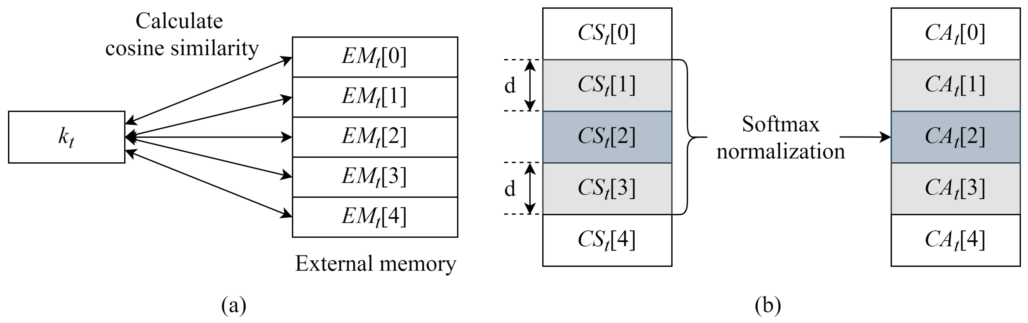
Two important findings were observed regarding the performance of the LCA-NTM-based LM: (1) the BPC of the proposed architecture was lower than that of the MDM-NTM-based LM, except when the selected memory address was 257. We analyzed errors with cosine similarities and discovered that negative values or values close to zero existed, although positive values were also obtained in the cosine similarities of the selected memory address. In the LCA, these cosine similarities were used to generate an attention vector. The proposed NTM architecture yields worse results than the MDM-NTM-based LM. Furthermore, although many of the cosine similarity values were approximately unity, the maximum cosine similarity was always selected in the LCA. If two maximum cosine similarities exist, LCA selects only the first cosine similarity that has the maximum value. These drawbacks led to the performance degradation of the proposed LCA-NTM architecture. (2) The inference time of the proposed NTM architecture in the test stage was twice that of the MDM-NTM-based LM in the test stage. To obtain the maximum cosine similarity, we used the search algorithm for the LCA. The time complexity of the previous content-based addressing was $\mathcal{O}(N)$ because the denominator of softmax normalization had to be computed. However, the time complexity of the LCA was $\mathcal{O}(N+2d+1)$.

5.3. Experimental Results in enwik8 LM Task

We compared the results achieved through the proposed LCA-NTM architecture with those of the Transformer [10]. For the baseline LM, we also used the previous experimental result of the LSTM RNN-based LM [37]. For training the MDM-NTM-based LM, we used the LSTM RNN as the controller. The number of dimensions of the hidden layers was 1024, and the number of hidden layers was 4. We used an external memory consisting of 128 vectors. The number of dimensions of each vector was 256. In addition, the batch size was 20. We could not train or evaluate the large-scale MDM-NTM-based LM because the Nvidia GTX 1080 Ti GPU has a 11-GB memory capacity, and the batch size would have been considerably small if we trained a large-scale MDM-NTM-based LM.

We evaluated the performance of the MDM-NTM architecture according to the number of read vectors.

Table 3. Evaluation results of MDM-NTM-based LMs on the enwik8 LM task (nWP, number of weight parameters; nRV, number of read vectors; nVEM, number of vectors in the external memory; WD, weight decay; IT, inference time (ms/batch); $\mu$, mean of BPC results; $\sigma$, standard deviation of BPC results).

						BPC
Model	nWP	nRV	nVEM	WD	IT	Validation		Test
						$\mathbf{\mu }$	$\mathbf{\sigma }$	$\mathbf{\mu }$	$\mathbf{\sigma }$
LSTM	18.1 M	-	-	-	-	-	-	1.4610	-
Transformer	44.1 M	-	-	-	-	-	-	1.1120	-
MDM-NTM	30.2 M	1	128	$1\times {10}^{-7}$	2940	1.4502	0.0010	1.4475	0.0007
	34.9 M	2	128	$1\times {10}^{-7}$	3118	1.4473	0.0009	1.4419	0.0012
	37.8 M	3	128	$1\times {10}^{-7}$	3397	1.4185	0.0011	1.4117	0.0010
	42.5 M	4	128	$1\times {10}^{-7}$	3644	1.3970	0.0008	1.3922	0.0009

shows the evaluation results. When we used four read vectors, the MDM-NTM-based LM demonstrated the highest BPC performance of 1.3922. The inference time increased when the number of read vectors was increased. Each BPC sample of experiment results on the PTB LM Task is shown in

Table A2. Each BPC sample of evaluation results on the enwik8 LM task (nRV, number of read vectors; nVEM, number of vectors in the external memory; nSVEM, number of selected vectors in the external memory; WD, weight decay; DT, data type; MDM, MDM-NTM; LCA, LCA-NTM).

Model	nRV	nVEM	nSVEM	WD	DT	Repetition
						1	2	3
MDM	1	128	-	$1\times {10}^{-7}$	Val	1.4489	1.4514	1.4503
					Test	1.4468	1.4485	1.4472
	2	128	-	$1\times {10}^{-7}$	Val	1.4461	1.4480	1.4478
					Test	1.4402	1.4429	1.4426
	3	128	-	$1\times {10}^{-7}$	Val	1.4197	1.4188	1.4170
					Test	1.4130	1.4115	1.4106
	4	128	-	$1\times {10}^{-7}$	Val	1.3959	1.3976	1.3975
					Test	1.3915	1.3935	1.3917
LCA	1	128	33	$1\times {10}^{-7}$	Val	1.4095	1.4130	1.4135
					Test	1.4094	1.4103	1.4142
	1	128	65	$1\times {10}^{-7}$	Val	1.4016	1.3979	1.4026
					Test	1.3997	1.3971	1.7017
	1	128	97	$1\times {10}^{-7}$	Val	1.3872	1.3914	1.3899
					Test	1.3867	1.3915	1.3879

.

The analysis of the performance of the MDM-NTM-based LM according to the number of read vectors led to two important findings: (1) BPC decreased depending on the number of read vectors. When the MDM-NTM-based LM used from one to four read vectors, the performance improved. (2) The inference time was proportional to the number of read vectors. We assumed that a larger number of read vectors required a longer inference time. The MDM-NTM-based LM using one read vector showed a faster inference time than that using two or more read vectors.

Furthermore, we applied the proposed LCA mechanism to the pre-trained MDM-NTM architecture during the test stage. The pre-trained MDM-NTM architecture showed that the highest performance in Table 3 was used. In

Table 4. Evaluation results of LCA-NTM-based LM according to number of selected memory addresses on the enwik8 LM task (nWP, number of weight parameters; nRV, number of read vectors; nVEM, number of vectors in the external memory; nSVEM, number of selected vectors in the external memory; WD, weight decay; IT, inference time (ms/batch); $\mu$, mean of BPC results; $\sigma$, standard deviation of BPC results).

							BPC
Model	nWP	nRV	nVEM	nSVEM	WD	IT	Validation		Test
							$\mathbf{\mu }$	$\mathbf{\sigma }$	$\mathbf{\mu }$	$\mathbf{\sigma }$
LSTM	18.1 M	-	-	-	-	-	-	-	1.4610	-
Transformer	44.1 M	-	-	-	-	-	-	-	1.1120	-
MDM-NTM	42.5 M	4	128	-	$1\times {10}^{-7}$	3644	1.3970	0.0008	1.3922	0.0009
LCA-NTM	42.5 M	4	128	33	$1\times {10}^{-7}$	320	1.4120	0.0018	1.4113	0.0021
	42.5 M	4	128	65	$1\times {10}^{-7}$	321	1.4007	0.0020	1.3995	0.0019
	42.5 M	4	128	97	$1\times {10}^{-7}$	318	1.3895	0.0017	1.3887	0.0020

, when the selected memory address was 97, the performance of the LCA-NTM-based LM showed a BPC of 1.3887. The performance was higher than that of the MDM-NTM-based LM. An important finding was observed regarding the performance of the LCA-NTM-based LM. The BPC of the proposed architecture was lower than that of the MDM-NTM-based LM, except when the selected memory address was 97. The performance improvement was not insignificant compared to that observed through the experimental results on the PTB LM task. We analyzed the errors with cosine similarities and discovered that more negative values existed than those in the experimental results on the PTB LM task. Therefore, the proposed NTM architecture applied vanilla content-based addressing, not LCA. These drawbacks led to the performance degradation of the proposed LCA-NTM architecture.

6. Conclusions and Future Work

We presented the LM using the LCA-NTM architecture. The LCA methods selected a memory address that represented the maximum cosine similarity. This differed from vanilla content-based addressing, because vanilla content-based addressing does not search for the maximum cosine similarity. The specific memory area, including the selected memory address, was normalized using a softmax function. For the PTB LM task, when the selected memory address was 257 when applying the LCA, the performance of the LCA-NTM-based LM showed a BPC of 1.5648. For the enwik8 LM task, when the selected memory address was 97, the BPC performance of the LCA-NTM-based LM showed a BPC of 1.3887. These results indicate that the proposed approach outperformed the MDM-NTM-based LM.

In a future work, we intend to modify the LCA-NTM architecture to select multiple addresses according to the cosine similarity. In addition, we will implement methods to improve the inference time of the LCA-NTM architecture. We will also evaluate the LCA-NTM architecture on web-scale LM tasks, such as WikiText-103 and One Billion Word.

References

1. Bengio, Y.; Ducharme, R.; Vincent, P.; Jauvin, C. A neural probabilistic language model. J. Mach. Learn. Res. 2003, 3, 1137–1155. [Google Scholar]
2. Mikolov, T.; Karafiat, M.; Burget, L.; Cernocky, J.; Khudanpur, S. Recurrent neural network based language model. In Proceedings of the 11th Annual Conference of the International Speech Communication Association (INTERSPEEECH), Makuhari, Japan, 26–30 September 2010; pp. 1045–1048. [Google Scholar]
3. Hochreiter, S.; Schmidhuber, J. Long short-term memory. Neural. Comput. 1997, 9, 1735–1780. [Google Scholar] [CrossRef] [PubMed]
4. Emami, A.; Jelinek, F. LSTM neural networks for language modeling. In Proceedings of the 13th Annual Conference of the International Speech Communication Association (INTERSPEECH), Portland, OR, USA, 9–13 September 2012; pp. 1735–1780. [Google Scholar]
5. Khandelwal, U.; He, H.; Qi, P.; Jurafsky, D. Shart nearby, fuzzy far away: How neural language models use context. In Proceedings of the 56th Annual Meeting of the Association for Computational Linguistics (ACL), Melbourne, Australia, 15–20 July 2018; pp. 284–294. [Google Scholar]
6. Belinkov, Y.; Glass, J. Analysis methods in neural language processing: A survey. Trans. Assoc. Comput. Linguist. 2019, 7, 49–72. [Google Scholar] [CrossRef]
7. Vaswani, A.; Shazeer, N.; Parmar, N.; Uszkoreit, J.; Jones, L.; Gomez, A.N.; Kaiser, Ł.; Polosukhin, I. Attention is all you need. Adv. Neural Inf. Process. Syst. 2017, 30, 5998–6008. [Google Scholar]
8. Graves, A.; Wayne, G.; Danihelka, I. Neural Turing machines. arXiv 2014, arXiv:1410.5401. [Google Scholar]
9. Vig, J.; Belinkov, Y. Analyzing the structure of attention in a Transformer language model. In Proceedings of the 2nd BlackboxNLP Workshop on Analyzing and Interpreting Neural Networks for NLP (BlackboxNLP), Florence, Italy, 1 August 2019; pp. 63–76. [Google Scholar]
10. Dai, Z.; Yang, Z.; Yang, Y.; Carbonell, J.; Le, Q.V.; Salakhutdinov, R. Transformer-XL: Attentive language models beyond a fixed-length context. In Proceedings of the 57th Annual Meeting of the Association for Computational Linguistics (ACL), Florence, Italy, 28 July–2 August 2019; pp. 2928–2988. [Google Scholar]
11. Radford, A.; Wu, J.; Child, R.; Luan, D.; Amodei, D.; Sutskever, I. Language models are unsupervised multitask learners. Tech. Rep. 2019, 1–24. [Google Scholar]
12. Devlin, J.; Chang, M.-W.; Lee, K.; Toutanova, K. BERT: Pre-training of deep bidirectional Transformers for language understanding. In Proceedings of the Annual Conference of the North American Chapter of the Association for Computational Linguistics (NAACL-HLT), Minneapolis, MN, USA, 2–7 June 2019; pp. 4171–4186. [Google Scholar]
13. Rae, J.W.; Hunt, J.J.; Harley, T.; Danihelka, I.; Senior, A.; Wayne, G.; Graves, A.; Lillicrap, T.P. Scaling memory-augmented neural networks with sparse reads and writes. In Proceedings of the 30th Conference on Neural Information Processing Systems (NeurIPS), Barcelona, Spain, 5–10 December 2016; pp. 3621–3629. [Google Scholar]
14. Graves, A.; Wayne, G.; Reynolds, M.; Harley, T.; Danihelka, I.; Grabska-Barwińska, A.; Colmenarejo, S.G.; Grefenstette, E.; Ramalho, T.; Agapiou, J.; et al. Hybrid computing using a neural network with dynamic external memory. Nature 2016, 538, 471–476. [Google Scholar] [CrossRef] [PubMed]
15. Ko, W.; Tseng, B.; Lee, H. Recurrent neural network based language modeling with controllable external memory. In Proceedings of the 42nd IEEE International Conference on Acoustics, Speech and Signal Processing (ICASSP), New Orleans, LA, USA, 5–9 March 2017; pp. 5705–5709. [Google Scholar]
16. Marcus, M.; Marcinkiewicz, M.; Santorini, B. Building a large annotated corpus of English: The penn treebank. Comput. Linguist. 1993, 19, 313–330. [Google Scholar]
17. Luo, W.; Yu, F. Recurrent highway networks with grouped auxiliary memory. IEEE Access 2019, 7, 182037–182049. [Google Scholar] [CrossRef]
18. Csordas, R.; Schmidhuber, J. Improving differentiable neural computers through memory masking, de-allocation, and link distribution sharpness control. In Proceedings of the 7th International Conference on Learning Representations (ICLR), New Orleans, LA, USA, 6–9 May 2019; pp. 7299–7310. [Google Scholar]
19. Bai, J.; Dong, T.; Liao, X.; Mu, N. Recurrent neural network with dynamic memory. In Proceedings of the 15th International Symposium on Neural Networks (ISNN), Minsk, Belarus, 25–28 June 2018; pp. 339–345. [Google Scholar]
20. Liu, D.; Chuang, S.; Lee, H. Attention-based memory selection recurrent network for language modeling. arXiv 2016, arXiv:1611.08656. [Google Scholar]
21. Audhkhasi, K.; Sethy, A.; Ramabhadran, B. Semantic word embedding neural network language models for automatic speech recognition. In Proceedings of the 41st IEEE International Conference on Acoustics, Speech and Signal Processing (ICASSP), Shanghai, China, 20–25 March 2016; pp. 5995–5999. [Google Scholar]
22. Huang, Y.; Sethy, A.; Ramabhadran, B. Fast neural network language model lookups at n-gram speeds. In Proceedings of the 18th Annual Conference of the International Speech Communication Association (INTERSPEECH), Stockholm, Sweden, 20–24 August 2017; pp. 274–278. [Google Scholar]
23. Tachioka, Y.; Watanabe, S. Discriminative method for recurrent neural network language models. In Proceedings of the 40th IEEE International Conference on Acoustics, Speech and Signal Processing (ICASSP), South Brisbane, QLD, Australia, 19–24 April 2015; pp. 5386–5390. [Google Scholar]
24. Song, M.; Zhao, Y.; Wang, S. Exploiting different word clusterings for class-based RNN language modeling in speech recognition. In Proceedings of the 42nd IEEE International Conference on Acoustics, Speech and Signal Processing (ICASSP), New Orleans, LA, USA, 5–9 March 2017; pp. 5735–5739. [Google Scholar]
25. Chen, X.; Liu, X.; Gales, M.; Woodland, P. Recurrent neural network language model training with noise contrastive estimation for speech recognition. In Proceedings of the 40th IEEE International Conference on Acoustics, Speech and Signal Processing (ICASSP), South Brisbane, QLD, Australia, 19–24 April 2015; pp. 5411–5415. [Google Scholar]
26. Pascanu, R.; Mikolov, T.; Bengio, Y. On the difficulty of training recurrent neural networks. In Proceedings of the 30th International Conference on Machine Learning (ICML), Atlanta, GA, USA, 16–21 June 2013; pp. 1310–1318. [Google Scholar]
27. Arisoy, E.; Sethy, A.; Ramabhadran, B.; Chen, S. Bidirectional recurrent neural network language models for automatic speech recognition. In Proceedings of the 40th IEEE International Conference on Acoustics, Speech and Signal Processing (ICASSP), South Brisbane, QLD, Australia, 19–24 April 2015; pp. 5421–5425. [Google Scholar]
28. Graves, A. Generating sequences with recurrent neural networks. arXiv 2013, arXiv:1308.0850. [Google Scholar]
29. Xu, K.; Ba, J.L.; Kiros, R.; Cho, K.; Courville, A.; Salakhutdinov, R.; Zemel, R.S.; Bengio, Y. Show, attend and tell: Neural image caption generation with visual attention. In Proceedings of the 32nd International Conference on Machine Learning (ICML), Lile, France, 6–11 July 2015; pp. 2048–2057. [Google Scholar]
30. Lin, Z.; Feng, M.; Santos, C.N.; Yu, M.; Xiang, B.; Zhou, B.; Bengio, Y. A structured self-attentive sentence embedding. arXiv 2017, arXiv:1703.03130. [Google Scholar]
31. Al-Rfou, R.; Choe, D.; Constant, N.; Guo, M.; Jones, L. Character-level language modeling with deeper self-attention. In Proceedings of the 33rd AAAI Conference on Artificial Intelligence (AAAI), Honolulu, HI, USA, 27 January–1 February 2019; pp. 3159–3166. [Google Scholar]
32. Bai, S.; Koiter, J.; Koltun, V. Trellis networks for sequence modeling. In Proceedings of the 7th International Conference on Learning Representations (ICLR), New Orleans, LA, USA, 6–9 May 2019; pp. 1–18. [Google Scholar]
33. Brahma, S. Improved language modeling by decoding the past. In Proceedings of the 57th Annual Meeting of the Association for Computational Linguistics (ACL), Florence, Italy, 28 July–2 August 2019; pp. 1468–1476. [Google Scholar]
34. Fan, A.; Lavril, T.; Grave, E.; Joulin, A.; Sukhbaatar, S. Accessing higher-level representations in sequential Transformers with feedback memory. arXiv 2020, arXiv:2002.09402. [Google Scholar]
35. Mahoney, M. Large Text Compression Benchmark. Available online: http://mattmahoney.net/dc/text.html (accessed on 29 September 2020).
36. Zhang, G.; Wang, C.; Xu, B.; Grosse, R. Three mechanisms of weight decay regularization. In Proceedings of the 7th International Conference on Learning Representations (ICLR), New Orleans, LA, USA, 6–9 May 2019; pp. 1–16. [Google Scholar]
37. Mujika, A.; Meier, F.; Steger, A. Fast-slow recurrent neural networks. In Proceedings of the 31st Conference on Neural Information Processing Systems (NeurIPS), Long Beach, CA, USA, 4–9 December 2017; pp. 5915–5924. [Google Scholar]
Figure 1. Overview of NTM architecture. The controller interacts with the external memory using read and write operations. The external memory stores information, which is a high-dimensional vector of the input vector.
Applsci 10 07181 g001
Figure 2. Overview of localized content-based addressing at time t. (a) The cosine similarity is calculated using a key vector k t and each external memory address. E M t [i] is the i-th vector of the external memory. If we assume that the number of vectors in the external memory is five, we obtain five cosine similarity values C S t . (b) The maximum cosine similarity value is searched. C S t [i] is a cosine similarity value of the i-th memory address. In this Figure, the third memory address shows the maximum cosine similarity value. Subsequently, softmax normalization is performed on specific cosine similarity values calculated from d memory addresses on both sides of the selected memory address. In this Figure, d is 1. After softmax normalization, we obtain a content-based addressing vector C A t . C A t [i] is the i-th value of the content-based addressing vector, whereas w[0] and w[5] are zero. Vanilla location-based addressing is applied to it and then, we obtain the weighting vector.
Applsci 10 07181 g002