Relationship between Aspect Ratio and Crack Density in Porous-Cracked Rocks Using Experimental and Optimization Methods

Abstract

Aspect ratio and crack density are essential parameters to understand the physical properties of porous-cracked rocks, although it is difficult to independently determine each parameter, as both are closely linked. The objective of this study is to propose a relationship between aspect ratio and crack density that can be used to solve for each through experimental and optimization methods. Two different constitutive equations are solved to create expressions explicitly defining aspect ratio and crack density, with all remaining variables arranged as functions of elastic wave velocity. Ten core specimens extracted from construction sites, with diameters of 46 mm, are subjected to artificial weathering to identify how their crack density and aspect ratio evolved with time. The artificial weathering process consisted of chemical and physical weathering cycles using saline solution and slake durability tests, respectively. Compressional and shear wave velocities are measured at every weathering step, and both aspect ratio and crack density are calculated. The random forest as an optimization method is selected to define the important score among input variables. The calculated aspect ratios and crack densities are converted into a crack porosity, the reliability of which is verified through percentage of crack porosity (~6%) in total porosity. This study demonstrates that the relationship between aspect ratio and crack density is robust and has wide-ranging applications in determining individual aspect ratio and crack density parameters in porous-cracked rock.

1. Introduction

Rocks undergo a range of weathering processes driven by changing environmental factors, such as climate, temperature, and precipitation. Characterization of cracks in a rock is one common way to monitor the extent of weathering. Cracks that develop during weathering can reduce the strength and stiffness of a host rock, critically reducing its durability [1,2]. According to Palmstrom [3], cracks have sizes within the range 0.01–1 m, whereas micro-cracks have sizes less than 0.01 m. Visual observation is a common method used to find cracks in rocks, although it is not effective at identifying micro-cracks due to their small size. Given this limitation, crack density, defined as the number of cracks per unit volume of rock, is often used to estimate the number of micro-cracks in a rock instead [4], assuming that their proportions are related. Several researchers have suggested that the crack density can be calculated via the theory of elastic wave propagation [5], which provides a method to estimate the proportions of micro-cracks in the absence of independent constraints.

Biot [6] first established a constitutive equation for wave propagation through a porous medium with a uniform pore pressure by using a stress-strain relationship. Subsequently, Bristow [7] added a crack parameter to this relationship to quantify how crack density affects seismic wave velocity. This theory has since been developed with respect to circular [8] and rectangular [9] cracks, although elastic interactions between cracks must be considered in order for this parameterization to have practical applicability. Budiansky and O’Connell [10] expanded on this work by developing a new model for crack development in rocks, which considered elastic interactions based on self-consistent theory [11]. This parameterization was shown by Berryman [12] to adequately predict interactions between different petrophysical parameters in porous and cracked rocks.

These theories were developed primarily to elastically predict the stress-strain relationship in a porous-cracked rock, rather than quantitatively evaluating the spatial characteristics of the cracks themselves, although some recent models have used this theory to estimate crack densities. Biot [6] showed that elastic moduli and the assumption of elastic behavior are important variables in the wave propagation equation. As such, Adelinet et al. [13] and Tang [14] proposed analytical solutions to investigate changes in crack density due to variations in elastic moduli. Also, since elastic moduli can be inferred from elastic wave velocity, Byun et al. [4] characterized different rock types by estimating their crack density using measured elastic wave velocity data. However, crack density is also a function of aspect ratio, and it is difficult to estimate a reliable crack density without knowing the aspect ratio of the cracks, even if elastic moduli are well constrained. Previous studies of this issue have been limited in their ability to estimate crack densities, as they assumed constant values for aspect ratios. Therefore, in this work, a new relationship is presented that relates crack density and crack aspect ratio, which was parameterized from experimental results. This allows definition of the aspect ratio as a function of the crack density, which allows either of these variables to be determined if the other can be accurately measured.

As the 4th industry technology has developed, data analysis techniques have also been improved, and machine learning (ML) techniques were proposed to reliably define correlations between two or more physical variables or to cluster them [15,16]. The relationship of each different physical quantity is mainly analyzed based on regression analysis, and a deep neural network (DNN) is used to infer nonlinear correlation as part of a supervised learning technique. The method has been widely used in many fields and in particular, it was applied to find excavation type [17], predict permeability [18], digital image of rocks [19] in the field of geotechnical engineering. Furthermore, the random forest (RF) was also used to find the characterization of correlation among input variables as one of the ML algorithms. This method can determine the individual importance of each factor in governing equation by quantitatively providing correlation score. RF constructs a forest composed of multiple trees to restrain overfitting and the technique of bootstrap aggregating for making various data set is used. The random subspace is also applied to expand the number of nodes in decision tree. This algorithm has been applied to find the importance of geometric features in rock surface [20] and input parameter for analyzing stability of landslide [21]. Therefore, this study also tried to find factors that have a major influence on both aspect ratio and crack density by using the ML technique.

In this study, the theoretical background behind elastic moduli, crack density, aspect ratio and random forest is first presented, followed by the results of sensitivity analysis used to understand the characterization of each theory. Next, specimens subjected to artificial weathering experiments for crack generation are described and results for measured elastic wave velocity and calculated elastic moduli are reported. Finally, these data are then used to form a relationship between crack density and aspect ratio.

2. Background Theory

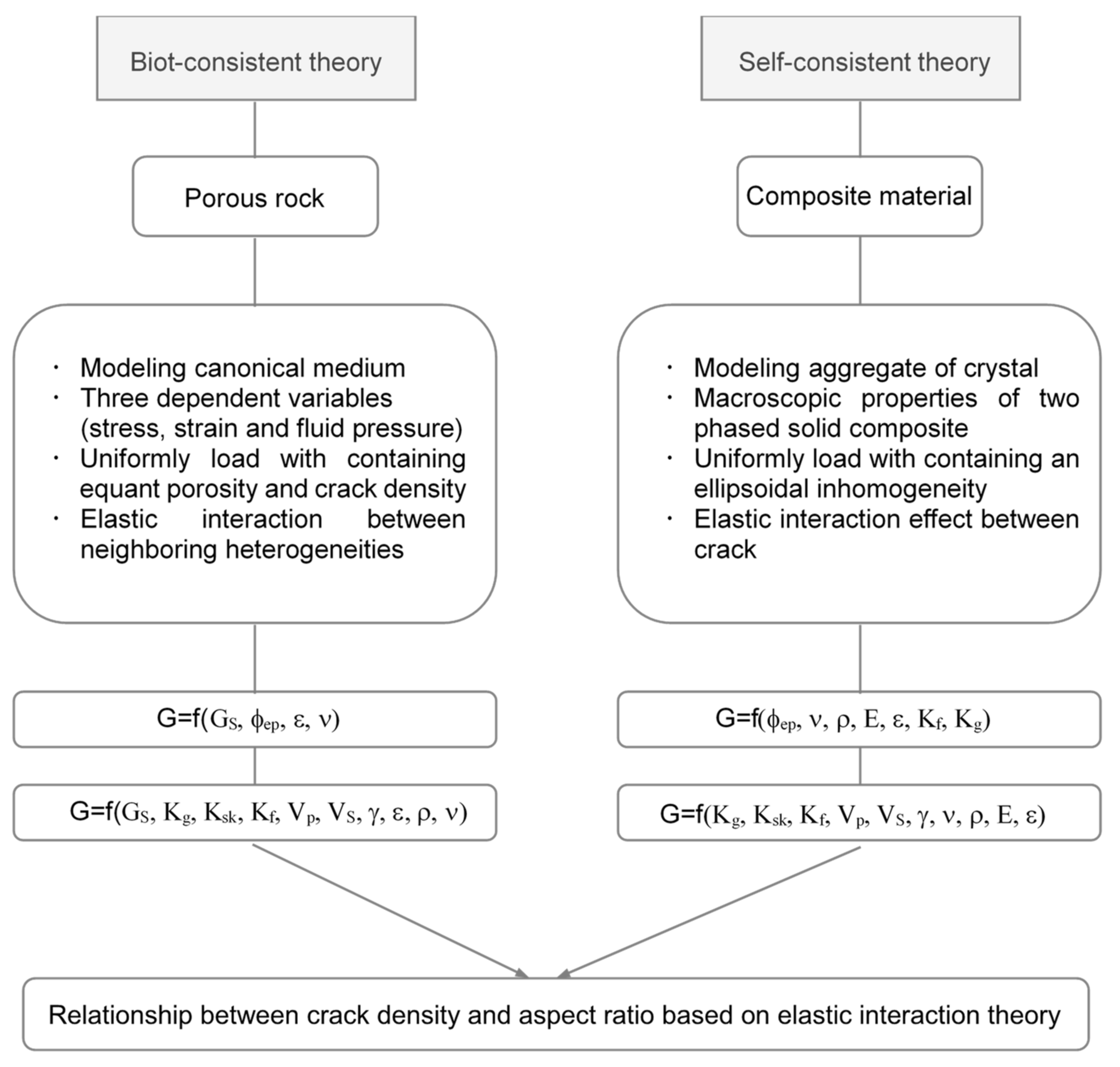
2.1. Aspect Ratio and Crack Density

Biot [22] introduced the theory of wave propagation in porous media and defined constitutive equations for stress, strain, and elastic moduli. These variables have a linear relationship in elastic materials, as this theory assumes that the wave-propagating medium is homogeneous, isotropic, and un-cracked. In addition, pore water pressure is assumed constant in all directions. As a result, this theory has limited applicability to heterogeneous materials that may contain many cracks. This theory was then developed further to generate a new Biot-consistent theory that related explicitly to porous rocks, as shown in Figure 1 [22,23]. This Biot-consistent theory uses three dependent variables (stress, strain, and fluid pressure) to model a canonical medium in which porosity and crack density are isotropic. Equant porosity (ϕ_ep) and crack density (ε) are then defined in terms of the shear modulus (G), as follows:

$$\mathrm{G}={\mathrm{G}}_{\mathrm{s}}\left[1-\frac{{\varnothing }_{\mathrm{ep}}}{1-\left(\frac{2}{15}·\frac{4-5\mathsf{\nu }}{1-\mathsf{\nu }}\right)}-\left(\frac{32}{45}·\frac{\left(1-\mathsf{\nu }\right)\left(5-\mathsf{\nu }\right)}{\left(2-\mathsf{\nu }\right)}\right)\mathsf{\epsilon }\right]$$

(1)

where G_s is the shear modulus of a grain and ν is Poisson’s ratio.

An alternative technique for investigating crack development in a composite material is self-consistent theory [24,25]. The theory is generally used to model aggregates of crystals and can quantify the macroscopic properties of two-phase solid composites. This theory assumes that a load is uniformly applied to an ellipsoidal, heterogeneous material. Kachanov [26] expanded this theory to consider polarization of fluid pressure, allowing this self-consistent theory to be applied to cracks and pores in a specific effective medium (CPEM), such as a porous-cracked rock [13]. The value of G in CPEM is defined as follows:

$$\mathrm{G}=2+\left[\frac{{\varnothing }_{\mathrm{ep}}·15·(1-\left(1-\mathsf{\nu }\right)}{7-5\mathsf{\nu }}\right]+\mathsf{\rho }\left[\frac{16\left(1-\mathsf{\nu }\right)}{15\left(1-\frac{\mathsf{\nu }}{2}\right)}+32\frac{\left(1-\mathsf{\nu }\right)\left[\mathrm{E}\mathsf{\pi }·\frac{\mathsf{\epsilon }}{4\left(1-{\mathsf{\nu }}^2\right)}·\left(\frac{1}{{\mathrm{K}}_{\mathrm{f}}}-\frac{1}{{\mathrm{K}}_{\mathrm{g}}}\right)\right]}{45·\left[1+\mathrm{E}\mathsf{\pi }·\frac{\mathsf{\epsilon }}{4\left(1-{\mathsf{\nu }}^2\right)}·\left(\frac{1}{{\mathrm{K}}_{\mathrm{f}}}-\frac{1}{{\mathrm{K}}_{\mathrm{g}}}\right)\right]}\right]$$

(2)

where K_f and K_g are the bulk moduli of fluids and grains, respectively; E is the Young’s modulus of the material; ν is Poisson’s ratio, ϕ_ep is equant porosity; and ε is crack density. In a cracked medium, the total porosity (ϕ), as shown in Equation (3) consists of an equant porosity (ϕ_ep) and a crack porosity (ϕ_cp). The aspect ratio (ρ), which is the ratio of the lengths of the shortest to the longest axes of an object, is used to classify porosity. The aspect ratio is >0.1 for equant porosity and ≤0.1 for crack porosity [27]. The crack porosity may be re-expressed in terms of crack density and aspect ratio, as follows:

$$\varnothing ={\varnothing }_{\mathrm{ep}}+{\varnothing }_{\mathrm{cp}}={\varnothing }_{\mathrm{ep}}+\frac{4}{3}\mathsf{\pi }\mathsf{\rho }\mathsf{\epsilon }$$

(3)

Crack density is mathematically defined by the representative elementary volume (V), the length of a spheroid semi-axis (c), and the number of cracks (n) in a material, as shown in Equation (4):

$$\mathsf{\epsilon }=\frac{1}{\mathrm{V}}{\displaystyle \sum }_{\mathrm{i}}^{\mathrm{n}}{\mathrm{C}}_{\mathrm{i}}^3$$

(4)

The total porosity can be determined by using elastic moduli and the theory of wave propagation suggested by Biot [22] with such a relationship having already been applied to various materials, including rock, sand, silty sand, silty clay, silt, and clay-sand mixtures [28]. This Equation for total porosity is given as follows:

ϕ = f(K_g, K_sk, K_f, V_p, V_S, γ)

(5)

where K_g, K_sk, and K_f are the bulk moduli of a grain, skeleton, and fluid, respectively; V_P and V_S are compressional and shear wave velocities, respectively; and γ is the mass density.

As such, the parameters for shear moduli based on both Biot-consistent (G_{Biot-consistent}) and self-consistent (G_{self-consistent}) theories may be evaluated through Equations (3) and (5), to produce the following:

G_{Biot-consistent} = f(G_S, ϕ_ep, ε, ν) = f(G_S, ϕ, ε, ρ, ν) = f(G_S, K_g, K_sk, K_f, V_p, V_S, γ, ε, ρ, ν)

(6)

G_{self-consistent} = f(ϕ_ep, ν, ρ, E, ε, K_f, K) = f(ϕ, ν, ρ, E, ε, K_f, K) = f(K_g, K_sk, K_f, V_p, V_S, γ, ν, ρ, E, ε, K)

(7)

Equations (6) and (7) thus define crack density as a function of compressional (V_p) and shear (V_s) wave velocities, which has prompted various researchers to estimate ε in a material by measuring its elastic wave velocity, mass density, and assumed bulk moduli. However, the exact crack density is difficult to determine, as the aspect ratio remains unknown; an independent technique is therefore necessary to define its value. Although Equations (1) and (2) were developed using different theoretical backgrounds, both consider elastic interactions, and so here we establish a new relationship between the unknown parameters of crack density and aspect ratio by combining the two Equations.

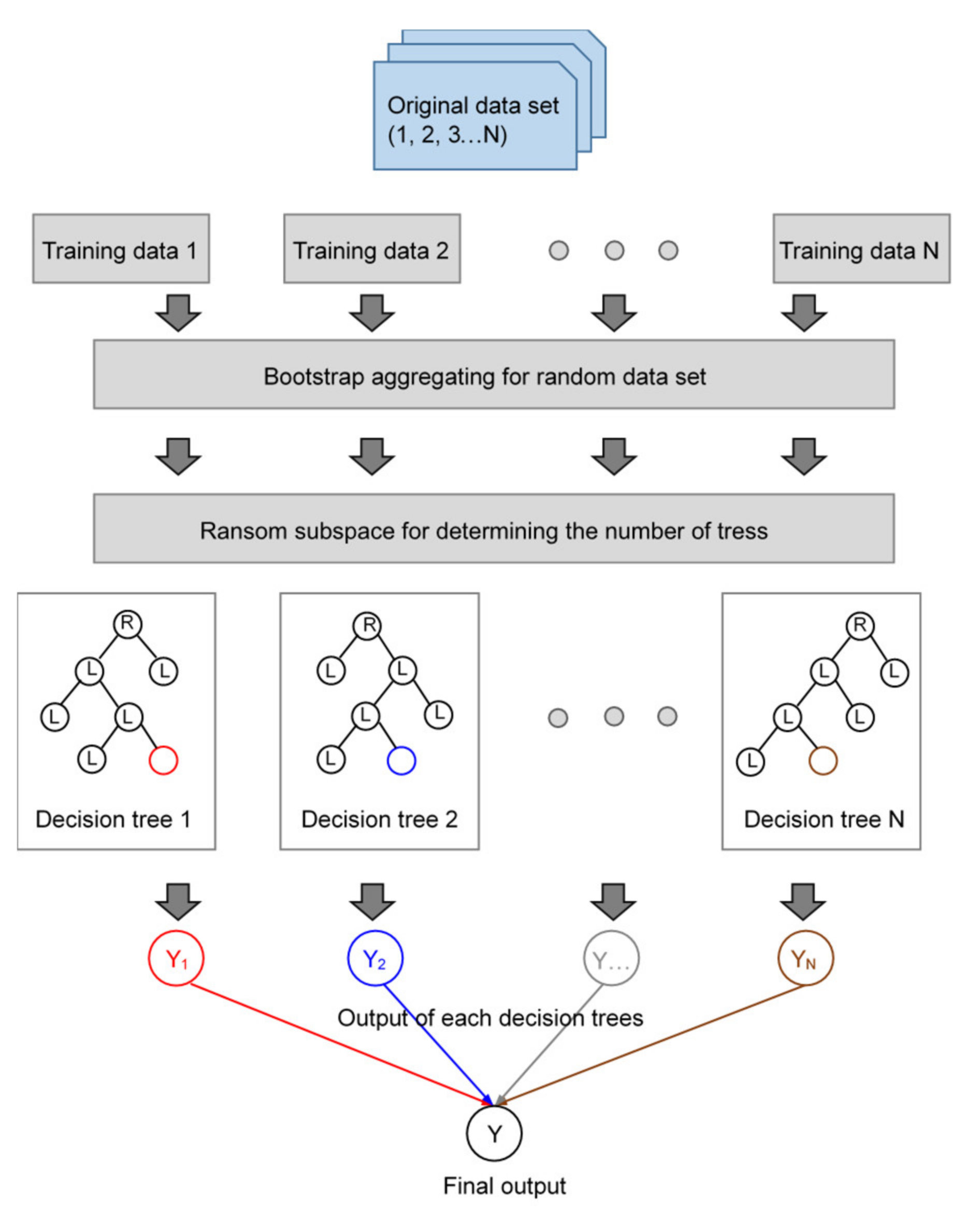
2.2. Random Forest Algorithm

The decision tree is one of the ML techniques that can provide classification and regression by dividing the pattern of data step by step in the form of tree branches. If the data is plotted in two-dimensional of x-axis and y-axis, the analysis can be visually performed through graphs and however, it is difficult to directly understand the graph when there are many variables. Thus, the decision tree based on binary classifier is used. Even though this method has an advantage of easily checking the data structure, it has limitation to increase reliability because the error is continuously accumulated to a next level. The final value, which is affected by small noise, may be biased due to characterization of architecture in decision tree. To improve the disadvantage, the algorithm of random forest (RF) was suggested. Even though the principle and architecture of RF is similar with decision tree, RF constructs the forest with various numbers of trees as an ensemble technique [29]. In RF, the bootstrap aggregating method is applied to create multiple training data sets from the same variable as shown in Figure 2. This method allows overlap when selecting data as sampling with replacement to have an equal size with the number of original data. The random subspace is also applied to determine the number of trees, and the various leaf nodes are divided from root node considering minimization of cost function. The various number of trees suppress overfitting occurred in the general decision tree using only one tree by strong law of large numbers. The input variable, that is not selected in bootstrap aggregating, is used as validation data to verify the reliability of constructed RF, and it is called to out of bag (OOB). The data sets can be randomly mixed to analyze the importance of each variable. If the errors based on OOB of original data and randomly mixed data are expressed by e_i and r_i, the important score among input variables can be calculated through Equation (8).

$${\mathrm{v}}_{\mathrm{i}}=\frac{\frac{1}{\mathrm{t}}{{\displaystyle \sum }}_{\mathrm{i}=1}^{\mathrm{t}}\left|{\mathrm{e}}_{\mathrm{i}}-{\mathrm{r}}_{\mathrm{i}}\right|}{\sqrt{\frac{1}{\mathrm{t}-1}{{\displaystyle \sum }}_{\mathrm{i}=1}^{\mathrm{t}}{[\left(\left|{\mathrm{e}}_{\mathrm{i}}-{\mathrm{r}}_{\mathrm{i}}\right|\right)-(\frac{1}{\mathrm{t}}{{\displaystyle \sum }}_{\mathrm{i}=1}^{\mathrm{t}}\left|{\mathrm{e}}_{\mathrm{i}}-{\mathrm{r}}_{\mathrm{i}}\right|)]}^2}}$$

(8)

The grey relational grade (GRG) has been applied to find the numerical correlations between two variables and it can be calculated through Equation (9) based on referencing (X_R) and comparing (X_C) variables.

$$\mathrm{GRG}=\frac{1}{\mathrm{n}}{\displaystyle \sum }_{\mathrm{j}=1}^{\mathrm{n}}\frac{\underset{\mathrm{i}}{\min }\underset{\mathrm{j}}{\min }\left|{\mathrm{X}}_{\mathrm{R},\mathrm{j}}-{\mathrm{X}}_{\mathrm{C},\mathrm{j}}\right|+\mathsf{\delta }\underset{\mathrm{i}}{\max }\underset{\mathrm{j}}{\max }\left|{\mathrm{X}}_{\mathrm{R},\mathrm{j}}-{\mathrm{X}}_{\mathrm{C},\mathrm{j}}\right|}{\left|{\mathrm{X}}_{\mathrm{R},\mathrm{j}}-{\mathrm{X}}_{\mathrm{C},\mathrm{j}}\right|+\mathsf{\delta }\underset{\mathrm{i}}{\max }\underset{\mathrm{j}}{\max }\left|{\mathrm{X}}_{\mathrm{R},\mathrm{j}}-{\mathrm{X}}_{\mathrm{C},\mathrm{j}}\right|}$$

(9)

where j is sequence of each variable. The δ denotes the resolving coefficient and the value is generally assumed to 0.5 [30].

2.3. Sensitivity Analysis of Each Theory

Equations (1) and (2) may be rearranged in terms of crack density; crack density is calculated by changing the only selected parameter with constant left parameters. The ratio of change may decrease or increase by up to 100% based on the true value, which can be found in the literature (e.g., Byun et al. [4]). Representative values are summarized in

Table 1. True value for sensitivity analysis obtained by Byun et al. [4].

Input Parameter	Symbol	Value	Unit
Compressional wave velocity	VP	3837	m/s
Shear wave velocity	VS	2213	m/s
Mass density	γ	2800	kg/m3
Poisson’s ratio	ν	0.1	-
Bulk modulus of grain	Kg	15,000,000,000	Pa
Bulk modulus of skeleton	Ksk	7,780,000	Pa
Bulk modulus of fluid	Kf	2,180,000,000	Pa
Shear modulus of grain	GS	13,000,000,000	Pa
Aspect ratio	ρ	0.19	-

. Finally, sensitivity analysis was performed using Equation (10):

$$\mathrm{Sensitivity}=\frac{{\mathrm{CR}}_{\mathrm{true}}-{\mathrm{CR}}_{\mathrm{calculated}}}{{\mathrm{CR}}_{\mathrm{calculated}}}$$

(10)

where CR_true is the true crack density obtained from true input parameters, and CR_calcualted is the calculated crack density obtained by changing these input parameters. Sensitivity analysis was performed on the variables that form terms in both Equations (1) and (2): compressional wave velocity, shear wave velocity, mass density, Poisson’s ratio, bulk modulus of a grain, bulk modulus of the skeleton, bulk modulus of a fluid, shear modulus, and crack aspect ratio. The results of sensitivity testing for these nine parameters are shown in the Figure 3. The most influential factors in Equation (1) were the bulk modulus of the fluid and the aspect ratio, whereas the shear modulus was most influential in Equation (2), as shown by a sensitivity value of around 100. The skeleton bulk modulus has the smallest influence in both Equations (1) and (2). Based on these results, parameters may be listed in order of importance for Equations (1) and (2), as follows: ρ > K_f > K_g > γ ≈ ν ≈ G_S > V_P ≈ V_S > K_sk and G_S > γ ≈ K_g > V_P ≈ V_S > ρ > ν ≈ K_f ≈ K_sk, respectively. As each theory uses a different set of background assumptions to derive its Equations, the results of sensitivity analysis also show different patterns; thus, it is non-trivial to physically connect both theories. This limitation was solved by establishing a relationship between crack density and aspect ratio based on the measured values in each Equation. Consequently, crack density or aspect ratio can be calculated by solving two simultaneous Equations.

3. Methodology

3.1. Rock Sample Characterization

Rock samples were collected from 10 different outcrops in south Korea to perform weathering experiments. X-ray diffraction (XRD) was performed on each sample at the Institute for Basic Science, Korea, to characterize their mineral contents. Experimental results are shown in Figure 4 and the mineral composition of each sample is summarized in Figure 5, which presents the proportions of the three most abundant minerals in each case, among albite, biotite, calcite, chlorite, dolomite, hematite, hornblende, magnetite, microcline, muscovite, orthoclase, and/or quartz. Following the sample order shown in Figure 5, the most abundant mineral in each rock was albite (42.4%), albite (52.9%), albite (28.2%), albite (39.4%), quartz (68.6%), quartz (49.2%), quartz (43.4%), biotite (30.6%), calcite (97.4%), and chlorite (26%). Each rock was named according to the most abundant mineral constituent. Although 10 different sites were examined to reflect the variability of specimens throughout the study region, albite, quartz, biotite, calcite, and chlorite formed the main mineral constituents in most cases. Each sample was extracted in the shape of a cylinder with a diameter of 46 mm, and was subsequently abraded to a length of 30 mm in order to promote the weathering procedure and effectively measure elastic wave velocities.

3.2. Weathering Experiments

Artificial weathering experiments were performed to quantify how crack density changed over time in each rock type. While many factors cause weathering in rocks [31,32], chemical and physical processes were focused upon for convenience. The techniques reported by Byun et al. [4] were considered to accelerate artificial weathering herein. Chemical weathering was performed by immersing each abraded rock in a 2.5 M salty solution for 15 h, which allowed the brine to penetrate the pore space. Afterwards, each sample was dried at ~105 °C for 3 h to induce salt crystal nucleation inside the column, which was then left at room temperature (~22 °C) for 1 h to allow the salt crystals to grow. Each column was then immersed in saltwater for another 3 h and dried again at room temperature for 2 h. Each cycle of chemical weathering lasted for 24 h. Physical weathering was simulated by using a slake durability instrument to generate friction, which involved placing all 10 columns of rock into a drum that was rotated for a 10 min period at ~20 rpm. See Deo [33] for further information about the slake durability instrument and weathering procedure.

3.3. Measurement Techniques

A single set of chemical and physical weathering processes comprised three mechanical weathering cycles and one cycle of chemical weathering. All samples were subjected to three complete sets, and so experienced a total of three chemical weathering cycles and nine mechanical weathering cycles. Therefore, each rock was affected by 12 weathering events in total. In this study, the elastic wave velocity, which is a function of the elastic modulus, was measured to estimate the crack density using the elastic modulus, as defined in Equations (6) and (7). After each weathering cycle, transducers were attached to the upper and lower parts of the rock cylinder, and the compressional and shear waves were measured by the transmission method. The input signal for the elastic wave was propagated using a signal generator (Agilent 33220A) that produced a sine wave with a frequency of 20 Hz. Random noise within the output signal was removed by filtering and amplifying using a Krohn-hite 3364. The low- and high-pass filters utilized had frequencies of 500 Hz and 20 kHz, respectively.

4. Results and Discussion

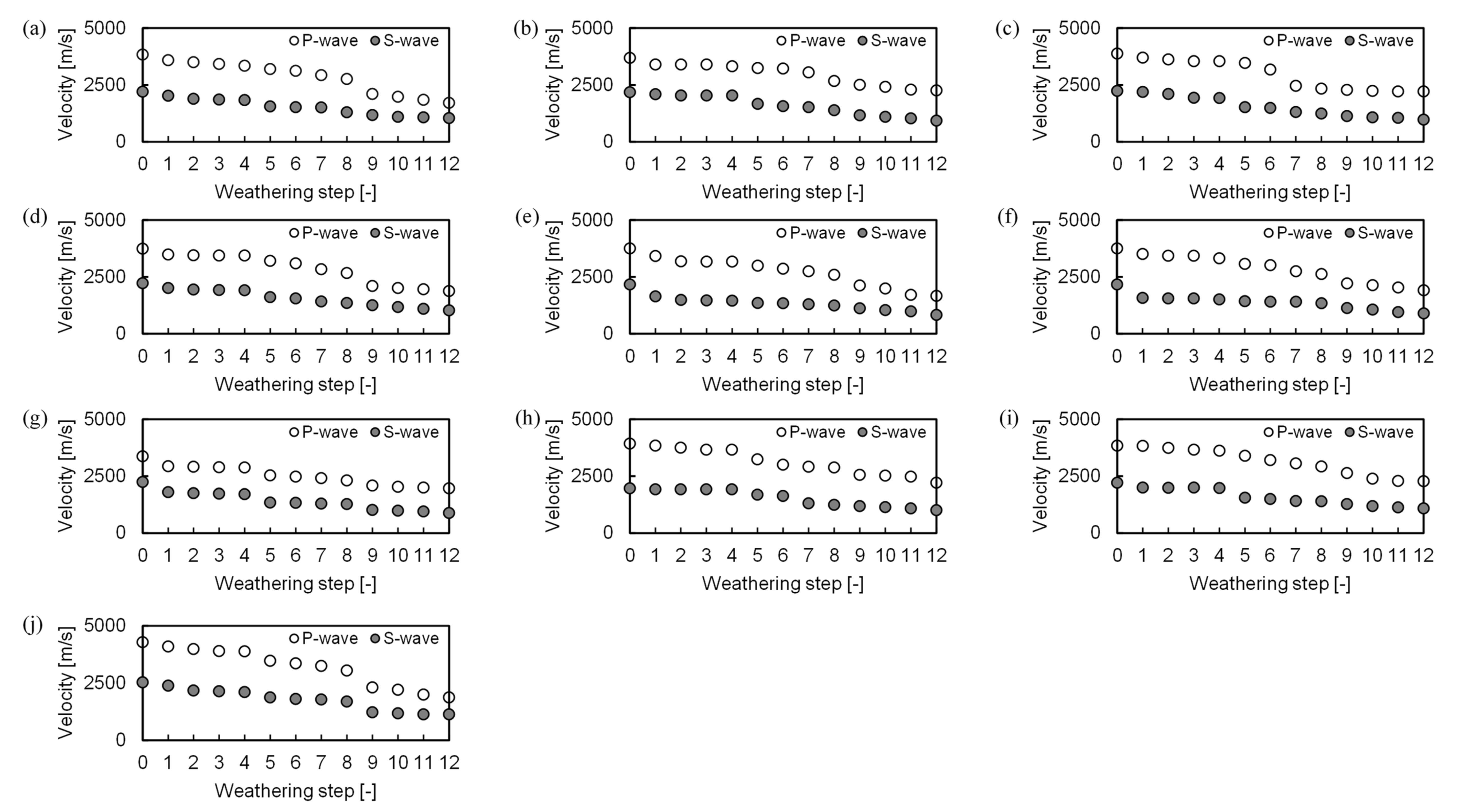
4.1. Elastic Wave Velocity

Measured compressional and shear wave velocities for all 10 unaltered samples lie within the ranges 3375–4277 m/s and 1964–2534 m/s, respectively. Specimen-specific compressional wave velocities are as follows: albite 1 = 3837 m/s, albite 2 = 3697 m/s, albite 3 = 3886 m/s, albite 4 = 3745 m/s, quartz 1 = 3754 m/s, quartz 2 = 3,748 m/s, quartz 3 = 3375 m/s, biotite = 3928 m/s, calcite = 3837 m/s, and chlorite = 4277 m/s. Specimen-specific shear wave velocities are as follows: albite 1 = 2213 m/s, albite 2 = 2190 m/s, albite 3 = 2,242 m/s, albite 4 = 2222 m/s, quartz 1 = 2166 m/s, quartz 2 = 2162 m/s, quartz 3 = 2250 m/s, biotite = 1964 m/s, calcite = 2215 m/s, and chlorite = 2534 m/s. It is notable that the elastic wave velocity of chlorite is relatively high compared to that of quartz and biotite. Figure 6 shows that the elastic wave velocity in each sample gradually decreased as chemical and physical weathering proceeded. Post-weathering bulk compressional and shear wave velocities for all samples changed to 1665–2274 m/s and 832–1131 m/s, respectively. Specimen-specific reductions for compressional wave velocities are as follows: albite 1 = 55%, albite 2 = 38%, albite 3 = 43%, albite 4 = 50%, quartz 1 = 56%, quartz 2 = 49%, quartz 3 = 42%, biotite = 44%, calcite = 41%, and chlorite = 56%. Equivalent percentage decreases for shear wave velocities are as follows: albite 1 = 52%, albite 2 = 56%, albite 3 = 56%, albite 4 = 54%, quartz 1 = 62%, quartz 2 = 59%, quartz 3 = 61%, biotite = 49%, calcite = 51%, and chlorite = 55%.

While compressional waves can propagate through fluids (e.g., air, water) and solids (e.g., minerals), shear waves can only be transmitted through the latter, making them useful for determining fabric characteristics within a rock [34,35]. Reductions in compressional and shear wave velocities due to weathering (Figure 7) can be calculated via subtraction of a sample’s pre- to post-weathering shear wave reduction from a sample’s pre- to post-weathering compressional wave reduction. The average difference in reduction ratio for all 10 samples was approximately −8%, with the negative sign showing that weathering reduced the shear wave velocity to a proportionally greater degree than the compressional wave velocity. Both albite 2 and quartz 3 samples showed the greatest magnitude of change (around −19%), which infers a high biotite (Mohs hardness scale ≈ 2.5) and orthoclase (Mohs hardness scale ≈ 6) content in each, giving the rocks an average Mohs hardness scale value of around 4 (cf. Figure 5). Of the samples albite 1, albite 2, albite 3, and albite 4, which have high albite content, albite 2 had the highest reduction ratio of −18%, because it has relatively sparse quartz (20.9%), which has a high Mohs hardness scale value of around 7, and relatively abundant biotite (10.7%), which has a low Mohs hardness scale value of around 2.5. Of the samples quartz 1, quartz 2, and quartz 3, the reduction ratio for quartz 2 was greatest (−18%) due to its relatively sparse quartz (Mohs hardness scale ≈ 7) and abundant orthoclase (Mohs hardness scale ≈ 6).

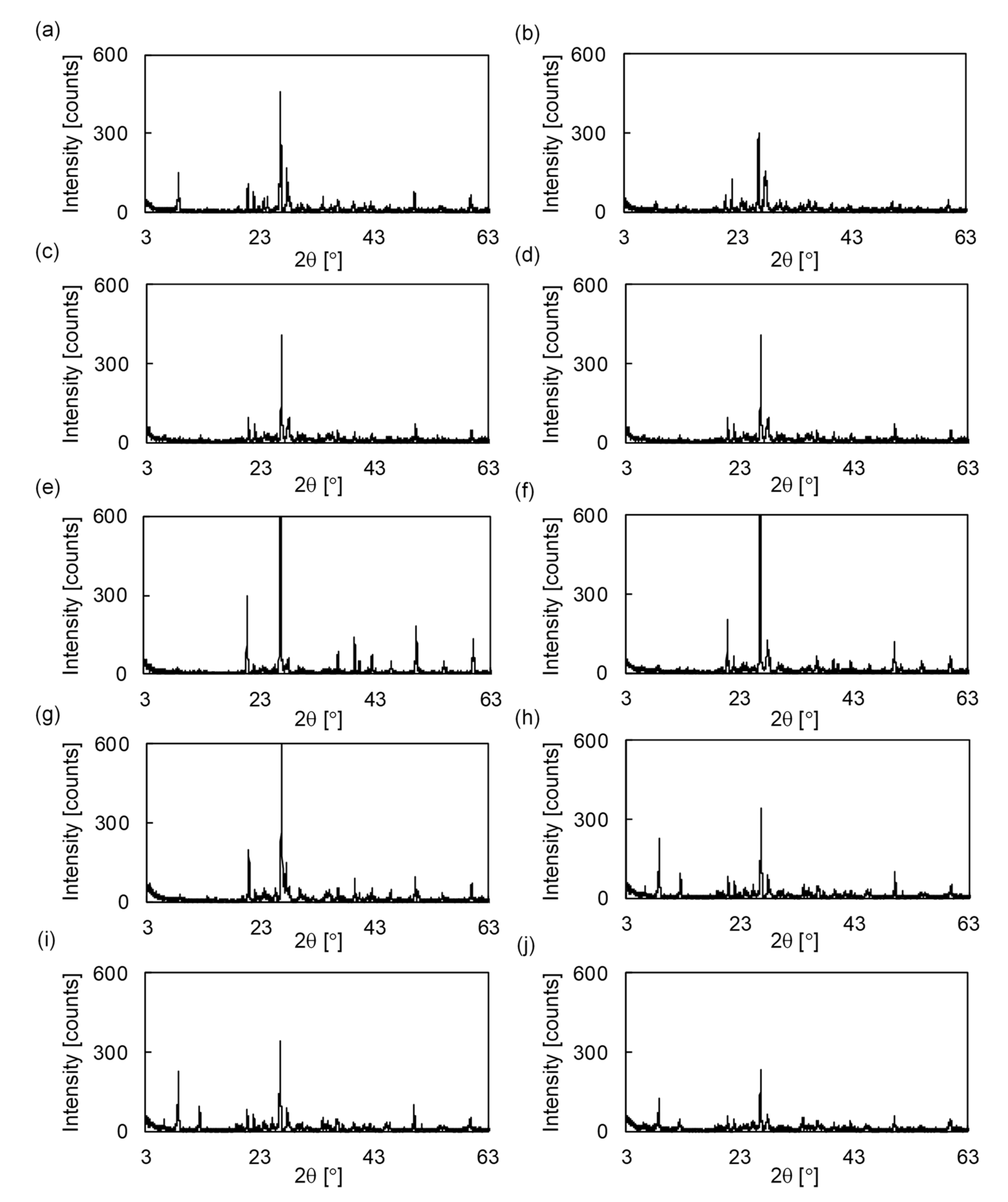
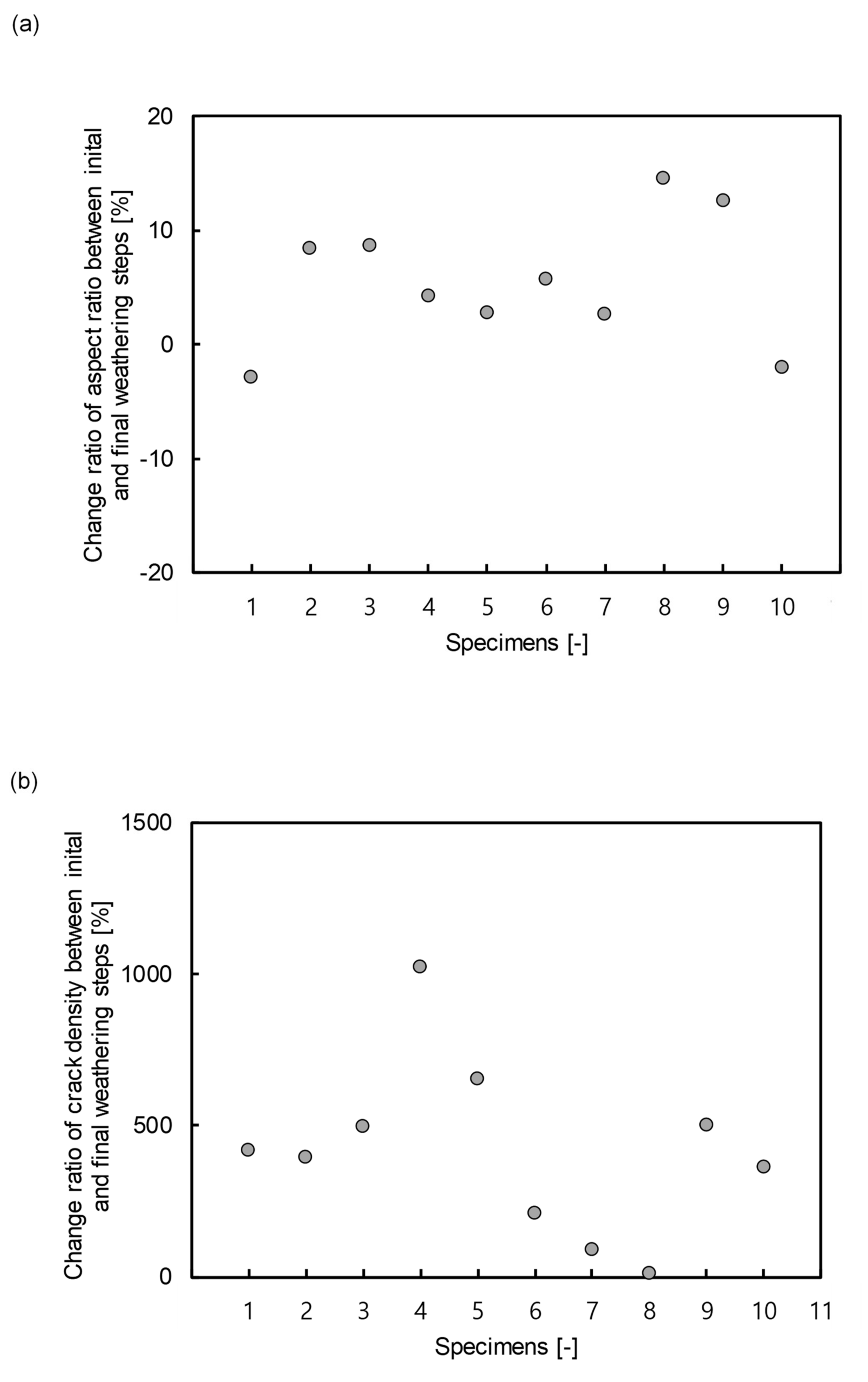
4.2. Quantifying Aspect Ratio and Crack Density

The measured elastic wave velocities for each sample were substituted in Equations (1) and (2) to produce two separate equations parameterized with only aspect ratio and crack density as unknowns. Both of these resultant equations were combined and solved simultaneously to obtain sample-specific aspect ratio and crack density values, which are shown in Figure 8 and Figure 9. Equations (6) and (7) show that Equations (1) and (2) can be reformulated simply using the relationship between the elastic wave velocity and the porosity, which contains 10 different parameters. The measured values were used for elastic wave velocities, and both Young’s modulus (E) and Poisson’s ratio (ν) were calculated in terms of compressional (V_p) and shear wave (V_S) velocities, as shown in Equations (11) and (12):

$$v=\frac{{\mathrm{Vp}}^2-2{\mathrm{Vs}}^2}{2\left({\mathrm{Vp}}^2-{\mathrm{Vs}}^2\right)}$$

(11)

$$\mathrm{E}=\frac{-4{\mathrm{Vs}}^4\gamma -3{\mathrm{Vp}}^2{\mathrm{Vs}}^2\gamma }{{\mathrm{Vp}}^2-{\mathrm{Vs}}^2}$$

(12)

The bulk moduli for grain (K_g), skeleton (K_sk), and fluid (K_f) phases in all samples were assumed to be 15 × 109 Pa, 7.78 × 106 Pa, and 2.18 × 109 Pa, respectively, as reported by Lee and Yoon [35]. The grain (G_s) shear modulus and mass density (γ) were assumed to be 13 × 109 Pa and 2800 kg/m³, respectively [4]. Unaltered rock columns had calculated aspect ratios and crack densities in the ranges 0.1872–0.1948 and 0.1829–0.2120, respectively, although post-weathering values changed to 0.014–0.133 and 0.1131–0.2220, respectively. Figure 10 shows absolute change ratios based on pre- and post-weathering values of aspect ratio and crack density. These change ratios are −2–14% and 9–1021%, respectively, revealing that crack density showed a significantly greater difference due to weathering, whereas the aspect ratio remained almost constant. Fortin et al. [36] suggested similar behavior during an increase in effective stress (i.e., the aspect ratio of a rock remains constant despite the crack density changing). The number of cracks per unit volume thus increases as weathering progresses, which greatly influences the crack density. However, the aspect ratio of a crack, which is the ratio of its short and long dimensions, shows a relatively small percentage change because simply opening a crack via weathering does not change its longitudinal and transverse orientations.

Unlike the elastic wave velocity, it is difficult to determine a sample’s tendency of composed mineral via calculation of aspect ratio and crack density. The total porosity (ϕ) consists of equant porosity (ϕ_ep) and crack porosity (ϕ_cp), and the relative proportions of both in most rocks are thought to be about 95% and 5%, respectively [37,38]. Therefore, the total porosity is often dependent on the equant porosity, which influences elastic wave propagation. Further, elastic wave velocity shows a good tendency with composed mineral in specimens as the weathering process continues. Nonetheless, aspect ratio and crack density limit our ability to characterize some sample properties, such as seismic velocity, as they are related to equant porosity, which forms a relatively small proportion of the total porosity and only weakly influences microstructural behaviors.

4.3. Importance of Each Variable Based on Random Forest

RF algorithm was used to examine the effects of input variables on aspect ratio and crack density. The 130 data set including compressional wave velocity, shear wave velocity, total porosity, crack porosity, equant porosity, derived during 13 weathering processes in 10 rocks, was used. The selected input variables are normalized through the technique of min-max scaling, as shown in Equation (13), to remove the bias that occurred by magnitude and unit of variables, and thus the data set was normalized in the range of −1 to 1.

$${\mathrm{RF}}_{\min -\max \mathrm{scaling}}=\left(\frac{\mathrm{IV}-{\mathrm{IV}}_{\min }}{{\mathrm{IV}}_{\max }-{\mathrm{IV}}_{\min }}\right)\left(\overline{{\mathrm{IV}}_{\max }}-\overline{{\mathrm{IV}}_{\min }}\right)+\overline{{\mathrm{IV}}_{\min }}$$

(13)

where IV denotes the input variable. The IV_max and IV_min mean the maximum and minimum values of input variable. The $\overline{{\mathrm{IV}}_{\max }}$ and $\overline{{\mathrm{IV}}_{\min }}$ are −1 and 1, respectively.

The number of random data set and tree were determined to 20 and 10 under the condition that the accuracy is 0.876. The accuracy was calculated with true positive (TP), false positive (FP), false negative (FN), and true negative (TN) through Equation (14).

$$\mathrm{Accuracy}=\frac{\left(\mathrm{TP}+\mathrm{TN}\right)}{\left(TP+TN+FP+FN\right)}$$

(14)

The important score of each variable for estimating aspect ratio is calculated by using Equation (8) and it was addressed in Figure 11. The highest affecting parameters to determine aspect ratio are crack density (0.32 point), crack density (0.35 point), total porosity (0.37 point), crack density (0.27 point), shear wave velocity (0.32 point), equant porosity (0.37 point), crack porosity (0.18 point), crack density (0.16 point), crack porosity (0.45 point) and crack porosity (0.45 point) for albite 1, albite 2, albite 3, albite 4, quartz 1, quartz 2, quartz 3, biotite, calcite, and chlorite, respectively. The important scores were calculated considering overall characteristics of the variables since there are various variables to derive the aspect ratio. Although the factors with high scores were slightly different for characterization of each rock, the factors that had the highest influence on the aspect ratio through averaged points were in the order of crack porosity (0.20 point) > total porosity (0.19 point) > shear wave (0.16 point) > crack density (0.15 point) > equant porosity (0.12 point) > compressional wave (0.10 point).

The GRG was selected to find the correlation between pairwise variables of aspect ratio, crack density, compressional wave velocity, shear wave velocity, total porosity, crack porosity and equant porosity. The Figure 12 shows the GRG value in each panel and, the mean, minimum and maximum values of GRG are 0.52, 0.99, and 0.1, respectively. It indicates the crack porosity is the most significant effect on both crack density and aspect ratio. It shows that the accuracy of crack porosity is important to obtain a reliable aspect ratio and crack density.

4.4. Relationship between Aspect Ratio and Crack Density

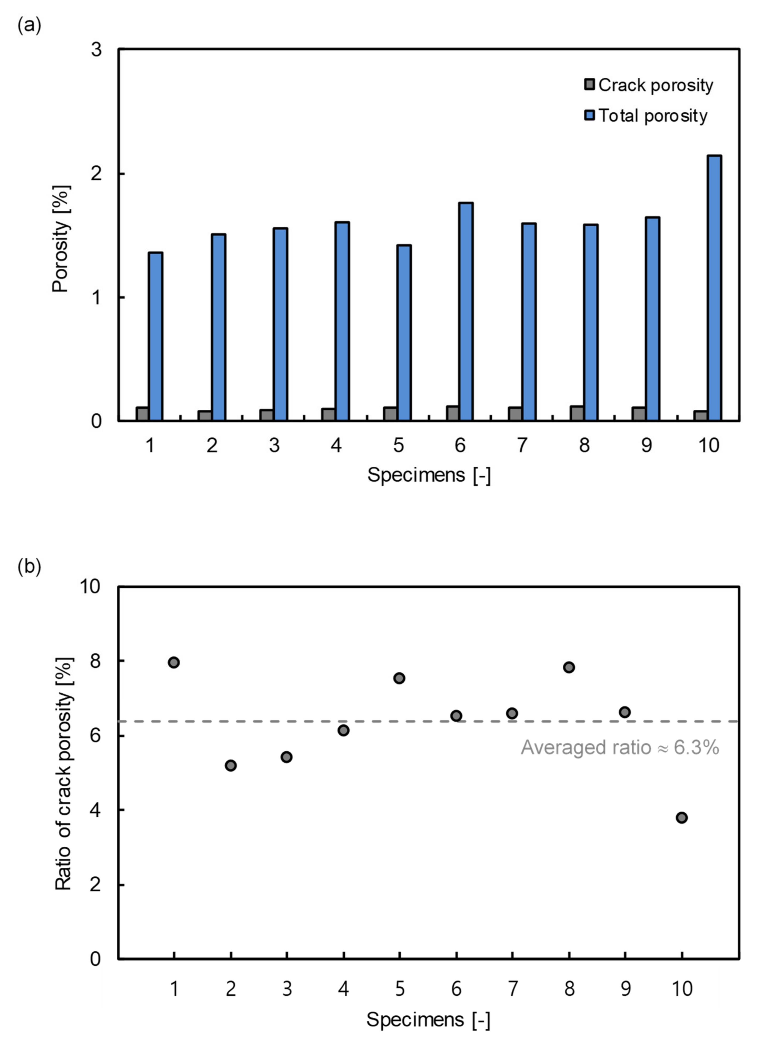
Individual equations for aspect ratio and crack density were combined in this work to form a single relationship between both parameters based on exponential function (Figure 13). The mathematical relationship between aspect ratio and crack density is shown in Equation (15).

$$\mathrm{Aspect}\mathrm{ratio}=0.1625e^{\left(14.989*crack density\right)}, R^2=0.8837$$

(15)

The aspect ratio and crack density values, studied by Endres and Knight [39], Adelinet et al. [13], and Fortin et al. [36], are also described in Figure 13 and they are mostly included in the trend line proposed in this study. However, Equation (15) has a limitation in explaining the deviation of aspect ratio in the range of 0.15–0.2 in crack density, and thus more data are necessary to understand the behavior.

4.5. Verification

To verify the reliability of specimen-specific calculated aspect ratio and crack density values, both the total porosity and crack porosity of that specimen were calculated. The weight and volume of each specimen were measured to determine the total porosity created during the weathering process, and crack porosity was calculated using the aspect ratio and crack density values substituted into Equation (3). The calculated porosity at each step was averaged and the results shown in Figure 14. The calculated total porosity and crack porosity were in the ranges 1.36–2.14% and 0.083–0.124%, respectively, and the crack porosity had a relatively small absolute value. The calculated ratio of crack porosity to total porosity is shown in Figure 14b, and had a range of 3.8–7.9% and a mean value of ~6.3%. This result matches those of previous studies, which suggest that crack porosity accounts for about 5% of the total porosity [37,38], showing that the aspect ratios and crack densities derived from the Equations presented in this work are reliable.

5. Conclusions

In this study, a relationship between crack aspect ratio and crack density was derived through combination of several constitutive equations, and subsequently verified by matching predicted and observed results from weathering experiments. The detailed conclusions that can be drawn from this study are summarized below.

• Various parameters included in two constitutive equations were rearranged and simplified to define elastic wave velocity, with aspect ratio and crack density as the main variables to be solved.
• Ten rock columns were each subjected to three chemical and nine physical experimental weathering cycles. The elastic wave velocity was continually measured in each column, allowing predictions of their evolving aspect ratio and crack density.
• The reliability of the calculated aspect ratio and crack density data was verified by measuring the ratio of crack porosity to total porosity. These data allowed for the formulation of a relationship between aspect ratio and crack density that may be applied to a broad spectrum of samples.

References

1. Tuǧrul, A. The effect of weathering on pore geometry and compressive strength of selected rock types from Turkey. Eng. Geol. 2004, 75, 215–227. [Google Scholar] [CrossRef]
2. Wang, P.; Xu, J.; Liu, S.; Wang, H.; Liu, S. Static and dynamic mechanical properties of sedimentary rock after freeze-thaw or thermal shock weathering. Eng. Geol. 2016, 210, 148–157. [Google Scholar] [CrossRef] [Green Version]
3. Palmstrom, A. RMi-a Rock Mass Characterization System for Rock Engineering Purposes. Ph.D. Thesis, University of Oslo, Oslo, Norway, 1995. [Google Scholar]
4. Byun, J.H.; Lee, J.S.; Park, K.; Yoon, H.K. Prediction of crack density in porous-cracked rocks from elastic wave velocities. J. Appl. Geophys. 2015, 115, 110–119. [Google Scholar] [CrossRef]
5. Nasseri, M.H.B.; Schubnel, A.; Young, R.P. Coupled evolutions of fracture toughness and elastic wave velocities at high crack density in thermally treated Westerly granite. Int. J. Rock Mech. Min. Sci. 2007, 44, 601–616. [Google Scholar] [CrossRef]
6. Biot, M.A. General theory of three-dimensional consolidation. J. Appl. Phys. 1941, 12, 155–164. [Google Scholar] [CrossRef]
7. Bristow, J.R. Microcracks, and the static and dynamic elastic constants of annealed and heavily cold-worked metals. Br. J. Appl. Phys. 1960, 11, 81. [Google Scholar] [CrossRef]
8. Walsh, J.B. New analysis of attenuation in partially melted rock. J. Geophys. Res. 1969, 74, 4333–4337. [Google Scholar] [CrossRef]
9. Garbin, H.D.; Knopoff, L. The compressional modulus of a material permeated by a random distribution of circular cracks. Q. Appl. Math. 1973, 30, 453–464. [Google Scholar] [CrossRef] [Green Version]
10. Budiansky, B.; O’Connell, R.J. Elastic moduli of a cracked solid. Int. J. Solids Struct. 1976, 12, 81–97. [Google Scholar] [CrossRef]
11. Hill, R. A self-consistent mechanics of composite materials. J. Mech. Phys. Solids 1965, 13, 213–222. [Google Scholar] [CrossRef]
12. Berryman, J.G. Long-wavelength propagation in composite elastic media II. Ellipsoidal inclusions. J. Acoust. Soc. Am. 1980, 68, 1820–1831. [Google Scholar] [CrossRef]
13. Adelinet, M.; Fortin, J.; Guéguen, Y. Dispersion of elastic moduli in a porous-cracked rock: Theoretical predictions for squirt-flow. Tectonophysics 2011, 503, 173–181. [Google Scholar] [CrossRef]
14. Tang, X. A unified theory for elastic wave propagation through porous media containing cracks—An extension of Biot’s poroelastic wave theory. Sci. China Earth Sci. 2011, 54, 1441. [Google Scholar] [CrossRef]
15. Comert, R.; Avdan, U.; Gorum, T.; Nefeslioglu, H.A. Mapping of shallow landslides with object-based image analysis from unmanned aerial vehicle data. Eng. Geol. 2019, 260, 105264. [Google Scholar] [CrossRef]
16. Đurić, U.; Marjanović, M.; Radić, Z.; Abolmasov, B. Machine learning based landslide assessment of the Belgrade metropolitan area: Pixel resolution effects and a cross-scaling concept. Eng. Geol. 2019, 256, 23–38. [Google Scholar] [CrossRef]
17. Lü, Q.; Chan, C.L.; Low, B.K. Probabilistic evaluation of ground-support interaction for deep rock excavation using artificial neural network and uniform design. Tunn. Undergr. Space Technol. 2012, 32, 1–18. [Google Scholar] [CrossRef]
18. Sudakov, O.; Burnaev, E.; Koroteev, D. Driving digital rock towards machine learning: Predicting permeability with gradient boosting and deep neural networks. Comput. Geosci. 2019, 127, 91–98. [Google Scholar] [CrossRef] [Green Version]
19. Karimpouli, S.; Tahmasebi, P. Segmentation of digital rock images using deep convolutional autoencoder networks. Comput. Geosci. 2019, 126, 142–150. [Google Scholar] [CrossRef]
20. Mills, G.; Fotopoulos, G. Rock surface classification in a mine drift using multiscale geometric features. IEEE Geosci. Remote Sens. Lett. 2015, 12, 1322–1326. [Google Scholar] [CrossRef]
21. Qi, C.; Fourie, A.; Du, X.; Tang, X. Prediction of open stope hangingwall stability using random forests. Nat. Hazards 2018, 92, 1179–1197. [Google Scholar] [CrossRef]
22. Biot, M.A. Mechanics of deformation and acoustic propagation in porous media. J. Appl. Phys. 1962, 33, 1482–1498. [Google Scholar] [CrossRef]
23. Biot, M.A.; Willis, D.G. The elastic coeff cients of the theory of consolidation. J. Appl. Mech. 1957, 24, 594–601. [Google Scholar]
24. Hershey, A.V. The elasticity of an isotropic aggregate of anisotropic cubic crystals. J. Appl. Mech. Trans. ASME 1954, 21, 236–240. [Google Scholar]
25. Kröner, E. Berechnung der elastischen Konstanten des Vielkristalls aus den Konstanten des Einkristalls. Z. für Phys. 1958, 151, 504–518. [Google Scholar] [CrossRef]
26. Kachanov, M. Elastic solids with many cracks and related problems. In Advances in Applied Mechanics; Elsevier: Amsterdam, The Netherlands, 1993; Volume 30, pp. 259–445. [Google Scholar]
27. Zhang, J.J.; Bentley, L.R. Pore geometry and elastic moduli in sandstones. CREWES Res. Rep. 2003, 115, 1–20. [Google Scholar]
28. Lee, J.S.; Yoon, H.K. Theoretical relationship between elastic wave velocity and electrical resistivity. J. Appl. Geophys. 2015, 116, 51–61. [Google Scholar] [CrossRef]
29. Breiman, L. Random forest. Mach. Learn. 2001, 45, 5–32. [Google Scholar] [CrossRef] [Green Version]
30. Zhang, P.; Yin, Z.Y.; Jin, Y.F.; Chan, T.H. A novel hybrid surrogate intelligent model for creep index prediction based on particle swarm optimization and random forest. Eng. Geol. 2020, 265, 105328. [Google Scholar] [CrossRef]
31. Liu, Z.; De Schutter, G.; Deng, D.; Yu, Z. Micro-analysis of the role of interfacial transition zone in “salt weathering” on concrete. Constr. Build. Mater. 2010, 24, 2052–2059. [Google Scholar] [CrossRef]
32. Sengun, N.; Demirdag, S.; Ugur, I.; Akbay, D.; Altindag, R. Assessment of the physical and mechanical variations of some travertines depend on the bedding plane orientation under physical weathering conditions. Constr. Build. Mater. 2015, 98, 641–648. [Google Scholar] [CrossRef]
33. Deo, P. Shales as embankment materials. Jt. Highw. Res. Proj. 1972, 45, 100–150. [Google Scholar]
34. Lee, J.S.; Byun, Y.H.; Yoon, H.K. Study of Activation Energy in Soil through Elastic Wave Velocity and Electrical Resistivity. Vadose Zone J. 2017, 16, 1–9. [Google Scholar] [CrossRef]
35. Lee, J.S.; Yoon, H.K. Application example: Field Velocity Resistivity Probe (FVRP) for predicting pore pressure parameter B. Soil Dyn. Earthq. Eng. 2018, 107, 214–217. [Google Scholar] [CrossRef]
36. Fortin, J.; Stanchits, S.; Vinciguerra, S.; Guéguen, Y. Influence of thermal and mechanical cracks on permeability and elastic wave velocities in a basalt from Mt. Etna volcano subjected to elevated pressure. Tectonophysics 2011, 503, 60–74. [Google Scholar] [CrossRef] [Green Version]
37. Sun, Y.F.; Goldberg, D. Estimation of aspect-ratio changes with pressure from seismic velocities. Geol. Soc. Lond. Spec. Publ. 1997, 122, 131–139. [Google Scholar] [CrossRef]
38. Sausse, J.; Jacquot, E.; Fritz, B.; Leroy, J.; Lespinasse, M. Evolution of crack permeability during fluid–rock interaction. Example of the Brezouard granite (Vosges, France). Tectonophysics 2001, 336, 199–214. [Google Scholar] [CrossRef]
39. Endres, A.L.; Knight, R.J. Incorporating pore geometry and fluid pressure communication into modeling the elastic behavior of porous rocks. Geophysics 1997, 62, 106–117. [Google Scholar] [CrossRef] [Green Version]
Figure 1. Relationship between Biot-consistent and self-consistent theories. Gs is the shear modulus of a grain; Kg, Ksk, and Kf are the mean bulk moduli of a grain, skeleton, and fluid; VP and VS are compressional and shear wave velocities, respectively; γ, ν, and E are mass density, Poisson’s ratio, and Young’s modulus, respectively; and ρ and ε are aspect ratio and crack density, respectively.
Applsci 10 07147 g001
Figure 2. Architecture of random forest. The R and L in decision tress denote the root node and leaf node, respectively.
Applsci 10 07147 g002
Figure 3. Results of sensitivity testing for (a) compressional wave velocity, (b) shear wave velocity, (c) mass density, (d) Poisson’s ratio, (e) bulk modulus of a grain, (f) bulk modulus of a skeleton, (g) bulk modulus of a fluid, (h) shear modulus, and (i) aspect ratio.
Applsci 10 07147 g003
Figure 4. Results of X-ray diffraction for samples (a) albite 1, (b) albite 2, (c) albite 3, (d) albite 4, (e) quartz 1, (f) quartz 2, (g) quartz 3, (h) biotite, (i) calcite, and (j) chlorite.
Applsci 10 07147 g004
Figure 5. Ratio of minerals within each sample: (a) albite 1, (b) albite 2, (c) albite 3, (d) albite 4, (e) quartz 1, (f) quartz 2, (g) quartz 3, (h) biotite, (i) calcite, and (j) chlorite.
Applsci 10 07147 g005
Figure 6. Measured elastic wave velocities for each sample: (a) albite 1, (b) albite 2, (c) albite 3, (d) albite 4, (e) quartz 1, (f) quartz 2, (g) quartz 3, (h) biotite, (i) calcite, and (j) chlorite.
Applsci 10 07147 g006
Figure 7. Different reduction ratios for compressional and shear wave velocities. The 1, 2, 3, 4, 5, 6, 7, 8, 9, and 10 denote samples albite 1, albite 2, albite 3, albite 4, quartz 1, quartz 2, quartz 3, biotite, calcite, and chlorite, respectively. Each difference was calculated by subtracting the shear wave reduction ratio from the compressional wave reduction ratio. As such, a negative value shows that shear wave velocities significantly decreased due to weathering.
Applsci 10 07147 g007
Figure 8. Distributions of aspect ratio for each sample: (a) albite 1, (b) albite 2, (c) albite 3, (d) albite 4, (e) quartz 1, (f) quartz 2, (g) quartz 3, (h) biotite, (i) calcite, and (j) chlorite.
Applsci 10 07147 g008
Figure 9. Distributions of crack density for each sample: (a) albite 1, (b) albite 2, (c) albite 3, (d) albite 4, (e) quartz 1, (f) quartz 2, (g) quartz 3, (h) biotite, (i) calcite, and (j) chlorite.
Applsci 10 07147 g009
Figure 10. Change ratios for (a) aspect ratio and (b) crack density. The 1, 2, 3, 4, 5, 6, 7, 8, 9, and 10 denote samples albite 1, albite 2, albite 3, albite 4, quartz 1, quartz 2, quartz 3, biotite, calcite, and chlorite, respectively.
Applsci 10 07147 g010
Figure 11. Important scores of each variable.
Applsci 10 07147 g011
Figure 12. GRG results among variables.
Applsci 10 07147 g012
Figure 13. Relationship between aspect ratio and crack density.
Applsci 10 07147 g013
Figure 14. Distribution of porosity: (a) comparison between total porosity and crack porosity; (b) ratio of crack porosity as a function of total porosity. The 1, 2, 3, 4, 5, 6, 7, 8, 9, and 10 denote samples albite 1, albite 2, albite 3, albite 4, quartz 1, quartz 2, quartz 3, biotite, calcite, and chlorite, respectively.
Applsci 10 07147 g014