Comparison of Machine Learning Methods in Stochastic Skin Optical Model Inversion

Featured Application

This research can potentially be applied in improving the accuracy of clinical skin cancer diagnostics.

Abstract

In this study, we compare six different machine learning methods in the inversion of a stochastic model for light propagation in layered media, and use the inverse models to estimate four parameters of the skin from the simulated data: melanin concentration, hemoglobin volume fraction, and thicknesses of epidermis and dermis. The aim of this study is to determine the best methods for stochastic model inversion in order to improve current methods in skin related cancer diagnostics and in the future develop a non-invasive way to measure the physical parameters of the skin based partially on the results of the study. Of the compared methods, which are convolutional neural network, multi-layer perceptron, lasso, stochastic gradient descent, and linear support vector machine regressors, we find the convolutional neural network to be the most accurate in the inversion task.

1. Introduction

Skin related diseases such as skin cancer are common [1], and non-invasive methods for diagnosing them are needed. According to Le et al. [2], the melanoma incidence is increasing. The incidence between 2009–2016 was 491.1 cases per hundred thousand people, which is nearly 64% more compared to the time period of 1999–2008. The difference in incidence at an older age is even starker, as the incidence nearly doubled from 1278.1 to 2424.9 in people older than 70 years old [2]. The cost of the melanoma for the society has the same trend and early detection and accurate treatment lowers these costs and improves the life expectancy of the patients. Hyperspectral imaging is one way for the early detection and guidance for the treatment. Skin physical parameter retrieval with hyperspectral camera or spectrometer and machine learning (ML) provide a non-invasive method of measuring the chromophore concentrations and other parameters in the skin [3].

One hinderance to developing ML models for clinical use is that the needed training datasets are large and difficult to produce. The ethical standards of using human testing make it hard to obtain data, and there needs to be a team of medical staff in addition to computer science specialists for the work. One way to avoid some of these pitfalls is to use mathematical modeling to produce training data for ML algorithms. In this study, we use the stochastic model, which is partially of our own design.

In our previous research [4,5], we have used convolutional neural networks (CNN) for stochastic model inversion. In [4], we used CNN in inverting the stochastic model for leaf optical properties (SLOP) [6], which was the inspiration for the stochastic model used in this study. We found the inversion successful. In [5], we compared the invertibility and usefulness in the physical parameter retrieval from the stochastic model used in this study and a Kubelka–Munk model [7] by inversion with CNN. It has since occurred to us that it would be useful to verify the applicability of the CNN networks in model inversion by comparing it to other ML algorithms.

The ML algorithms have been compared multiple times in different hyperspectral imaging scenarios. For example, one study compared ML algorithms in assessing strawberry foliage Anthracnose disease stage classification [8]. They compared spectral angle mapper, stepwise discriminant analysis, and their own spectral index they call simple slope measure. These algorithms did not show good performance in the task, with classification accuracy just breaking 80%. Another study found a least mean squares classifier to perform best in classifying a small batch of lamb muscles compared to six other machine learning algorithms including support vector machine (SVM) approaches, simple neural networks, nearest neighbor algorithm, and linear discriminator analysis [9]. The algorithms were also tested using principal component analysis (PCA) for dimensionality reduction in training and testing data. They found no statistical differences in the classification results between using PCA for the data or not.

Gewali et al. [10] have written a survey on machine learning methods in hyperspectral remote sensing tasks. The retrieval of (bio)physical or (bio)chemical parameters from the hyperspectral images was one of the tasks, and they found three articles where SVMs were used in retrieval, five articles that used latent linear models such as PCA, four that used ensemble learning, and five that used Gaussian processes. Surprisingly, they found no articles where deep learning was used in retrieval.

In the articles [8,9,10], the distinction to our work is that they do not apply mathematical modeling prior to applying machine learning. In contrast, the following articles by Vyas et al. and Liang et al. are similar to our work, only employing different mathematical and machine learning models [11,12,13].

Liang et al. [11] used simulated PROSAIL data to select optimal vegetation indices for leaf and canopy chlorophyll content prediction from an inverted PROSAIL model. In the inversion, they used an SVM algorithm and a random forest (RF) algorithm, of which they found RF to be better. The results were promising, as the coefficient of determination ($r^2$) was 0.96 between measured and predicted data. However, their usage of indices makes it rather incomparable to our research.

Vyas et al. [12,13] have done the work most similar to ours. In [12], the Kubelka–Munk (KM) model was inverted using a k nearest neighbors (k-NN) method with different distance metrics and a support vector regressor. The inversion parameters were melanosome volume fraction, collagen volume fraction, hemoglobin oxygenation percentage, and blood volume fraction. In the synthetic experiment, they found the k-NN with spectral angle distance to have the smallest mean absolute errors. In the in vivo experiment, they show that the predicted parameters produce modeled spectra strikingly similar to measured spectra. This is used as evidence of inversion success.

In their other study [13], the KM model was inverted using an SVM approach. The inversion parameter was thickness of the skin. The linear correlation coefficient (r) between inverted KM predictions and ultrasound measurements of the skin thickness was 0.999. In further experiments, they found the measured and modeled spectra nearly indistinguishable, although it is not disclosed how they chose the other parameters for the modeling. The difference to our approach in aforementioned studies is that the inverted models differ from ours, as we are trying to find useful models alternative to KM.

The objective of our study is to find a good way to invert the stochastic model for skin optical properties. Our hypothesis is that the convolutional neural network (CNN) will outperform the others as it has been shown to perform well in similar tasks [14,15,16,17].

In Section 2, we provide the reader with information of our data, the methods we use, including the stochastic model and the different machine learning algorithms, and the metrics we use in evaluating the results. In Section 3, we show the experimental results and, in Section 4, we compare our results to the previous research, discuss the strengths and weaknesses of our work, and discuss the direction of future work. Section 5 concludes the work.

2. Materials and Methods

2.1. Data

2.1.1. Stochastic Model

The training data for the machine learning methods was produced by a stochastic model for light propagation in the skin (SM). The SM was adapted from the stochastic model for leaf optical properties [6] by using skin specific parameters [18].

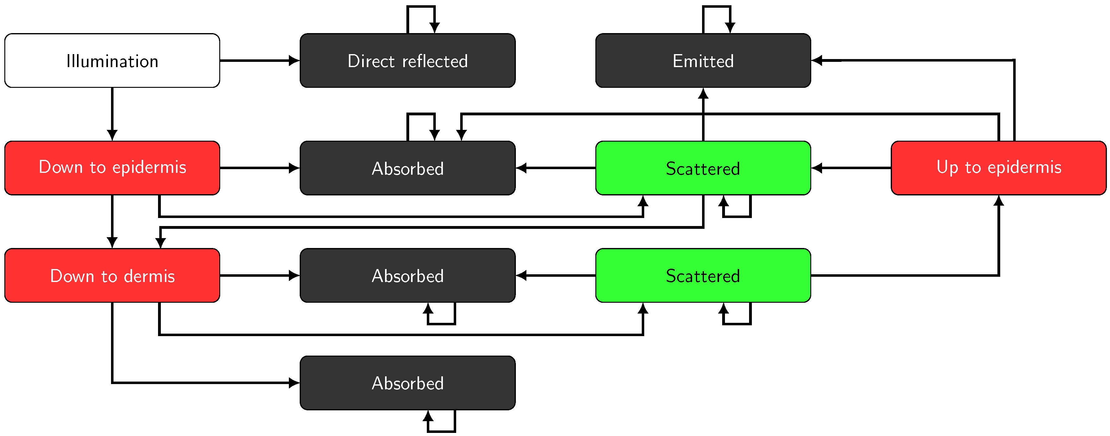
SM is the Markov chain based model for light propagation. The light propagation can be expressed as a network of transitions and states (Figure 1), in which there is a physically meaningful probability of transfer from one state to another. The probabilities are based on the chromophore concentrations and absorption and scattering properties of the skin. SM is used in the same way and with the same parameters as in [5].

In this research, the first two main skin layers, epidermis and dermis, were considered. Light through dermis was considered absorbed. From the first state, illumination, the light either goes into the skin ($P=0.98$) or is reflected ($P=0.02$). In the epidermis and dermis layers, the transition probabilities are based on Beer’s law and calculated as follows [6]:

$$\begin{array}{cc}\hfill P_{\mathrm{absorption}}\left(\lambda \right)& =\left\{\begin{array}{c}1\mathrm{if}\mathrm{the}\mathrm{current}\mathrm{state}\mathrm{is}\mathrm{absorbed},\hfill \\ \frac{a\left(\lambda \right)}{a\left(\lambda \right)+s\left(\lambda \right)}·(1-e^{-\left(a\right(\lambda )+s(\lambda \left)\right)·L})\mathrm{otherwise},\hfill \end{array}\right.\hfill \end{array}$$

(1)

$$\begin{array}{cc}\hfill P_{\mathrm{scattering}}\left(\lambda \right)& =\left\{\begin{array}{c}0\mathrm{if}\mathrm{the}\mathrm{current}\mathrm{state}\mathrm{is}\mathrm{absorbed},\hfill \\ \frac{s\left(\lambda \right)}{a\left(\lambda \right)+s\left(\lambda \right)}·(1-e^{-\left(a\right(\lambda )+s(\lambda \left)\right)·L})\mathrm{otherwise},\hfill \end{array}\right.\hfill \end{array}$$

(2)

$$\begin{array}{cc}\hfill P_{\mathrm{up}/\mathrm{down}}\left(\lambda \right)& =\left\{\begin{array}{c}1-P_{\mathrm{absorption}}-P_{\mathrm{scattering}}\mathrm{if}\mathrm{the}\mathrm{current}\mathrm{state}\mathrm{is}\mathrm{up}\mathrm{or}\mathrm{down},\hfill \\ \frac{1-P_{\mathrm{absorption}}-P_{\mathrm{scattering}}}{2}\mathrm{if}\mathrm{state}\mathrm{is}\mathrm{scattered},\hfill \\ 0\mathrm{if}\mathrm{state}\mathrm{is}\mathrm{absorbed}.\hfill \end{array}\right.\hfill \end{array}$$

(3)

In the previous equations, $\lambda$ is the wavelength in nanometers, $a\left(\lambda \right)$ is the absorption coefficient [18], and $s\left(\lambda \right)$ is the reduced scattering coefficient [18] and L is the length of the light path, which is assumed to be the same as the thickness of the layer [18].

$$\begin{array}{cc}\hfill a\left(\lambda \right)& =\sum _n{a}_i\left(\lambda \right)c_i,\mathrm{and}\hfill \end{array}$$

(4)

$$\begin{array}{cc}\hfill s\left(\lambda \right)& =s\left(500\mathrm{n}\mathrm{m}\right)·f_{\mathrm{Ray}}{\left(\frac{\lambda }{500\mathrm{n}\mathrm{m}}\right)}^{-4}+(1-f_{\mathrm{Ray}}){\left(\frac{\lambda }{500\mathrm{n}\mathrm{m}}\right)}^{-b_{\mathrm{Mie}}}\hfill \end{array}$$

(5)

In Equations (4) and (5), $a_i$ are the skin chromophore absorption coefficients and $c_i$ their concentrations, $s\left(500\mathrm{n}\mathrm{m}\right)$ the reduced scattering coefficient at $500\mathrm{n}\mathrm{m}$, $f_{Ray}$ fraction of the Rayleigh scattering and $b_{Mie}$ the Mie scattering power. The chromophores used in the study are melanin, deoxygenated and oxygenated hemoglobin and water. Their absorption coefficients are from [18], and the concentrations are in fractions of the volume they take. The deoxygenated and oxygenated hemoglobin volume fractions are calculated from blood oxygen fraction (S) and hemoglobin volume fraction ($c_{\mathrm{HGb}}$) as follows [18]:

$$\begin{array}{cc}\hfill c_{\mathrm{HGb},\mathrm{deoxy}}& =c_{\mathrm{HGb}}(1-S)\hfill \end{array}$$

(6)

$$\begin{array}{cc}\hfill c_{\mathrm{HGb},\mathrm{oxy}}& =c_{\mathrm{HGb}}S\hfill \end{array}$$

(7)

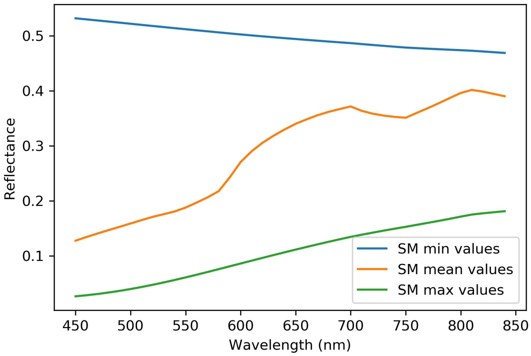
The input parameters used in SM are described in

Table 1. Input parameters and their ranges for the stochastic model. The parameters that are used as prediction targets are marked with (*). The wavelengths are described in detail in Table 2 [5].

Input Parameter	Range	Layer
* Melanosome volume fraction, $c_{\mathrm{Melanosome}}$	0–0.08	Epidermis
* Hemoglobin volume fraction, $c_{\mathrm{HGb}}$	0–0.01	Dermis
Blood oxygen saturation, S	0.2–0.5	Dermis
Water volume fraction, $c_{\mathrm{water}}$	0.5–0.8	Dermis
Reduced scattering coefficient
at 500 nm, $s\left(500\mathrm{n}\mathrm{m}\right)$	38–58	Both
Rayleigh scattering fraction, $f_{\mathrm{Ray}}$	0.38–0.42	Both
Mie scattering power, $b_{\mathrm{Mie}}$	0.3–1	Both
* Thickness of epidermis, $L_{\mathrm{epidermis}}$ (cm)	0.005–0.035	Epidermis
* Thickness of dermis, $L_{\mathrm{dermis}}$ (cm)	0.1–0.4	Dermis
Wavelength, $\lambda$ (nm)	460–843	Both

. Example spectra produced by the stochastic model are in Figure 2.

For machine learning algorithm training, the hyperspectral data simulated with SM are normalized. The prediction target parameters, melanosome, and hemoglobin volume fractions, and epidermis and dermis thicknesses, are normalized to between 0 and 1, and the spectral data are normalized to between 0 and 1 for the neural network algorithms (convolutional and regular neural networks described in Section 2.2.2 and Section 2.2.3) and to between −1 and 1 for scikit-learn algorithm implementations (other algorithms, described in Section 2.2.4–Section 2.2.6) by the StandardScaler algorithm [19].

2.1.2. Empirical Data

The empirical data were used for visual inspection of the trained machine learning regressors. The used hyperspectral image was captured using Revenio Prototype 2016 hyperspectral imager with spatial resolution of $1920\times 1200$ pixels and spectral resolution of 120 wavelengths (

Table 2. Wavelength of the measured hyperspectral data and the wavelengths used in training data production.

Wavelength (nm):	460,	461.84,	464.2,	466.43,	468.96,	471.16,	473.83,	476.66,	479.12,
	481.5,	483.88,	486.82,	489.01,	491.28,	494.12,	496.09,	498.67,	501.44,
	504.48,	506.89,	509.53,	512.15,	514.76,	517.53,	520.37,	523.1,	525.76,
	528.48,	531.25,	534.27,	536.97,	539.63,	542.39,	545.15,	547.8,	550.48,
	553.09,	555.93,	558.72,	561.27,	564.1,	566.55,	569.19,	571.85,	575.39,
	579.44,	582.22,	584.92,	587.49,	590.13,	592.77,	595.46,	598.37,	600.98,
	603.7,	606.47,	609.16,	612,	615.07,	617.84,	621.01,	623.53,	626.28,
	629.25,	632.06,	634.8,	637.95,	640.51,	643.59,	646.8,	649.04,	651.97,
	654.93,	657.75,	660.5,	663.63,	666.51,	669.53,	672.59,	675,	678.46,
	682.67,	687.25,	691.66,	696.16,	700.39,	704.64,	708.56,	712.78,	716.63,
	720.81,	725.04,	729.34,	733.99,	738.38,	742.65,	746.64,	751.27,	755.19,
	759.42,	763.86,	768.13,	772.48,	776.92,	781.83,	786.09,	790.58,	795.01,
	799.41,	803.62,	807.85,	812.18,	816.33,	820.69,	824.78,	829.33,	832.96,
	836.72,	840.25,	842.35

). The hyperspectral camera/imager is a device that captures multiple monochrome photographs in rapid succession, while controlling the wavelength of the light that gets through the controlling device to the imaging sensors. Each monochrome photograph represents a narrow wavelength interval that can be interpreted as single wavelength, such as 400 $\mathrm{n}$$\mathrm{m}$. There are usually approximately one hundred of these monochrome images in one hyperspectral image. The hyperspectral image contains the same spatial data as the normal RGB-picture, but far more data in the spectral domain, that is, the interaction between light and the subject of the image can be seen with greater precision [20].

2.2. Machine Learning Models

The inversion methods we compare are multi-layer perceptron (MLP) [21], convolutional neural network (CNN) [16], stochastic gradient descent regressor (SGD) [22], linear support vector regressor (SVR) [23], and lasso regressor [24].

The machine learning methods for inversion are selected by following criteria:

• Applicability for special characters of hyperspectral data, such as
  • nonlinearity,
  • sparsity, i.e., some wavelengths have greater significance.
• Applicability for the dataset and sample size

The multi-layer perceptron was chosen based on its applicability to nonlinear data [25,26], which is usually the case when light is scattering in complex media. The convolutional neural network fills both criteria, as it is proven to be good in image [14,15] and signal regression [16,17] problems, and it scales well to big datasets. It also takes the structure/shape of the data into account by use of convolution. The stochastic gradient descent regressor is also used in signal regression, and, according to scikit-learn documentation, version 0.23.2 [19], it is also a good fit for the size of our data, which is in the range of hundreds of thousands pixels. The lasso regressor was chosen based on the first criteria. It is also good for sparse problems [27], which means only some of the input parameters are important. This is the case with spectral data: the spectra will follow the same line in many places, but the differences are found in the wavelength zone of the chromophore of interest. The linear support vector regression was included based on its applicability on pattern recognition [28].

All machine learning algorithms were either implemented in scikit-learn Python library [19] version 0.20.1 or written by the authors using Python programming language and Tensorflow library [29] version 2.0.0.

2.2.1. Training and Testing Process

All the models were trained and tested with the simulated data. The data set consisted of 50,000 simulated spectra with associated target variables, which were melanosome volume fraction, hemoglobin volume fraction, epidermis thickness, and dermis thickness. All algorithms were trained for all targets simultaneously, resulting in regressors with an output size of four.

The data set was divided into training (n = 48,000) and test samples (n = 2000). For each method, the best set of hyperparameter values was found by the grid search method [19] and 5-fold cross-validation strategy on training samples. The final model was then trained by using all the 48,000 training samples and the best combinations of hyperparameter values. The performance of each model was then assessed with the test samples.

In addition to the simulated training and test data, empirical data were used in visual interpretation of the trained models.

2.2.2. Convolutional Neural Network

CNN is widely used in image related regression and classification tasks [14,15,16,17]. The state-of-the-art image classification algorithms utilize some form of CNN [30,31]. There is also a lot of research for it being used with hyperspectral images [10]. The CNN algorithms we used are described in

Table 3. Grid search parameters for the first convolutional neural network experiment, abbreviated as CNN in the results and discussion. The best parameters are bolded.

Parameter	Values
Convolution filters	(64 and 128), (128 and 256), (32 and 64)
Convolution kernel size	6, 9, 12
MaxPooling pool size	1, 2, 3

,

Table 4. The convolutional neural network used in first CNN inversion experiment. The best parameters from Table 3 were used.

Layer	Kernel/Pool Size	Activation	Output Shape	Parameters
Conv1D	(12)	ReLU	(109, 32)	416
MaxPooling1D	(2)		(54, 32)	0
Conv1D	(12)	ReLU	(43, 64)	24,640
MaxPooling1D	(2)		(21, 64)	0
Flatten			(1344)	0
Dense		ReLU	(128)	172,160
Dense		ReLU	(64)	8256
Dense		ReLU	(32)	2080
Dropout (0.5)			(32)	0
Dense			(4)	132
Total params:	207,684
Trainable params:	207,684
Non-trainable params:	0

,

Table 5. Grid search parameters for the second CNN experiment, abbreviated as CNNV2. The best parameters are bolded.

Parameter	Values
Amount of convolution layers	0, 3, 6
Convolution kernel size	9, 12, 15
MaxPooling pool size	1, 2, 4

and

Table 6. Convolutional neural network used in the CNNV2 experiment. The best parameters from Table 5 were used.

Layer	Kernel/Pool Size	Activation	Output Shape	Parameters
Conv1D	(15)	ReLU	(106, 64)	1020
MaxPooling1D	(2)		(53, 64)	0
Conv1D	(15)	ReLU	(39, 64)	61,504
Conv1D	(15)	ReLU	(25, 64)	61,504
MaxPooling1D	(2)		(12, 64)	0
Flatten			(768)	0
Dense		ReLU	(128)	98,432
Dense		ReLU	(64)	8256
Dense		ReLU	(32)	2080
Dropout (0.5)			(32)	0
Dense			(4)	132
Total params:	232,932
Trainable params:	232,932
Non-trainable params:	0

.

In the first experiment with grid search (Table 3), we varied the shape of two convolutional layers, the size of the convolution kernel, and size of the max-pooling [32] window. The resulting network (Table 4) had two one-dimensional, convolution layers with convolution window of size 12, 32, and 64 filters, respectively. After each convolution, there were one-dimensional, max-pooling with pool size of two. Both convolutional layers have rectified linear unit (ReLU) [33] activation. After the last max-pooling layer, there was a flattening layer and three dense layers (ReLU activation), dropout of 50%, and an output layer. The first experiment is referred to in the results and the discussion as CNN.

In the second experiment, we varied the amount of convolutional layers, the convolution kernel size, and size of the max-pooling window (Table 5). The resulting network (Table 6) consisted of a one-dimensional, convolutional neural network, max-pooling, two one-dimensional, convolution layers, another max-pooling, flattening layer three dense layers, dropout of 50% [34], and output layer. All dense and convolutional layers except output layers utilized ReLU activation. Every convolutional layer had a convolution window of size 15, and the max-pooling pool size was two. The second experiment is referred to in the results and discussion as CNNV2.

The used optimizer was an Adam optimizer [35] in both experiments. The learning rate was $0.001$, ${\beta }_1=0.9$, ${\beta }_2=0.999$ and $ϵ={10}^{-7}$, which were not included as the optimization parameters as the focus was on the architecture of the network. The loss score was mean square error (MSE).

2.2.3. Multi-Layer Perceptron

With the MLP, we varied the amount and shape of the dense layers of the network (

Table 7. Grid search parameters for MLP. The best parameters are bolded.

Parameter	Values
Dense layer shapes	(128, 64, 32), (64,32), (100,100), (200,200), (100,100,100)

). The resulting network (

Table 8. The used multi-layer perceptron. The best parameters from Table 7 were used.

Layer	Activation	Output Shape	Parameters
Flatten		(120)	0
Dense	ReLU	(100)	12,100
Dense	ReLU	(100)	10,100
Dense	ReLU	(100)	10,100
Dropout (0.5)		(100)	0
Dense		(4)	404
Total params:	32,704
Trainable params:	32,704
Non-trainable params:	0

) had a flattening input layer and three dense layers with one hundred nodes each. After the dense layers, there is a dropout of 50% and the output layer. All layers except the output layer are ReLU activated and the network optimizer is the Adam optimizer with the same parameters as CNN. The loss score was MSE.

2.2.4. Lasso

Least absolute shrinkage and selection operator (More commonly known as its acronyme: Lasso) was chosen because it works well with data where only some of the features are important [24], as is the case with our data. Mathematically, Lasso is a linear model with an added regularization term, and its objective function to minimize is

$$min\frac{1}{2n}{\left|\left|X\omega -y\right|\right|}_2^2+\alpha {\left|\left|\omega \right|\right|}_1,$$

where $\alpha$ is the penalty term, $\omega$ the fitted model, n the number of samples in the training data, X the input training data, and y the target variables. In practice, we used the MultiClassLasso algorithm from scikit-learn [19], which applies Lasso regression for all target variables at the same time.

In Lasso grid search training, we varied the $\alpha$, the stopping tolerance of the algorithm, and the selection method (

Table 9. Grid search parameters for Lasso. The best parameters are bolded.

Parameter	Values
$\alpha$	${10}^{-4},{10}^{-3}\cdots {\mathbf{10}}^{\mathbf{0}}\cdots {10}^3$
Tolerance	${10}^{-7},{10}^{-6}\cdots {\mathbf{10}}^{-\mathbf{4}}\cdots {10}^{-1}$
Selection	cyclic, random

). In the resulting estimator $\alpha =1$, $\mathrm{tolerance}={10}^{-4}$, and the selection method was cyclic.

2.2.5. Linear Support Vector Regressor

In binary classification tasks, linear support vector regressor (LSVR) means simply fitting a line or hyperplane in the space where the sum of minimum distances from each class to line is maximal. In regression, the goal is to fit a line that has the most points within a predetermined distance from the line [23].

The implementation we used was LinearSVR from scikit-learn package. It was transformed to multi-class regression by a MultiClassRegressor algorithm in scikit-learn.

With grid search (

Table 10. Grid search parameters for linear support vector machine regressor. The best parameters are bolded.

Parameter	Values
Loss	epsilon insensitive, squared epsilon insensitive
C	1, 10, 100, 1000
Dual	True, False

) for LSVR, we varied the loss method, the regularization term C, and whether or not the algorithm is solving primal or dual optimization problem.

2.2.6. Stochastic Gradient Descent Regressor

Stochastic gradient descent (SGD) is a gradient minimizing algorithm. It takes a random initial value of the input training data and tries to adjust the initial value to a point where the gradient of the objective function is zero. The adjustment is done one random observation at a time. The norm used in optimization is $L2$-norm, as opposed to $L1$-norm used in Lasso regressor [22].

The implementation we used is SGDRegressor from scikit-learn. It was transformed to multi-class regression by MultiOutputRegressor method in scikit-learn.

In grid search, we varied the regularization term $\alpha$, loss function, penalty function, and the learning rate method (

Table 11. Grid search parameters for linear stochastic gradient descent regressor. The best parameters are bolded.

Parameter	Values
Alpha	${10}^{-7},{10}^{-6}\cdots {\mathbf{10}}^{-\mathbf{4}}\cdots {10}^{-1}$
Loss	Squared loss, Huber, Epsilon insensitive
Penalty	l2, l1, elastic net
Learning rate	Constant, Optimal, Inverse scaling

). In the results and discussion, this method is referred to as a stochastic gradient descent regressor (SGDR).

2.3. Accuracy Evaluation Metrics

The following metrics were calculated from the regression results with the simulated testing data:

• Correlation coefficient (r),
• Root mean squared error (RMSE), also known as standard estimate of error (SEE),
• Mean squared error (MSE),
• Mean absolute error (MAE), and
• Saliency maps [36] were calculated only for the CNN and MLP regressors.

The correlation coefficient r was calculated to see the connection between the prediction and true target values. It is covariance (cov) of the predictions ($Y^{pred.}$) and true targets ($Y^{true}$) normalized by standard deviations ($\sigma$) for both groups:

$$r=\frac{\mathrm{cov}\left(Y^{\mathrm{pred}.},Y^{\mathrm{true}}\right)}{{\sigma }_{Y^{\mathrm{pred}.}}{\sigma }_{Y^{\mathrm{true}}}}.$$

(8)

RMSE, MSE, and MAE were calculated to capture the average errors in the predictions. They are calculated as follows:

$$\begin{array}{cc}\hfill MSE& =\frac{1}{n}\sum _{k=1}^n{(Y_k^{\mathrm{pred}.}-Y_k^{\mathrm{true}})}^2,\hfill \end{array}$$

(9)

$$\begin{array}{cc}\hfill RMSE& =\sqrt{MSE},\hfill \end{array}$$

(10)

$$\begin{array}{cc}\hfill MAE& =\frac{1}{n}\sum _{k=1}^n\left|Y_k^{\mathrm{pred}.}-Y_k^{\mathrm{true}}\right|.\hfill \end{array}$$

(11)

The saliency map shows how much each place in the map contribute to the prediction. In other words, the map indicates to which locations in the input space the output is most sensitive. The saliency map is described in detail in [36]. The saliency maps are useful in determining the most useful areas of the training data. For example, if there is need to reduce the size of the training data, one can drop the features that show lower values in the saliency map. The saliency maps were calculated using a keras-vis package version 0.4.1 [37].

3. Results

The six inversions had variable success with the simulated data (Figure 3 and Figure 4 and

Table 12. Performance metrics for the trained inversion models on the test set.

Coefficient of Correlation
	Melanosome	Hemoglobin Volume	Epidermis	Dermis
	Volume Fraction	Fraction	Thickness	Thickness
CNN	0.96	0.93	0.96	0.96
CNNV2	0.96	0.93	0.96	0.96
MLP	0.95	0.79	0.94	0.95
LASSO	0.78	0.56	0.62	0.88
LSVR	0.64	0.59	0.63	0.68
SGDR	0.78	0.55	0.62	0.88
Root Mean Squared Error
	Melanosome	Hemoglobin Volume	Epidermis	Dermis
	Volume Fraction	Fraction	Thickness	Thickness
CNN	0.10	0.12	0.09	0.10
CNNV2	0.10	0.12	0.11	0.10
MLP	0.09	0.18	0.11	0.09
LASSO	0.18	0.24	0.23	0.14
LSVR	0.23	0.24	0.23	0.22
SGDR	0.18	0.24	0.23	0.14
Mean Squared Error
	Melanosome	Hemoglobin Volume	Epidermis	Dermis
	Volume Fraction	Fraction	Thickness	Thickness
CNN	0.01	0.02	0.01	0.01
CNNV2	0.01	0.02	0.01	0.01
MLP	0.01	0.03	0.01	0.01
LASSO	0.03	0.06	0.05	0.02
LSVR	0.05	0.06	0.05	0.05
SGDR	0.03	0.06	0.05	0.02
Mean Absolute Error
	Melanosome	Hemoglobin Volume	Epidermis	Dermis
	Volume Fraction	Fraction	Thickness	Thickness
CNN	0.08	0.09	0.08	0.08
CNNV2	0.08	0.10	0.09	0.08
MLP	0.07	0.14	0.08	0.07
LASSO	0.15	0.20	0.19	0.11
LSVR	0.18	0.19	0.18	0.16
SGDR	0.15	0.20	0.18	0.11

). The CNN and CNNV2 experiments (Table 12) performed best with correlation coefficients being the highest between 0.93 and 0.96 (mean 0.95) and their RMSE, MSE, and MAE values being lowest 0.09–0.12 (mean 0.11) (RMSE), 0.01–0.02 (mean 0.01) (MSE), and 0.08–0.09 (mean 0.09) (MAE). The performance of the MLP was also good. It outscored CNN in some regression goals by some metrics and was a little poorer in others. Correlation coefficients were between 0.79 and 0.95 (mean 0.91), RMSEs 0.09–0.18 (mean 0.12), MSEs 0.01–0.03 (mean 0.02), and MAEs 0.07–0.14 (mean 0.09). Based on visual interpretation of Figure 4, the second experiment of CNN regressor is the best of the neural network regressors, as the correlation seems to be strongest there.

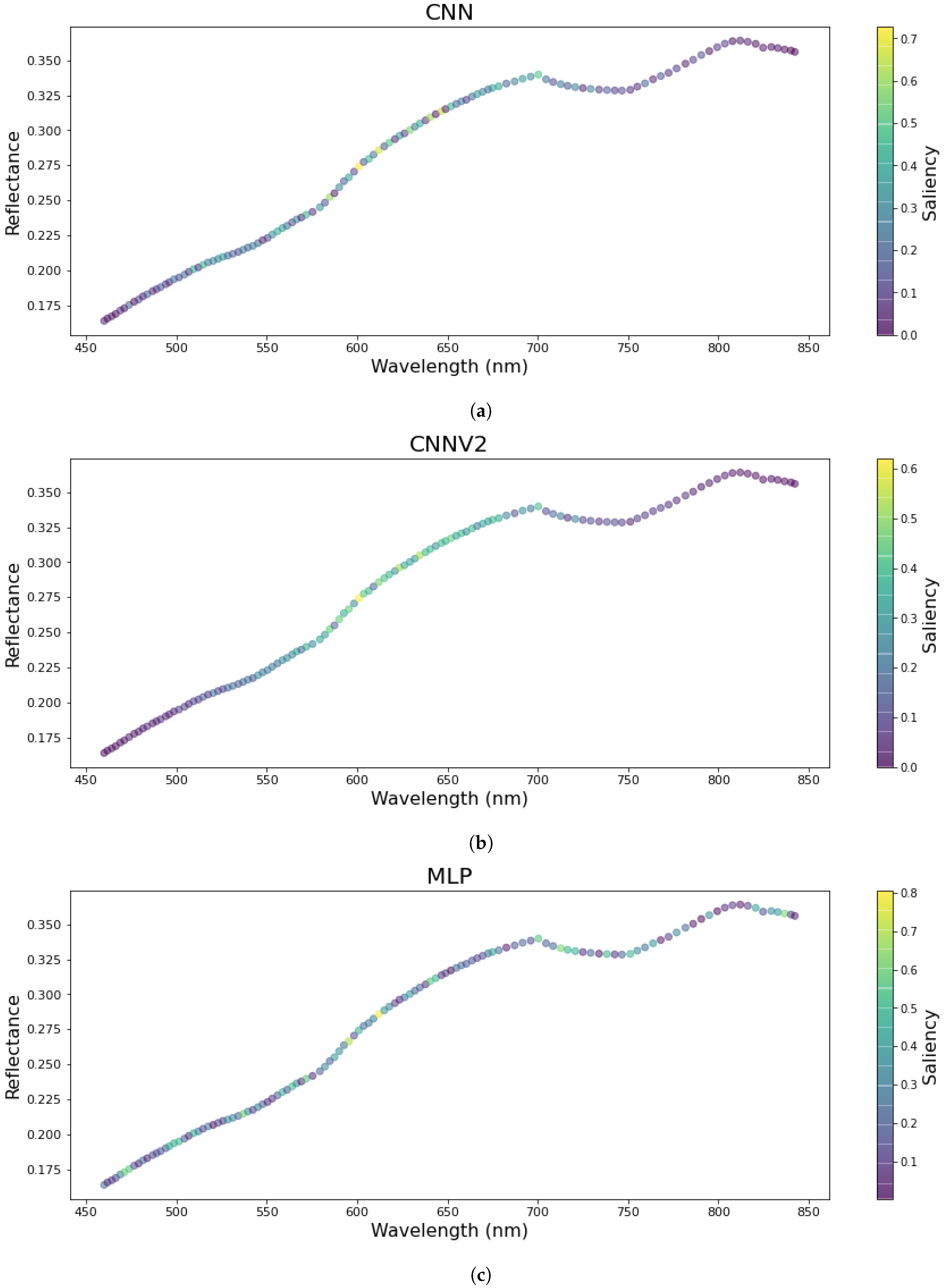
In the saliency maps of the CNN and MLP regressors (Figure 3), we see that the CNN experiments had similar areas of interest. The interval between 550 $\mathrm{n}$$\mathrm{m}$ and 700 $\mathrm{n}$$\mathrm{m}$ seems to be most important in predicting the target variables. In the MLP experiment, the same interval seems to be useful, but additionally it highlights some areas in the ends of the spectrum.

Lasso and stochastic gradient descent regressors showed similar results. As Figure 4 shows, the correlation is virtually identical, and the points scatter to nearly the same place. In fact, only looking at individual points, one can observe some differences between the lasso and SGD regressors. Lasso and SGDR had correlation coefficients between 0.55 and 0.88 (means 0.71 and 0.71, respectively), RMSEs between 0.14 and 0.24 (means 0.20 and 0.20), MSEs between 0.02 and 0.06 (means 0.04 and 0.04), and MAEs between 0.11 and 0.20 (means 0.16 and 0.16).

The worst predictor was the linear support vector regressor. It is worst by all metrics by average, but, in hemoglobin volume fraction and epidermis thickness predictions, it seems to be marginally better than Lasso and SGDR. The correlation coefficients were between 0.59 and 0.68 (mean 0.64), RMSEs between 0.22 and 0.24 (mean 0.23), MSEs between 0.05 and 0.06 (mean 0.05), and MAEs between 0.16 and 0.19 (mean 0.18).

Overall, the least accurate predictions were for hemoglobin volume fraction and the models were most accurate for dermis thickness prediction. Melanosome volume fraction was relatively easily learned by all regressors, while, in epidermis thickness, there is a clear divide between group of CNN and MLP regressors and other regressors. The neural network models provide accurate responses which seems almost impossible for the other types of models.

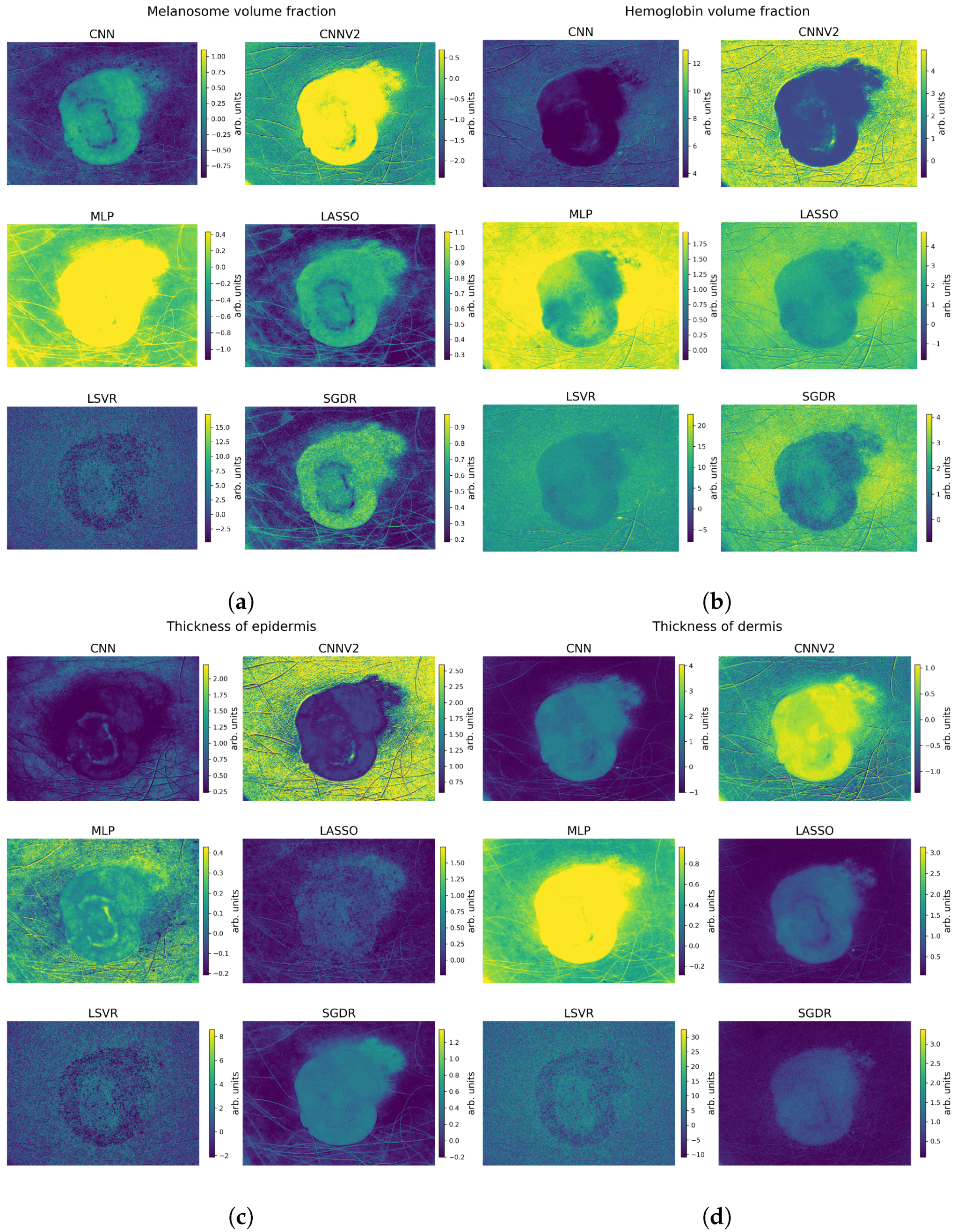
Regarding the test with the measured hyperspectral data in Figure 5, the details of the lesions are most easily visible in the CNN experiments. In MLP, lasso, and LSVR experiments, the epidermis thickness is poorly visible due to noise. Looking at Figure 5, the fourth best model seems to be the SGDR, as the details of the lesions are somewhat visible.

4. Discussion

The purpose of this study was to investigate how different machine learning approaches perform in the inversion task of predicting stochastic model parameters from the spectral input data. The present results suggests that the most accurate models can be obtained by the CNN method. It is likely that performance of all the trained models can be improved by further parameter tuning or increasing the amount of data, but it is unlikely that one model would have improvement rate vastly different from others. The results were expected as the CNN has been shown to be superior in signal processing tasks, which are essentially analogous to one-dimensional, spectral data used in this study.

The measured correlation coefficients show that the CNN is as close to perfection as can be reasonably expected without overfitting. However, we must remember that the results were achieved with simulated data, and the testing with measured biophysical parameters are yet to be carried out. The error metrics show similarly good signs, as the MAE was less than $10\%$ of the range (all true target parameters were normalized to between zero and one), and the RMSE is less than $2\%$. If the errors are similar in further testing with measured data, then the model would be ready for in-vivo clinical testing.

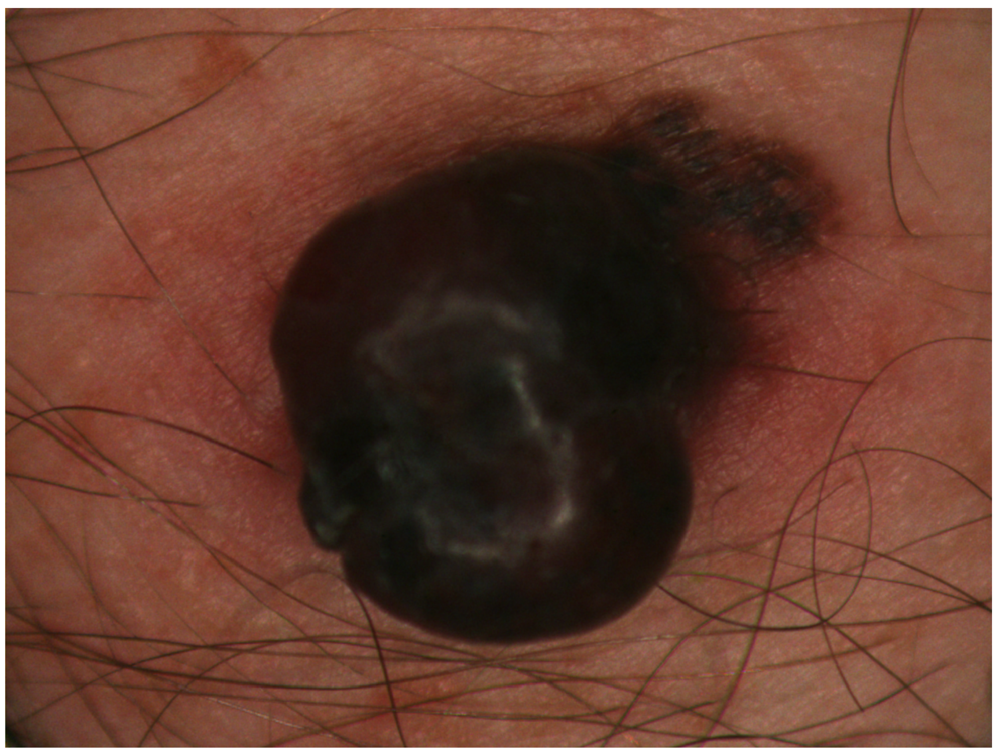
Based on the results regarding the measured hyperspectral data, it seems that the used stochastic skin model represents the optical properties of the skin quite well. The CNN predictors in Figure 5 show the same general pattern as Figure 6, and at least the melanosome volume fraction is predicted to be higher in the area of the lesion, which is clearly correct based on Figure 6. Of the absolute correctness of the model, these experiments do not provide information, as we did not have measurements of the skin biophysical parameters to compare to Figure 5.

Compared to the previous research by Vyas et al. [12,13], our correlation results are slightly inferior. They found a correlation coefficient between measured thickness and estimated thickness to be nearly perfect, while our best correlation is 0.96. However, our goal was different: we set out to find the best inversion algorithm, instead of best inversion. In future studies, we hope we can build a more robust system of parameter retrieval with a perfected CNN model.

In future research, the stochastic model and CNN combination should be thoroughly tested with measured hyperspectral data and measured biophysical parameters. The goals of the testing could include finding the best CNN estimator by optimizing the absolute and relative accuracy of the predictions with respect to the model. Our ultimate goal is to obtain a comprehensive model for predicting skin optical properties and its inverse function for predicting skin biophysical parameters.

5. Conclusions

We provided experiments that show that a convolutional neural network is a good option in skin optical model inversion and skin physical parameter retrieval. The results indicate that the most meaningful parameters of the used stochastic model were predicted accurately by the best inverted model. We also tested the inverted models while measuring the hyperspectral data, and it showed promising results to be tested in further research. It seems that the inverted model may work well with the measured data, at least when one is looking at proportional differences of skin areas instead of absolute values. Our research also suggests that the capacity of the traditional non-neural machine learning models is insufficient for accurate modeling of the hyperspectral data.

References

1. Ferlay, J.; Colombet, M.; Soerjomataram, I.; Mathers, C.; Parkin, D.; Piñeros, M.; Znaor, A.; Bray, F. Estimating the Global Cancer Incidence and Mortality in 2018: GLOBOCAN Sources and Methods. Int. J. Cancer 2019, 144, 1941–1953. [Google Scholar] [CrossRef] [PubMed] [Green Version]
2. Le, H.V.; Le, C.H.H.; Le, P.H.U.; Truong, C.T.L. Incidence and Trends of Skin Cancer in the United States, 1999–2016. J. Clin. Oncol. 2020. [Google Scholar] [CrossRef]
3. Neittaanmäki-Perttu, N.; Grönroos, M.; Jeskanen, L.; Pölönen, I.; Ranki, A.; Saksela, O.; Snellman, E. Delineating Margins of Lentigo Maligna Using a Hyperspectral Imaging System. Acta Derm. Venereol. 2015, 95, 549–552. [Google Scholar] [CrossRef] [Green Version]
4. Annala, L.; Honkavaara, E.; Tuominen, S.; Pölönen, I. Chlorophyll Concentration Retrieval by Training Convolutional Neural Network for Stochastic Model of Leaf Optical Properties (SLOP) Inversion. Remote Sens. 2020, 12, 283. [Google Scholar] [CrossRef] [Green Version]
5. Annala, L.; Pölönen, I. Kubelka-Munk Model and Stochastic Model Comparison in Skin Physical Parameter Retrieval. In Computational Sciences and Artificial Intelligence in Industry—New Digital Technologies for Solving Future Societal and Economical Challenges; Springer: Berlin/Heidelberg, Germany, 2020; in press. [Google Scholar]
6. Maier, S.W.; Lüdeker, W.; Günther, K.P. SLOP: A Revised Version of the Stochastic Model for Leaf Optical Properties. Remote Sens. Environ. 1999, 68, 273–280. [Google Scholar] [CrossRef]
7. Jolivot, R.; Benezeth, Y.; Marzani, F. Skin Parameter Map Retrieval from a Dedicated Multispectral Imaging System Applied to Dermatology/Cosmetology. J. Biomed. Imaging 2013, 2013, 978289. [Google Scholar] [CrossRef]
8. Yeh, Y.H.F.; Chung, W.C.; Liao, J.Y.; Chung, C.L.; Kuo, Y.F.; Lin, T.T. A Comparison of Machine Learning Methods on Hyperspectral Plant Disease Assessments. IFAC Proc. Vol. 2013, 46, 361–365. [Google Scholar] [CrossRef] [Green Version]
9. Sanz, J.A.; Fernandes, A.M.; Barrenechea, E.; Silva, S.; Santos, V.; Gonçalves, N.; Paternain, D.; Jurio, A.; Melo-Pinto, P. Lamb Muscle Discrimination Using Hyperspectral Imaging: Comparison of Various Machine Learning Algorithms. J. Food Eng. 2016, 174, 92–100. [Google Scholar] [CrossRef]
10. Gewali, U.B.; Monteiro, S.T.; Saber, E. Machine Learning Based Hyperspectral Image Analysis: A Survey. arXiv 2019, arXiv:1802.08701. [Google Scholar]
11. Liang, L.; Qin, Z.; Zhao, S.; Di, L.; Zhang, C.; Deng, M.; Lin, H.; Zhang, L.; Wang, L.; Liu, Z. Estimating Crop Chlorophyll Content with Hyperspectral Vegetation Indices and the Hybrid Inversion Method. Int. J. Remote Sens. 2016, 37, 2923–2949. [Google Scholar] [CrossRef]
12. Vyas, S.; Banerjee, A.; Burlina, P. Estimating Physiological Skin Parameters from Hyperspectral Signatures. J. Biomed. Opt. 2013, 18, 057008. [Google Scholar] [CrossRef] [PubMed]
13. Vyas, S.; Meyerle, J.; Burlina, P. Non-Invasive Estimation of Skin Thickness from Hyperspectral Imaging and Validation Using Echography. Comput. Biol. Med. 2015, 57, 173–181. [Google Scholar] [CrossRef] [PubMed]
14. Krizhevsky, A.; Sutskever, I.; Hinton, G.E. Imagenet Classification with Deep Convolutional Neural Networks. In Advances in Neural Information Processing Systems; ACM: New York, NY, USA, 2012; pp. 1097–1105. [Google Scholar]
15. Karpathy, A.; Toderici, G.; Shetty, S.; Leung, T.; Sukthankar, R.; Fei-Fei, L. Large-Scale Video Classification with Convolutional Neural Networks. In Proceedings of the IEEE Conference on Computer Vision and Pattern Recognition, Columbus, OH, USA, 23–28 June 2014; pp. 1725–1732. [Google Scholar]
16. LeCun, Y.; Bengio, Y. Convolutional Networks for Images, Speech, and Time-Series. In The Handbook of Brain Theory and Neural Networks; MIT Press: Cambridge, MA, USA, 1995. [Google Scholar]
17. Salamon, J.; Bello, J.P. Deep Convolutional Neural Networks and Data Augmentation for Environmental Sound Classification. IEEE Signal Process. Lett. 2017, 24, 279–283. [Google Scholar] [CrossRef]
18. Jacques, S.L. Optical Properties of Biological Tissues: A Review. Phys. Med. Biol. 2013, 58, R37. [Google Scholar] [CrossRef]
19. Pedregosa, F.; Varoquaux, G.; Gramfort, A.; Michel, V.; Thirion, B.; Grisel, O.; Blondel, M.; Prettenhofer, P.; Weiss, R.; Dubourg, V.; et al. Scikit-Learn: Machine Learning in Python. J. Mach. Learn. Res. 2011, 12, 2825–2830. [Google Scholar] [CrossRef]
20. Pölönen, I.; Rahkonen, S.; Annala, L.; Neittaanmäki, N. Convolutional Neural Networks in Skin Cancer Detection Using Spatial and Spectral Domain. In Proceedings of the SPIE BiOS, San Francisco, CA, USA, 2–7 February 2019; Volume 10851, p. 108510B. [Google Scholar]
21. Specht, D.F. A General Regression Neural Network. IEEE Trans. Neural Netw. 1991, 2, 568–576. [Google Scholar] [CrossRef] [Green Version]
22. Bottou, L. Large-Scale Machine Learning with Stochastic Gradient Descent. In Proceedings of the COMPSTAT’2010, Paris France, 22–27 August 2010; Springer: Berlin/Heidelberg, Germany, 2010; pp. 177–186. [Google Scholar]
23. Smola, A.J.; Schölkopf, B. A Tutorial on Support Vector Regression. Stat. Comput. 2004, 14, 199–222. [Google Scholar] [CrossRef] [Green Version]
24. Friedman, J.; Hastie, T.; Tibshirani, R. Regularization Paths for Generalized Linear Models via Coordinate Descent. J. Stat. Softw. 2010, 33, 1. [Google Scholar] [CrossRef] [Green Version]
25. Almeida, J.S. Predictive Non-Linear Modeling of Complex Data by Artificial Neural Networks. Curr. Opin. Biotechnol. 2002, 13, 72–76. [Google Scholar] [CrossRef]
26. Sarle, W.S. Neural Networks and Statistical Models. In Proceedings of the 19th Annual SAS Users Group International Conference, Dallas, TX, USA, 10–13 April 1994. [Google Scholar]
27. Hastie, T.; Tibshirani, R.; Friedman, J. The Elements of Statistical Learning: Data Mining, Inference, and Prediction; Springer Science & Business Media: Berlin/Heidelberg, Germany, 2009. [Google Scholar]
28. Burges, C.J. A Tutorial on Support Vector Machines for Pattern Recognition. Data Min. Knowl. Discov. 1998, 2, 121–167. [Google Scholar] [CrossRef]
29. Abadi, M.; Barham, P.; Chen, J.; Chen, Z.; Davis, A.; Dean, J.; Devin, M.; Ghemawat, S.; Irving, G.; Isard, M.; et al. Tensorflow: A System for Large-Scale Machine Learning. In Proceedings of the 12th USENIX Symposium on Operating Systems Design and Implementation (OSDI 16), Savannah, GA, USA, 2–4 November 2016; pp. 265–283. [Google Scholar]
30. Touvron, H.; Vedaldi, A.; Douze, M.; Jégou, H. Fixing the Train-Test Resolution Discrepancy: FixEfficientNet. arXiv 2020, arXiv:2003.08237. [Google Scholar]
31. Xie, Q.; Luong, M.T.; Hovy, E.; Le, Q.V. Self-Training with Noisy Student Improves Imagenet Classification. In Proceedings of the 2020 IEEE/CVF Conference on Computer Vision and Pattern Recognition, Seattle, WA, USA, 13–19 June 2020; pp. 10687–10698. [Google Scholar]
32. Scherer, D.; Müller, A.; Behnke, S. Evaluation of Pooling Operations in Convolutional Architectures for Object Recognition. In Proceedings of the International Conference on Artificial Neural Networks, Thessaloniki, Greece, 15–18 September 2010; Springer: Berlin/Heidelberg, Germany, 2010; pp. 92–101. [Google Scholar]
33. Nair, V.; Hinton, G.E. Rectified Linear Units Improve Restricted Boltzmann Machines. In Proceedings of the 27th International Conference on Machine Learning (ICML-10), Haifa, Israel, 21–24 June 2010; pp. 807–814. [Google Scholar]
34. Srivastava, N.; Hinton, G.; Krizhevsky, A.; Sutskever, I.; Salakhutdinov, R. Dropout: A Simple Way to Prevent Neural Networks from Overfitting. J. Mach. Learn. Res. 2014, 15, 1929–1958. [Google Scholar]
35. Kingma, D.P.; Ba, J. Adam: A Method for Stochastic Optimization. arXiv 2014, arXiv:1412.6980. [Google Scholar]
36. Simonyan, K.; Vedaldi, A.; Zisserman, A. Deep inside Convolutional Networks: Visualising Image Classification Models and Saliency Maps. arXiv 2013, arXiv:1312.6034. [Google Scholar]
37. Kotikalapudi, R. Keras-Vis Version 0.4.1. 2017. Available online: https://github.com/raghakot/keras-vis (accessed on 24 September 2020).
Figure 1. Network of states and transitions of light propagation in the Stochastic Model.
Applsci 10 07097 g001
Figure 2. Example spectra produced by the used stochastic model. Minimum, mean and maximum values from Table 1 were used.
Applsci 10 07097 g002
Figure 3. The saliency maps of the neural network regressors. (a) the first CNN model; (b) the second CNN model; (c) the MLP model.
Applsci 10 07097 g003
Figure 4. The scattering images of predicted values (x-axis) compared to original values (y-axis) by different regression targets: (a) melanosome volume fraction; (b) hemoglobin volume fraction; (c) thickness of epidermis; (d) thickness of dermis.
Applsci 10 07097 g004
Figure 5. Comparison of the inversion algorithms used with measured hyperspectral data. Each subfigure represents a target parameter. The colorbar units are arbitrary. (a) melanosome volume fraction; (b) hemoglobin volume fraction; (c) thickness of epidermis; (d) thickness of dermis.
Applsci 10 07097 g005
Figure 6. RGB-representation of the measured lesion.
Applsci 10 07097 g006