Optimal Neural Tracking Control with Metaheuristic Parameter Identification for Uncertain Nonlinear Systems with Disturbances

Abstract

In this paper, we propose an inverse optimal neural control strategy for uncertain nonlinear systems subject to external disturbances. This control strategy is developed based on a neural observer for the estimation of unmeasured states and inverse optimal control theory for trajectory tracking. The stabilization of states along the desired trajectory is ensured via a control Lyapunov function. The optimal parameters of the control law are identified by different nature-inspired metaheuristic algorithms, namely: Ant Lion Optimizer, Grey Wolf Optimizer, Harris Hawks Optimization, and Whale Optimization Algorithm. Finally, a highly nonlinear biological system subject to parameter uncertainties and external disturbances (Activated Sludge Model) is proposed to validate the control strategy. Simulation results demonstrate that the control law with Ant Lion Optimizer outperforms the other optimization methods in terms of trajectory tracking in the presence of disturbances. The control law with Harris Hawks Optimization shows a better convergence of the neural states in presence of parameter uncertainty.

1. Introduction

Researchers solving problems in engineering, computer science, biological, and physical sciences are developing advanced mathematical methods for control purposes. Technological advances have had a significant impact on the implementation of new analytical methods for solving nonlinear problems [1]. In most cases involving nonlinear control systems, states may not be completely measurable, which makes it difficult to solve complex control engineering problems. Other major difficulties in the area of control design are the use of a range of different models and concepts, a lack of standardization in the parameters, a lack of adequate control techniques, external disturbances, and the high level of nonlinearity of the equations that govern processes. A further issue is a lack of knowledge of important variables, since the states of the system can directly reflect the nature of the control design process allowing for high performance to be achieved [2]. It can therefore be stated that it is necessary to use advanced estimation, control, and optimization techniques to guarantee optimal nonlinear system performance. Knowledge of the system is important to understand its control requirements; however, the nonlinearities are often so complex that the control design for an adequate performance of the system is difficult [3,4,5,6]. Over time, new control strategies have emerged to ensure optimal system performance, and the estimation of states is vitally important for the development of feedback laws that allow for the avoidance of interruptions, stops, or process failures. For these reasons, it is important to develop devices called observers to estimate the missing states, and at the same time, to address the lack of online sensor measurements, the high cost of sensors, and the long laboratory analysis times [7,8]. Artificial neural networks have successfully demonstrated their feasibility and excellent performance in terms of describing highly nonlinear systems [9,10]. This is mainly due to their simplicity of deployment flexible architecture, robustness, and online learning. Several researchers have focused on the applications of neural networks applications to the identification, performance evaluation, and control of nonlinear plants [11,12]. However, most of these schemes require a complete knowledge of the variables of the mathematical model, which is not always possible. For this reason, Recurrent High Order Neural Networks (RHONN) have proven to be very useful for identification and control problems, and artificial neural networks and control strategies have been proposed to increase the system performance [13,14]. One of the main challenges in optimal control of nonlinear systems is tuning its parameters for an optimal solution. This problem has been addressed in the past by using metaheuristic techniques, since they have proved to be effective when dealing with complex systems. Metaheuristic optimization algorithms are well suited for problems with unknown search spaces, unlike deterministic algorithms. These optimization techniques find an optimal solution from a set of candidate solutions and have been used in almost every branch of science, technology, and engineering. In the last few years, a subset of metaheuristic algorithms inspired from nature, called swarm intelligence, have become more popular due to their simplicity, versatility, and flexibility [15]. Ant Lion Optimizer (ALO) has been successfully used in modeling, control, scheduling, and management with application in distributed generation, mechanics, thermal systems, and renewable energy, among others [16,17,18,19]. In [20,21], an ALO was used for parameter identification of the controller gains in a two-area thermal power system. The objective was to obtain optimal values for the control law, speed regulation, and frequency for both areas in presence of disturbances. A comparison of ALO performance with other algorithms based on standard deviations and objective functions was reported. Results showed that ALO algorithm outperforms the other optimization methods for a real problem, by obtaining precise values for the regulator design. Another nature-inspired technique, namely, Grey Wolf Optimizer (GWO) [22], has been used in [23] to control a quadrotor dynamic model and stability prediction of power systems after a large disturbance [24]. Whale Optimization Algorithm (WOA) [25] is another technique used to fine-tune neural networks to obtain more reliable models [26]. Another recently invented algorithm, Harris Hawks Optimization (HHO) [27], has been applied to optimize a controller to dampen power system oscillations [28]. Although there are many examples where these algorithms have been studied in the past, there are fewer studies that have tackled the problem of external disturbances and parameter uncertainty.

In this paper, an optimal tracking neural control strategy with metaheuristic parameter optimization is proposed for highly nonlinear, uncertain systems subject to external disturbances. In Section 2, a neural observer based on a RHONN is proposed to estimate the unmeasured states needed to develop a state feedback control law. Section 3 describes the stabilizing control law based on the inverse optimal control law theory. In Section 4, the novelty of this research is presented, the use of the newest metaheuristic algorithms, namely: ALO, GWO, HHO, and WOA for optimal parameter estimation in order to automatically find the optimal parameters of the control law. Section 5 describes the optimal control strategy architecture. To validate the efficacy of this control strategy, Section 6 presents a highly nonlinear biological system subject to disturbances as a case study. This model is applied to describe the aerobic digestion of organic matter in a continuous stirred tank reactor (CSTR). In Section 7, simulation results of the control strategy with metaheuristic algorithms are presented. Two cases are analyzed: the system subject to load disturbances and subject to uncertainties in the composition of the incoming wastewater. The total chemical oxygen demand (TCOD) is the variable of interest to be controlled by an optimal oxygen transfer (KLA) rate. Optimal operation of the wastewater treatment plant can improve energy efficiency and increase the treatment capacity. Finally, relevant conclusions are given in Section 8.

2. Neural Observer Based on RHONN

A discrete-time nonlinear system is considered as follows

$$\begin{array}{l}{z}_{k+1}=f\left(z_k\right)+g_s\left(z_k\right)u_k+d_k\\ \hspace{0.17em}{y}_k=h\left(z_k\right)\end{array}$$

(1)

where $z_k\in R^n$ is the state variable of the system at time $k\in N_{+},u_k\in R^n$ is the input control, $d_k\in R^n$ is the disturbance vector representing modeling errors and uncertain parameters, and $f\left(z_k\right)\in R^n$ and $g_s\left(z_k\right)\in R^{n\hspace{0.17em}\times \hspace{0.17em}m}$ are smooth mapping functions with $f\left(0\right)=0$ and rank$\left\{g_s\left(z_k\right)\right\}=m\hspace{0.17em},\hspace{0.17em}\forall z_k\ne 0.$ $y_k$ is the output vector and $h\left(z_k\right)\in R^{p\hspace{0.17em}\times \hspace{0.17em}n}$ is a nonlinear function of the system states.

For system (1), a RHONN is used to design a reduced order Luenberger-like observer with the following structure [29]:

$$\begin{array}{l}{\widehat{Z}}_{i,k+1}=w_{i,k}^T{\theta }_i\left({\widehat{z}}_k\right)+w^{\prime }{}_i^T{\phi }_i\left({\stackrel{⌢}{z}}_k,u_k\right)+g_i{e}_k\\ {\widehat{y}}_k=h\left({\widehat{z}}_k\right)\end{array}$$

(2)

where ${\widehat{z}}_k={\left[{\widehat{z}}_{1,k...}{\widehat{z}}_{i,k...}{\widehat{z}}_{n,k...}\right]}^T$ is the estimated state vector, $w_{i,k}\in R^n$ are the online adapted weight vectors, $w_i^{\prime T}$ is the fixed weight vector associated with the control inputs to ensure controllability of the observer, ${\phi }_i$ denotes a function of ${\widehat{z}}_k$ or $u_k$ corresponding to the plant structure (1) or external inputs to the network, respectively. $g_i\in R^p$ are the Luenberger gains, $e_k$ is the output error, and ${\theta }_i$ is an $L_P$ dimensional vector defined as

$${\theta }_i\left(z_{k,}{u}_k\right)=\left[\begin{array}{c}{\displaystyle {\prod }_{t\in I_1}{S}_{i_t}^{n_{i_t}\hspace{0.17em}(1)}}\\ {\displaystyle {\prod }_{t\in I_2}{S}_{i_t}^{n_{i_t}\hspace{0.17em}(2)}}\\ ⋮\\ {\displaystyle {\prod }_{t\in I_{L_p}}{S}_{i_t}^{n_{i_t}\hspace{0.17em}(L_p)}}\end{array}\right]$$

(3)

where $n_{i_t}$ are nonnegative integers, $L_p$ is the number of high-order connections, and $I_{L_P}$ is a collection of nonordered subsets of $\left\{1,2,\dots ,n+m\right\}.$ S_i is a sigmoid function vector defined as:

$$s\left(z_k\right)=\frac{{\alpha }_i}{\hspace{0.17em}1\hspace{0.17em}+\hspace{0.17em}{e}^{-\beta i}};\hspace{0.17em}{\alpha }_i,{\beta }_i>0$$

(4)

The output error is defined by:

$$e_k=y_k-{\stackrel{⌢}{y}}_k.$$

(5)

The output error can be minimized by an appropriate selection of $L_p$. $w_i^{*}$ and $w^{\prime *}$ are assumed ideal weight matrices for analytical purposes, and these are constant but unknown. The optimal unknown weights $w_{i.k}^{*}$ are approximated by online adjustable versions $w_{i,k}$.

For online learning of the RHONN weights, an Extended Kalman Filter (EKF) is used [30]. EKF training of recurrent neural networks has proven its applicability to extensive difficult modeling and control problems. The sequential nature of the EKF provides a stochastic component that allows for more effective search of the weight space. The EKF methods are easily implemented in software and hardware. Perhaps the most significant limitation of EKF training is its limited applicability to cost functions other than minimizing sum of squared error. For the proposed neural network training, the cost function criterion is satisfied. The weights of the neural network become the estimated states. The neural network training to find the optimal weight values is as follows:

$$\begin{array}{l}{w}_{i,k+1}=w_{i,k}+{\eta }_i{K}_{i,k}{e}_k{}_{,}\\ K_{i,k}=P_{i,k}{H}_{i,k}{M}_{i,k}\\ P_{{}_{i,k+1}=}{P}_{i,k}-K_{i,k}{H}_{i,k}^T{P}_{i,k}{Q}_{i,k}\\ M_{i,k}={\left[R_{i,k}+H_{i,k}^T{P}_{i,k}{H}_{i,k}\right]}^{-1}\end{array}$$

(6)

where $w_{i,k}\in R^{Li}$ is the weight vector, ${\eta }_i$ is the learning rate, $K_{i,k}\in R^{Li\times p}$ is the Kalman gain matrix, $P_{i,k}\in R^{Li\times li}$ is the prediction error associated covariance matrix, $Q_{i,k}\in R^{Li\times li}$ is the state noise associated covariance matrix, $M_{i,k}\in R^{p\times p}$ is a global scaling matrix, $R_{i,k}\in R^{p\times p}$ is the measurement noise associated covariance matrix, and $H_{i,k}\in R^{Li\times n}$ is a matrix of the derivatives of the network outputs with respect to all trainable neural network weights as follows:

$$H_{i,k}=\left[\frac{\partial {\widehat{y}}_k}{\partial w_{i,k}}\right]$$

(7)

$L_i$ is the total number of neural network weights. $P_i$, $Q_i$, and $R_i$ are initialized as diagonal matrices. During training, $K_{i,k}$, $P_{i,k}$, and $H_{i,k}$ are ensured to be bounded [31].

3. Discrete-Time Inverse Optimal Control

Consider the following cost function related to trajectory tracking of the nonlinear system in (1)

$$J\left({\delta }_k\right)={\displaystyle \sum _{n=k}^{\infty }\left(l\left({\delta }_n\right)+u_n^T{R}_z{u}_n\right)}$$

(8)

where $\delta =z_k-z_{r,k}$; $z_{r,k}$ is the desired trajectory for $z_k$, $J\left({\delta }_k\right):R^n\to R^{+};\hspace{0.17em}l\left({\delta }_k\right):R^n\to R^{+}$ is a positive semidefinite function, and $R_z:R^n\to R^{+}$ is a real weighting matrix, symmetric and positive definite for control efforts. The cost function in (8) is a performance measurement. Availability of system states is necessary for the state feedback control design. Using the optimal value function $J^{\ast }\left({\delta }_k\right)$ for (8) as a Lyapunov function $V_L\left({\delta }_k\right)$, the cost function can be rewritten as [32]

$$\begin{array}{ll}{V}_L\left({\delta }_k\right)& =l\left({\delta }_k\right)+u_k^T{R}_z{u}_k+{\displaystyle \sum _{n=k+1}^{\infty }l\left({\delta }_n\right)}+u_k^T{R}_z{u}_k\\ \hspace{0.17em}& =l\left({\delta }_k\right)+u_k^T{R}_z{u}_k+V_L\left({\delta }_{k+1}\right)\end{array}$$

(9)

From Bellman’s principle of optimality [33], for the case of infinite time horizon optimization, the value function $V_L^{*}\left({\delta }_k\right)$ becomes time invariant and satisfies the discrete-time Bellman equation. The boundary condition V(0) = 0 must be satisfied so that $V_L\left({\delta }_k\right)$ becomes a Lyapunov function. The following discrete-time Hamiltonian [32] is defined

$$H\left({\delta }_k,u_k\right)=l\left({\delta }_k\right)+u_k^T{R}_z{u}_k+V_L\left({\delta }_{k+1}\right)-V_L\left({\delta }_{k+1}\right)-V_L\left({\delta }_k\right)$$

(10)

A necessary condition for the optimal control law $u_k$ is $\partial H\left({\delta }_k,u_k\right)/\partial u_k=0$. Then,

$$0=2R{u}_k+\frac{\partial V_L\left({\delta }_{k+1}\right)}{\partial u_k}=2R{u}_k+g_s^T\left(z_k\right)\frac{\partial V_L\left({\delta }_{k+1}\right)}{\partial {\delta }_k}$$

(11)

The optimal control law to achieve trajectory tracking is therefore formulated as follows

$$u_k^{*}=\frac{1}{2}{R}^{-1}{g}_s^T\left(z_k\right)\frac{\partial V_L\left({\delta }_{k+1}\right)}{\partial {\delta }_{k+1}}$$

(12)

By substituting (12) in (10), the Hamilton–Jacobi–Bellman (HJB) equation is obtained. Solving this equation is a challenging task, and to address this problem, inverse optimal control based on Lyapunov stability is proposed [32].

Definition: Tracking Inverse Optimal Control

For the control law in (12) and tracking error ${\delta }_k=z_k-z_{r,k}$, inverse optimal stabilization along the desired trajectory is guaranteed if:

(i)

(global) asymptotic stability of $z_k$ along reference $z_{r,k}$ is achieved

(ii)

$V_L\left({\delta }_k\right)$ is a (radially unbounded) positive definite function and satisfies the inequality

$$\overline{V}\left({\delta }_k\right):V_L\left({\delta }_{k+1}\right)-V_L\left({\delta }_k\right)+u_k^T{}^{*}{R}_z{u}_k^{*}\le 0$$

(13)

The inverse optimal control law for trajectory tracking is based on a knowledge of $V_L\left({\delta }_k\right)$, and a Control Lyapunov Function (CLF) $V_L\left({\delta }_k\right)$ is proposed to ensure that requirements (i) and (ii) are satisfied. Hence, instead of solving the HJB equation for $V_L\left({\delta }_k\right)$ a CLF is proposed as follows:

$$V_L\left({\delta }_k\right)=\frac{1}{2}{\delta }_k^T{P}_L{\delta }_k,\hspace{0.17em}{P}_L=P^T>0$$

(14)

By substituting (14) in (12), the following control law is obtained:

$$u_k^{*}=\frac{1}{2}{\left[R_z+\frac{1}{2}{g}_s^T\left(z_k\right)P_L{g}_s\left(z_k\right)\right]}^{-1}\hspace{0.17em}{g}_s^T\left(z_k\right)P_L\left(f\left(z_k\right)-z_{r,k+1}\right)$$

(15)

where P_L and R_Z are positive definite symmetric matrices that guarantee the existence of the inverse function in (15). The proof that the control law in (15) ensures stability and optimality for (1) is given in [32].

4. Metaheuristic Optimization Algorithms

In this section, the four optimization algorithms used in this paper are briefly described. It is worth noting that the versions used are the original proposed by their respective author, thus variants, hybrids, or improved versions are not considered.

4.1. Ant Lion Optimizer

The main inspiration for the ALO algorithm was the foraging behavior of antlion larvae [16]. The algorithm mimics the interactions between antlions and their prey (ants) in traps. To model these interactions, ants move around the search space and antlions try to hunt them and become more sophisticated at using traps. Because the movements of ants when searching for food are stochastic in nature, a random walk or move is chosen to model this movement, as follows:

$$X(t)=\left[0,cumsum\left(2r\left(t_1\right)-1\right),cumsum\left(2r\left(t_2\right)-1\right),....,cumsum\left(2r\left(t_n\right)-1\right)\right]$$

(16)

where cumsum computes the cumulative sum, n represents the number of iterations, t is the step of the random walk (or iteration), and r(t) is a function that is defined as follows:

$$\begin{array}{l}r\left(t\right)=\{\begin{array}{c}\hspace{0.17em}\hspace{0.17em}\hspace{0.17em}1\hspace{0.17em}\hspace{0.17em}\hspace{0.17em}if\hspace{0.17em}\hspace{0.17em}\hspace{0.17em}rand\hspace{0.17em}>\hspace{0.17em}0.5\\ \hspace{0.17em}\hspace{0.17em}\hspace{0.17em}0\hspace{0.17em}\hspace{0.17em}\hspace{0.17em}if\hspace{0.17em}\hspace{0.17em}\hspace{0.17em}rand\hspace{0.17em}\le \hspace{0.17em}0.5\end{array}\\ \end{array}$$

(17)

where t is the step of the random walk and rand is a random number produced with a uniform distribution on the interval [0, 1].

The random moves are based on Equation (17). Ants update their position with a random move at every step of the process. Given that every search space has a boundary, Equation (16) is not directly used to update the position of an ant. In order to keep the random moves inside the search space, they need to be normalized using the following equation, which is a min–max normalization:

$$X_i^t=\frac{\left(X_i^t-a_i\right)\times \left(d_i-c_i^t\right)+c_i}{\left(b_i^t-a_i\right)}$$

(18)

where $a_i$ is the minimum random move for the ith variable, $b_i^{}$ is the maximum random move for the ith variable, $c_i^t$ is the minimum for the ith variable at the ith iteration, and $d_i^t$ is the maximum for the ith variable at the ith iteration. Equation (18) should be applied at each iteration to ensure that random moves are confined to the search space.

When the prey is close to the trap, antlions hurl grains of sand outwards from the pit, causing the ant to slide further down. This behavior is modeled by reducing the radius of the ants’ random walk using the following equations:

$$c^t=\frac{c^t}{I},d^t=\frac{d^t}{I}$$

(19)

where I is a ratio, $c_{}^t$ is the minimum of all the variables in the ith iteration and $d_{}^t$ is a vector that includes the maximum of all variables in the ith iteration.

When an ant falls to the bottom of the pit, the antlion updates its position to the last position of the ant in order to increase the chances of catching the prey. For this, the following equation is used:

$$Antlio{n}_j^t=An{t}_i^t,if(An{t}_i^t)>f(Antlio{n}_j^t)$$

(20)

where t is the current iteration, $Antlio{n}_j^t$ is the position of the chosen jth antlion at tth iteration, and $An{t}_i^t$ is the position of the ith ant at tth iteration.

At the end, the fittest antlion for each iteration is kept and considered elite. Given that the elite is the best antlion, it affects the movements of all the ants during the iterations. Thus, every ant walks randomly around a selected antlion by means of a roulette wheel and the elite as follows:

$$An{t}_i^t=\frac{R_A^t+R_E^t}{2}$$

(21)

where $R_A^t$ is the random move around the selected antlion by the roulette wheel at the tth iteration, $R_E^t$ is the random move around the elite at the tth iteration, and $An{t}_i^t$ is the position of the tth ant at the tth iteration. Figure 1 shows the pseudo code for the ALO algorithm.

4.2. Grey Wolf Optimizer

The Grey Wolf Optimizer is inspired in the collective behavior of a pack of wolves hunting together [23]. Grey wolves show a very well-defined social hierarchy, where the leader of the pack is called dominant or alpha (α). The alpha wolf is in charge of making decisions about moving from one area to another, when to sleep, hunt, etc. The next level in their hierarchy is the beta wolf (β), which is the group of wolves that help the alpha to discipline the pack. The beta wolf is normally the best candidate to lead the pack when the alpha dies or becomes too old. The next level is the delta wolf (δ) and they serve as scouts or sentinels. Lastly, the omega wolf (ω) is the lowest in rank, it serves as the scapegoat and they are the last ones to eat. The omega wolves are actually very useful to the pack, since without them the pack would fight with each other.

Grey wolves work as a team and their hunting strategy is described in three steps: Finding and chasing the prey, surrounding and frightening until it stops moving, and attack. In the GWO algorithm, the search for pray corresponds to the exploration of the space and the attacking step to the exploitation phase. The encircling behavior is governed by the following equations:

$$D=\left|C\cdot X_p(t)-X(t)\right|$$

(22)

$$X(t+1)=X_p(t)-A\cdot D$$

(23)

where t is the current iteration, X_p is a vector that represents the position of the prey, A and C are coefficient vectors, and X the position of a grey wolf.

Vectors A and C are obtained as follows:

$$A=2a\cdot r_1-a$$

(24)

$$C=2\cdot r_2$$

(25)

where r₁ and r₂ are random vectors in [0, 1] and a is a vector with components that decrease linearly from 2 to 0 during iterations.

The alpha wolf usually leads the hunt and the beta and delta join. However, in an optimization search space, the location of the best position is not known; therefore, the GWO algorithm assumes that these wolves are closer to the location of the prey. Their three positions are saved, and the rest of the pack is encouraged to follow them updating their positions according to the following formulas:

$$D_{\alpha }=\left|C_1\cdot X_{\alpha }-X\right|,D_{\beta }=\left|C_2\cdot X_{\beta }-X\right|,D_{\delta }=\left|C_3\cdot X_{\delta }-X\right|$$

(26)

$$X_1=X_{\alpha }-A_1\cdot (D_{\alpha }),X_2=X_{\beta }-A_2\cdot (D_{\beta }),X_2=X_{\delta }-A_3\cdot (D_{\delta })$$

(27)

$$X(t+1)=\frac{X_1+X_2+X_3}{3}$$

(28)

The pseudo code in Figure 2 describes the GWO algorithm:

4.3. Harris Hawks Optimization

The Harris Hawks Optimization relatively new algorithm proposed by Heidari et al. [27] in 2019. It is a nature-inspired population-based technique that mimics the cooperative behavior and hunting style of Harris’ hawks. These raptors pounce a prey from different angles, attempting to surprise it and they display different chasing patterns depending on the particular natural scenarios and escaping patterns of the pray (usually rabbits). The HHO algorithm, as many of the other nature-inspired techniques, has both exploration and exploitation phases. For the exploration phase, they have mainly two strategies: one of them consists in perching based on the locations of other hawks, in order to be close to them at the moment of the attack, and the second strategy is perching based on random tall trees, still close to other members. Both strategies are equally probable and denoted by q in Equation (29), which models this behavior:

$$X\left(t+1\right)=\{\begin{array}{c}\hspace{0.17em}{X}_{rand}(t)-r_1\left|X_{rand}(t)-2r_{2}X(t)\right|\hspace{0.17em}\hspace{0.17em}\hspace{0.17em}if\hspace{0.17em}\hspace{0.17em}q\hspace{0.17em}\ge \hspace{0.17em}0.5\\ \hspace{0.17em}(X_{rabbit}(t)-X_m(t))-r_3(LB+r_4(UB-LB))\hspace{0.17em}\hspace{0.17em}\hspace{0.17em}if\hspace{0.17em}\hspace{0.17em}q\hspace{0.17em}<\hspace{0.17em}0.5\end{array}$$

(29)

where $X\left(t+1\right)$ is the position vector of the hawks for the next iteration t. $X_{rabbit}$ is the position of the rabbit, $X\left(t\right)$ is the current position of the hawks, r₁, r₂, r₃, r₄, and q are random numbers in the range of (0, 1) and are updated in each iteration, LB and UB are the upper and lower bounds of variables, $X_{rand}\left(t\right)$ is a hawk selected randomly from the current population, and $X_m$ is the average position of the current population of hawks.

The HHO algorithm transfers from exploration to exploitation and changes between different exploitative strategies based on the energy of the prey. This energy decreases during the escaping behavior, which is modeled by the following equation:

$$E=2E_0(1-\frac{t}{T})$$

(30)

where E is the escaping energy of the rabbit, T is the maximum number of iterations, and E₀ is the initial state of the energy. E₀ randomly changes in the interval (−1, 1) at each iteration. When its value decreases from 0 to −1, the prey is physically weak, and when it increases from 0 to 1, the prey strengthens. The dynamic escaping energy E decreases during the iterations.

The next phase is called “soft besiege” when the rabbit still has energy and tries to escape performing random misleading jumps. This behavior is modeled by the following rules:

$$X(t+1)=\Delta X(t)-E\left|J{X}_{rabbit}(t)-X(t)\right|$$

(31)

$$\Delta X(t)=X_{rabbit}(t)-X(t)$$

(32)

where $\Delta X(t)$ is the difference between the position vector of the prey and the current location at iteration t, $J=2(1-r_5)$ represents the random hop strength of the rabbit when trying to escape, and r₅ is a random number in (0, 1). The value of J changes to simulate the random movement of the rabbit.

“Hard besiege” is when the prey is very tired and has low escaping energy. The Harris’s hawks surround the prey to finally execute the surprise pounce. Their current positions are updated by Equation (33):

$$X(t+1)=X_{rabbit}(t)-E\left|\Delta X(t)\right|$$

(33)

The pseudo code for the HHO algorithm is described in Figure 3.

4.4. Whale Optimization Algorithm

The Whale Optimization Algorithm is inspired by the foraging behavior of humpback whales [25]. These mammals have a complex social behavior, which helps them to hunt in groups to feed on their favorite prey: krill. Humpback whales hunt krill and small fishes that swim close to the surface. They create distinctive bubbles along a circle path around the school, creating what is called a bubble-net to trap their prey.

Because the solution of an optimization problem on the search space is not known, the whale optimization algorithm assumes that the optimal candidate is the target prey. The behavior of the whales or search agents is given by the following equations:

$$D=\left|C{X}^{*}(t)-X(t)\right|$$

(34)

$$X(t+1)=X^{*}(t)-A\cdot D$$

(35)

where t indicates the current iteration, X is the position vector, A and C are coefficient vectors, and X* is the position vector of the best solution so far. X* is to be updated in each iteration when a better solution is found. The vectors A and C are determined as follows:

$$A=2a\cdot r-a,C=2r$$

(36)

where a linearly decreases from 2 to 0 during iterations and r is a random vector in [0, 1].

The exploitation phase is called “Bubble-net attacking” where the whales circle their prey performing a spiral shape, which is described by the following equation:

$$X(t+1)=D^{\prime }\cdot e^{bl}\cdot \cos (2\pi l)+X^{*}(t)$$

(37)

where $D^{\prime }=\left|X^{*}(t)-X(t)\right|$ is the distance of the ith whale to the prey, b is a constant to define the shape of the logarithmic spiral, and l is a random number in [−1, 1].

The exploration phase consists of a random search by each whale with A ≥ 1 or A ≤ 1, where A is a random value in order to force each whale to move away from a reference whale. The mathematical model is as follows:

$$D=\left|C\cdot X_{rand}-X\right|$$

(38)

$$X(t+1)=X_{rand}-A\cdot D$$

(39)

where $X_{rand}$ is a random position vector chosen from the current population. The pseudo code for the WOA algorithm is shown in Figure 4.

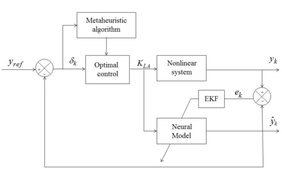
5. Optimal Control Strategy Architecture

Nonlinear systems can have a complex dynamic behavior based on the stability of their equilibrium points. Convergence of nonlinear system states to one operating point can be unpredictable depending on the nature and the initial state of the system, such that robust control strategies are necessary. Figure 5 displays the optimal neural control strategy for uncertain nonlinear systems subject to disturbances. The RHONO estimates unmeasured states of the nonlinear system needed to develop a state feedback control law. The controlled system could work properly in the presence of small disturbances but, for large disturbances and parameter uncertainties, the system could be unstable affecting the performance and operating safety. In order to address this issue, metaheuristic algorithms are used to identify optimal tuning parameters for controller. The metaheuristic algorithms propose a P_L matrix for the CLF to reduce the mean square tracking error between the neural model state and its given trajectory reference. Optimization strategy stops when the reference trajectory is reached, and the CLF matrix satisfice the asymptotic stability condition given in Section 3. The optimization strategy is able to find optimal parameters for reference trajectories tracking of different operating points.

6. Case Study

The mathematical model is derived from Activated Sludge Model No. 1 (ASM1) [34] and describes the aerobic digestion process that occurs in a CSTR, consisting of the material balances of the components, the kinetics, and the stoichiometry of the major processes in the plant. The TCOD is the variable of interest that will be controlled by regulating the KLA. The following nonlinear discrete-time Equations (40)–(49) describe the biological transformation processes that occur in the reactor, and Figure 6 illustrates the plant configuration.

Readily biodegradable soluble substrate

$$X_{1,k+1}=D\left(X_{1,in}-X_{1,k}\right)-\frac{1}{YH}.{\mu }_{\max ,H}.{\mu }_1.({\mu }_3+{\mu }_6.{\mu }_4.n_g)X_{3,k}+k_h.{\mu }_7\left({\mu }_3+n_h.{\mu }_6.{\mu }_4\right)X_{3,k}$$

(40)

Slowly biodegradable particulate substrate

$$X_{2,k+1}=D\left(X_{2,in}-X_{2,k}\right)+D_r(b-1)X_{2,k}+(1-fp)(b_H{X}_{3,k}+b_A{X}_{4,k})-k_h.{\mu }_7({\mu }_3+n_h.{\mu }_6.{\mu }_4)X_{3,k}$$

(41)

Active heterotrophic particulate biomass

$$X_{3,k+1}=D\left(X_{3,in}-X_{3,k}\right)+D_r\left(b-1\right)X_{3,k}+{\mu }_{\max ,H}.{\mu }_1.{\mu }_3.X_{3,k}+{\mu }_{\max ,H}.{\mu }_1.{\mu }_6.{\mu }_4.ng.X_{3,k}-b_H.X_{3,k}$$

(42)

Active autotrophic particulate biomass

$$X_{4,k+1}=D\left(X_{4,in}-X_{4,k}\right)+D_r\left(b-1\right)X_{4,k}+{\mu }_{\max ,A}.{\mu }_5.{\mu }_2.X_{4,k}-b_A.X_{4,k}$$

(43)

Soluble oxygen

$$X_{5,k+1}=D\left(X_{5,in}-X_{5,k}\right)+KLA\left(X_{5,\max }-X_5\right)-\frac{\left(1-Y_H\right)}{Y_H}.{\mu }_{\max ,H}.{\mu }_1.{\mu }_3.X_{3,k}-\frac{\left(4.57-Y_A\right)}{Y_A}.{\mu }_{\max ,A}.{\mu }_5.{\mu }_2.X_{4,k}$$

(44)

Soluble nitrate and nitrite nitrogen

$$X_{6,k+1}=D\left(X_{6,in}-X_{6,k}\right)-\frac{\left(1-Y_H\right)}{2.86Y_H}.{\mu }_{\max ,H}.{\mu }_1.{\mu }_6.{\mu }_4.n_g.X_3+\frac{1}{Y_A}.{\mu }_{\max ,A}.{\mu }_5.{\mu }_2.X_4$$

(45)

Soluble ammonium (NH+ 4 and NH) nitrogen

$$X_{7,k+1}=D\left(X_{7,in}-X_{7,k}\right)-i_{XB}{\mu }_{\max ,H}.{\mu }_1\left({\mu }_3+{\mu }_6.{\mu }_4.n_g\right)X_3-\left(i_{XB}+\frac{1}{Y_A}\right){\mu }_{\max ,A}.{\mu }_5.{\mu }_2.X_{4,k}+k_A.X_{8,k}.X_{3,k}$$

(46)

Soluble biodegradable organic nitrogen

$$X_{8,k+1}=D\left(X_{8,in}-X_{8,k}\right)-k_A.X_{8,k,}.X_{3,k}+k_h.{\mu }_7\left({\mu }_3+n_h{\mu }_6{\mu }_4\right)X_{3,k}\frac{X_{9,k}}{X_{2,k}}$$

(47)

Particulate biodegradable organic nitrogen

$$\begin{array}{ll}{X}_{9,k+1}=& D\left(X_{9,in}-X_{9,k}\right)+D_r\left(b-1\right)X_{9,k}+\left(i_{XB}-f_p.i_{XP}\right)\left(b_H.X_{3,k}+b_A.X_{4,k}\right)\\ \hspace{0.17em}& -k_h.k_{sat}.\left({\mu }_3+n_h.{\mu }_6.{\mu }_4\right)X_{3,k}.\frac{X_{9,k}}{X_{2,k}}\end{array}$$

(48)

Parameters of the model and Monod reaction rates ${\mu }_i,\hspace{0.17em}i=1,...,7$ [35] are given in Appendix A. The inputs of the plant are the dilution rates (D, D_r), KLA, biomass, and substrate concentrations (X_i,in). The output of the plant is the TCOD given by (49), which is composed of the readily biodegradable soluble substrate (X_1,k), the slowly biodegradable particulate substrate (X_2,k), and the inert soluble and particulate organic material (I_s). The steady-state value for I_s is given by the corresponding constant value of the influent:

$$TCOD=X_{1,k}+X_{2,k}+I_s$$

(49)

7. Results

The performance of the control strategy for trajectory tracking is verified with the biological nonlinear model (40)–(49), in the presence of load disturbances and parameter uncertainty. Reference trajectories are proposed based on the hydraulic retention time (HRT) of the wastewater treatment plant, and the maximal daily rate of organic biodegradability per biomass unit. Neural network structure for the biological model consists of five neurons in the hidden layer and one neuron at the output layer, with a logistic and a linear activation function, respectively. The neural network estimates the X_1,k and X_2,k states of the system in order to calculate the TCOD output. Parameter of the neural structure are given in Appendix A. The optimization consists of using each of the metaheuristic algorithms (ALO, GWO, HHO, and WOA) to find the best set of parameters to configure the control law (15) for optimal trajectory tracking. In order to configure the control law, matrix P_L is used as the variable to be optimized. P_L is a symmetric matrix, where all values must be real positive numbers. Because the matrix is symmetric, values P_L12 and P_L21 are the same, thus the vector to be optimized consists of three variables: [P_L11, P_L12, P_L23]. The fitness function is the mean square tracking error between the neural model state and its given trajectory reference; thus, the objective is to minimize the area between desired trajectory and the actual output. In this section, two cases are presented where tracking error is compared when the system is subject to load disturbances and parameter uncertainty, respectively. In the following tests, the metaheuristic algorithms were configured as follows: 50 search agents, 100 iterations, a lower boundary of 0.00001, and an upper boundary of 1. MATLAB R2016a (Mathworks Inc., Natick, MA, USA) was used for these mathematical simulations.

7.1. External Disturbance

In all of the case studies, reference paths are used to comply with the TCOD requirements. The allowable TCOD concentration leaving a wastewater treatment plant has a maximum value of 50 mg COD/L. A step disturbance with an amplitude equal to 40% of the steady-state value X_1in (the input concentration of readily biodegradable substrate) is applied at t = 5 d. The tracking error comparison is displayed in Figure 7 and Figure 8.

Figure 7 displays the tracking error for substrates along their respective desired trajectories. For the case of the neural model control with ALO algorithm, the tracking performance for both substrates is better than the other methods. For both sceneries, the neural model presents a slightly transient state error when disturbance is applied at t = 5 days. Figure 8a shows the TCOD tracking error as function of the substrates defined by (49). As in the previous test, the TCOD with ALO algorithm presents a good convergence along the desired trajectory as compared with the other methods. Figure 8b portrays the KLA signal behavior to reach the reference trajectories of the system. A time variant behavior of KLA is observed before the disturbance is applied, and then the KLA signal shows an incremental response over the remaining simulation time to reject the disturbance. For the case of the neural model control with ALO algorithm, the KLA signal illustrates a stable increasing behavior over the simulation time up to a value of 5 d⁻¹, maintaining the system along the reference trajectories. Thus, the control law with ALO outperforms the other methods in terms of tracking trajectory in a nonlinear disturbed system.

7.2. Parameter Uncertainty

Active heterotrophs are known to govern TCOD removal in activated sludge systems, and the biodegradation rates are expressed in terms of the active biomass. In this test, the biodegradation rate is investigated by increasing the maximum specific growth rate ${\mu }_{\max ,H}$ by 20% for active heterotrophic biomass at t = 5 d. Figure 9 and Figure 10 illustrate the tracking error comparison in the presence of parameter uncertainty.

Figure 9 illustrates the tracking error performance for the substrates in the presence of parameter uncertainty. The neural model control using metaheuristic algorithms shows a good tracking performance with a neglected transient state error. For this test, HHO shows a better convergence along the trajectory reference in presence of parameter uncertainty. Figure 10a shows the TCOD tracking error as a result of the transient error of the substrates. Figure 10b displays the KLA signal behavior to reach reference trajectories of the system. The KLA shows a time variant behavior after the parameter uncertainty. For the case of the control law with WOA algorithm, KLA shows an increasing stable performance over simulation time up to a value of 4.8 d⁻¹ to reject the disturbance. Thus, the control strategy with WOA demonstrates a more stable behavior for KLA, but control law with HHO shows a better convergence for the neural states. Thus, the control law combined with these metaheuristic algorithms is effective in terms of tracking trajectory in presence of parameter uncertainty.

8. Conclusions

This paper proposes an optimal neural tracking control strategy for nonlinear uncertain systems subject to external disturbances. The novelty of this strategy is the use of the newest metaheuristic algorithm (ALO, GWO, HHO, and WOA) implementation to find optimal tuning of the control law. Efficacy of the coupled strategy is proven in a highly nonlinear biological model subject to disturbances, uncertainties, and hard to measure state variables. A neural observer based on a RHONN is proposed to estimate the unmeasured states of the system necessary to develop a state feedback control law. Inverse optimal control theory for trajectory tracking based on a neural model is used to design a stabilizing control law. In order to evaluate the efficiency of the coupled strategy, four configurations with metaheuristic algorithms are used. Two case studies are examined, system subject to load disturbances, and parameter uncertainty, respectively. Results via simulations show that the optimal control law combined with the ALO metaheuristic algorithm is a robust method of stabilizing the system states along the reference trajectories in presence of external disturbances. Optimal control law combined with the HHO is effective in presence of parameter uncertainty. Control strategy with the other methods shows a significant transient state error due to a limited tuning. Thus, optimal operation of the plant can improve energy efficiency and increase the treatment capacity. As future work, the control strategy will be proven in a real scale pilot plant for wastewater treatment to validate its efficacy.

References

1. Kumar, A.; Jain, T. Sub-optimal Control Design for Second Order Non-linear Systems using Krotov Sufficient Conditions. IFAC Pap. 2020, 53, 272–276. [Google Scholar] [CrossRef]
2. Yu, Q.; Hou, Z.; Bu, X.; Yang, J. Observer-based data-driven constrained norm optimal iterative learning control for unknown non-affine non-linear systems with both available and unavailable system states. J. Frankl. Inst. 2020, 357, 5852–5877. [Google Scholar] [CrossRef]
3. Ballesteros, M.; Chairez, I.; Poznyak, A. Robust optimal feedback control design for uncertain systems based on artificial neural network approximation of the Bellman’s value function. Neurocomputing 2020, 413, 134–144. [Google Scholar] [CrossRef]
4. Wu, X.; Shen, J.; Wang, M.; Lee, K.Y. Intelligent predictive control of large-scale solvent-based CO2 capture plant using artificial neural network and particle swarm optimization. Energy 2020, 196, 117070. [Google Scholar] [CrossRef]
5. Gurubel, K.J.; Sanchez, E.N.; Coronado-Mendoza, A.; Zuniga-Grajeda, V.; Sulbaran-Rangel, B.; Breton-Deval, L. Inverse optimal neural control via passivity approach for nonlinear anaerobic bioprocesses with biofuels production. Optim. Contr. Appl. Methods 2019, 40, 848–858. [Google Scholar] [CrossRef]
6. Mcclamroch, N.H.; Kolmanovsky, I. Performance benefits of hybrid control design for linear and nonlinear systems. Proc. IEEE 2000, 88, 1083–1096. [Google Scholar] [CrossRef]
7. Gurubel, K.J.; Sanchez, E.N.; González, R.; Coss y León, H.; Recio, R. Artificial Neural Networks Based on Nonlinear Bioprocess Models for Predicting Wastewater Organic Compounds and Biofuel Production. In Artificial Neural Networks for Engineering Applications; Academic Press: St. Louis, MI, USA, 2019; pp. 79–96. [Google Scholar] [CrossRef]
8. Alanis, A.Y.; Sanchez, E.N. Discrete-Time Neural Observers: Analysis and Applications; Academic Press: London, UK, 2017. [Google Scholar]
9. Alanis, A.Y.; Sanchez, E.N.; Loukianov, A.G.; Hernandez, E.A. Discrete-time recurrent high order neural networks for nonlinear identification. J. Frankl. Inst. 2010, 347, 1253–1265. [Google Scholar] [CrossRef]
10. Siregar, S.P.; Wanto, A. Analysis of Artificial Neural Network Accuracy Using Backpropagation Algorithm In Predicting Process (Forecasting). Int. J. Inf. Syst. Technol. 2017, 1, 34–42. [Google Scholar] [CrossRef] [Green Version]
11. Pisa, I.; Morell, A.; Vicario, J.L.; Vilanova, R. Denoising Autoencoders and LSTM-Based Artificial Neural Networks Data Processing for Its Application to Internal Model Control in Industrial Environments-the Wastewater Treatment Plant Control Case. Sensors 2020, 20, 3743. [Google Scholar] [CrossRef]
12. Schmitt, F.; Banu, R.; Yeom, L.-T.; Do, K.-U. Development of artificial neural networks to predict membrane fouling in an anoxic-aerobic membrane bioreactor treating domestic wastewater. Biochem. Eng. J. 2018, 133, 47–58. [Google Scholar] [CrossRef]
13. Sadeghassadi, M.; Macnab, C.J.B.; Gopaluni, B.; Westwick, D. Application of neural networks for optimal-setpoint design and MPC control in biological wastewater treatment. Comput. Chem. Eng. 2018, 115, 150–160. [Google Scholar] [CrossRef]
14. Leon, B.S.; Alanis, A.Y.; Sanchez, E.N.; Ornelas-Tellez, F.; Ruiz-Velazquez, E. Neural Inverse Optimal Control via Passivity for Subcutaneous Blood Glucose Regulation in Type 1 Diabetes Mellitus Patients. Intell. Autom. Soft. Comput. 2014, 20, 279–295. [Google Scholar] [CrossRef]
15. Mirjalili, S.; Dong, J.S.; Lewis, A. Nature-Inspired Optimizers: Theories, Literature Reviews and Applications; Springer: Cham, Switzerland, 2019; Volume 811. [Google Scholar] [CrossRef]
16. Heidari, A.A.; Faris, H.; Mirjalili, S.; Aljarah, I.; Mafarja, M. Ant lion optimizer: Theory, literature review, and application in multi-layer perceptron neural networks. In Nature-Inspired Optimizers; Springer: Cham, Switzerland, 2020; pp. 23–46. [Google Scholar] [CrossRef]
17. Fathy, A.; Kassem, A.M. Antlion optimizer-ANFIS load frequency control for multi-interconnected plants comprising photovoltaic and wind turbine. ISA Trans. 2019, 87, 282–296. [Google Scholar] [CrossRef]
18. Pradhan, R.; Majhi, S.K.; Pradhan, J.K.; Pati, B.B. Antlion optimizer tuned PID controller based on Bode ideal transfer function for automobile cruise control system. J. Ind. Inf. Integr. 2018, 9, 45–52. [Google Scholar] [CrossRef]
19. Verma, S.; Mukherjee, V. Optimal real power rescheduling of generators for congestion management using a novel ant lion optimiser. IET Gener. Transm. Dis. 2016, 10, 2548–2561. [Google Scholar] [CrossRef]
20. Gupta, E.; Saxena, A. Performance evaluation of antlion optimizer based regulator in automatic generation control of interconnected power system. J. Eng. 2016. [Google Scholar] [CrossRef] [Green Version]
21. Saikia, L.C.; Sinha, N. Automatic generation control of a multi-area system using ant lion optimizer algorithm based PID plus second order derivative controller. Int. J. Electr. Power. 2016, 80, 52–63. [Google Scholar] [CrossRef]
22. Mirjalili, S.; Mirjalili, S.M.; Lewis, A. Grey Wolf Optimizer. Adv. Eng. Softw. 2014, 69, 46–61. [Google Scholar] [CrossRef] [Green Version]
23. Oliveira, J.; Oliveira, P.M.; Boaventura-Cunha, J.; Pinho, T. Evaluation of Hunting-Based Optimizers for a Quadrotor Sliding Mode Flight Controller. Robotics 2020, 9, 22. [Google Scholar] [CrossRef] [Green Version]
24. Arefi, M.; Chowdhury, B. Post-fault transient stability status prediction using Grey Wolf and Particle Swarm Optimization. In Proceedings of the SoutheastCon 2017, Charlotte, NC, USA, 30 March–2 April 2017; pp. 1–8. [Google Scholar] [CrossRef]
25. Mirjalili, S.; Lewis, A. The Whale Optimization Algorithm. Adv. Eng. Softw. 2016, 95, 51–67. [Google Scholar] [CrossRef]
26. Tien Bui, D.; Abdullahi, M.M.; Ghareh, S. Fine-tuning of neural computing using whale optimization algorithm for predicting compressive strength of concrete. Eng. Comput. 2019. [Google Scholar] [CrossRef]
27. Heidari, A.A.; Mirjalili, S.; Faris, H.; Aljarah, I.; Mafarja, M.; Chen, H. Harris hawks optimization: Algorithm and applications. Future Generat. Comput. Syst. 2019, 97, 849–872. [Google Scholar] [CrossRef]
28. Devarapalli, R.; Bhattacharyya, B. Application of Modified Harris Hawks Optimization in Power System Oscillations Damping Controller Design. In Proceedings of the 8th International Conference on Power Systems (ICPS), Jaipur, India, 20–22 December 2019; pp. 1–6. [Google Scholar] [CrossRef]
29. Alanis, A.Y.; Sanchez, E.N.; Ricalde, L.J. Discrete-time reduced order neural observers for uncertain nonlinear systems. Int. J. Neural Syst. 2010, 20, 29–38. [Google Scholar] [CrossRef] [PubMed] [Green Version]
30. Haykin, S. Kalman Filtering and Neural Networks; John Wiley & Sons: New York, NY, USA, 2004; Volume 47. [Google Scholar]
31. Sanchez, E.N.; Alanís, A.Y.; Loukianov, A.G. Discrete-Time High Order Neural Control Trained with Kalman Filtering; Springer: Berlin, Germany, 2008. [Google Scholar]
32. Sanchez, E.N.; Ornelas-Tellez, F. Discrete-Time Inverse Optimal Control for Nonlinear Systems; CRC Press: Boca Raton, FL, USA, 2017. [Google Scholar]
33. Wang, D.; Liu, D.; Wei, Q.; Zhao, D.; Jin, N. Optimal control of unknown nonaffine nonlinear discrete-time systems based on adaptive dynamic programming. Automatica 2012, 48, 1825–1832. [Google Scholar] [CrossRef]
34. Henze, M.; Gujer, W.; Mino, T.; van Loosdrecht, M.C. Activated Sludge Models ASM1, ASM2, ASM2d and ASM3; IWA Publishing: London, UK, 2000. [Google Scholar]
35. Nelson, M.I.; Sidhu, H.S. Analysis of the activated sludge model (number 1). Appl. Math. Lett. 2009, 22, 629–635. [Google Scholar] [CrossRef] [Green Version]
Figure 1. Pseudo code of the Ant Lion Optimizer algorithm.
Applsci 10 07073 g001
Figure 2. Pseudo code of the Grey Wolf Optimizer algorithm.
Applsci 10 07073 g002
Figure 3. Pseudo code of the Harris Hawks Optimization algorithm.
Applsci 10 07073 g003
Figure 4. Pseudo code of the Whale Optimization Algorithm algorithm.
Applsci 10 07073 g004
Figure 5. Optimal neural tracking control strategy for nonlinear systems.
Applsci 10 07073 g005
Figure 6. Wastewater plant configuration.
Applsci 10 07073 g006
Figure 7. Tracking performance comparison in presence of external disturbance: (a) X1,k and (b) X2,k.
Applsci 10 07073 g007
Figure 8. Tracking performance comparison in presence of external disturbance: (a) TCOD control and (b) KLA signal.
Applsci 10 07073 g008
Figure 9. Tracking performance comparison in presence of parameter uncertainty: (a) X1,k and (b) X2,k.
Applsci 10 07073 g009
Figure 10. Tracking performance comparison in presence of parameter uncertainty: (a) TCOD control and (b) KLA signal.
Applsci 10 07073 g010