Energy Performance Forecasting of Residential Buildings Using Fuzzy Approaches

Abstract

The energy consumption used for domestic purposes in Europe is, to a considerable extent, due to heating and cooling. This energy is produced mostly by burning fossil fuels, which has a high negative environmental impact. The characteristics of a building are an important factor to determine the necessities of heating and cooling loads. Therefore, the study of the relevant characteristics of the buildings, regarding the heating and cooling needed to maintain comfortable indoor air conditions, could be very useful in order to design and construct energy-efficient buildings. In previous studies, different machine-learning approaches have been used to predict heating and cooling loads from the set of variables: relative compactness, surface area, wall area, roof area, overall height, orientation, glazing area and glazing area distribution. However, none of these methods are based on fuzzy logic. In this research, we study two fuzzy logic approaches, i.e., fuzzy inductive reasoning (FIR) and adaptive neuro fuzzy inference system (ANFIS), to deal with the same problem. Fuzzy approaches obtain very good results, outperforming all the methods described in previous studies except one. In this work, we also study the feature selection process of FIR methodology as a pre-processing tool to select the more relevant variables before the use of any predictive modelling methodology. It is proven that FIR feature selection provides interesting insights into the main building variables causally related to heating and cooling loads. This allows better decision making and design strategies, since accurate cooling and heating load estimations and correct identification of parameters that affect building energy demands are of high importance to optimize building designs and equipment specifications.

1. Introduction

In recent years there has been a substantial increase of research in the area of energy performance in buildings. The aim is to design and construct more energy-efficient buildings in order to reduce their energy consumption and CO2 emissions. Buildings are responsible for approximately 40% of energy consumption and 36% of CO2 emissions in the EU, making them the single largest energy consumer in Europe. Residential buildings comprise the biggest segment of the EU’s building stock and are responsible for the majority of the sector’s energy consumption [1]. The European Commission (EC) boosted the research in this area with a program framed in Horizon 2020 [1]. In the Energy Efficiency Plan in Europe, the EC states that a greatest energy saving potential lies in buildings. The minimum energy savings in buildings can generate a reduction of 60–80 Mtoe in final energy consumption by 2020, and make a considerable contribution to the reduction of greenhouse gas (GHG) emissions [2].

Machine-learning (ML) strategies, within the field of artificial intelligence, have already been used to deal with estimation and performance of energy consumption in buildings, as summarized in the recent review by Seyedzadeh et al. [3]. The main ML techniques widely used in the energy building sector are artificial neural network (ANN) and support vector machines (SVM). ANN models have been applied mainly for fast estimation of heating and cooling loads [4], energy consumption and efficiency [5,6] and optimization and control of heating systems [7,8]. In the building sector, SVM have been mainly used for classification of energy usage [9], cooling and heating loads forecasting [10] and prediction of energy consumption [11]. Other ML and soft computing techniques, as for example genetic algorithms (GA) or random forest (RF), have also been used in this area to a lesser extent [12,13]. Contrarily, up to our knowledge, Fuzzy logic based methods have been applied sparingly to the energy performance estimation of buildings.

Fuzzy logic approaches, within the analysis of energy in buildings, have been used mainly in the control area [14] and in multiple criteria decision-making [15]. However, up to our knowledge, Fuzzy logic based methods have been applied sparingly to the energy performance estimation of buildings.

In this research we propose to apply fuzzy logic modelling for energy performance forecasting of residential buildings. In the building energy field, the use of fuzzy logic modelling approaches can be a very good alternative due to its potentiality to work with uncertainties, to explain effectively complex relationships and to understand uncertain causal relations between variables. In addition, its capacity to obtain high accuracy predictions is of great importance when dealing with energy consumption. These reasons encourage us to make an exploration of non-linear fuzzy approaches, i.e., fuzzy inductive reasoning (FIR) and adaptive neuro fuzzy inference system (ANFIS), for estimating energy performance of residential buildings. A first attempt in this direction has been presented in reference [16].

Tsanas and Xifara [17] generated a set of simulated residential buildings that are available in the UCI machine-learning repository [18]. It is important to remark that the use of simulated building data is useful and justified when dealing with energy prediction challenges, since it allows researchers to reduce considerably the time needed to obtain the data, design easily different building configurations and work with a lower level of detail. As claimed by the authors, the data generated represent with high probability actual real data, enabling energy comparisons between buildings.

In their research, classical linear regression and random forest approaches were used to predict the heating and cooling load of residential buildings [17]. Other studies used additional ML approaches, i.e., neural networks, support vector machines, evolutionary computation, etc., to deal with the same problem and working with the same data set [19,20,21].

The first goal of this paper, is to compare the performance of fuzzy approaches (FIR and ANFIS) with respect to 13 predictive modelling methodologies, from the prediction capability point of view. The study of the performance of fuzzy approaches is a novelty in respect of heating and cooling load prediction from building design characteristics, since none of the previous studies have worked with this kind of system. The second goal of this research is to study the feature selection capability of the FIR methodology to determine the relevance of each of the variables involved in the study from the prediction point of view. The reduced set of features selected by FIR are used as inputs to ANFIS models, showing that the level of prediction accuracy is not reduced but the computational time is decreased substantially. This is the first time that FIR is proposed as a feature selection pre-process for other modelling methodologies, as for example ANFIS.

The structure of the paper is organized as follows: Section 2 introduces the FIR and ANFIS methodologies. In Section 3, FIR and ANFIS models are identified with the goal of energy performance forecasting of residential buildings. Section 4 presents a discussion of the results obtained by the fuzzy approaches and the FIR feature selection process, and performs an analysis of its usefulness. In Section 5, the main conclusions are offered.

2. Fuzzy Methodologies

Both FIR and ANFIS machine-learning approaches proposed in this research are hybrid methodologies that combine mainly soft computing techniques. FIR combines fuzzy logic with k-nearest neighbours while ANFIS combines fuzzy logic with neural networks.

FIR and ANFIS, as fuzzy methodologies, have some main differences that are listed below:

-

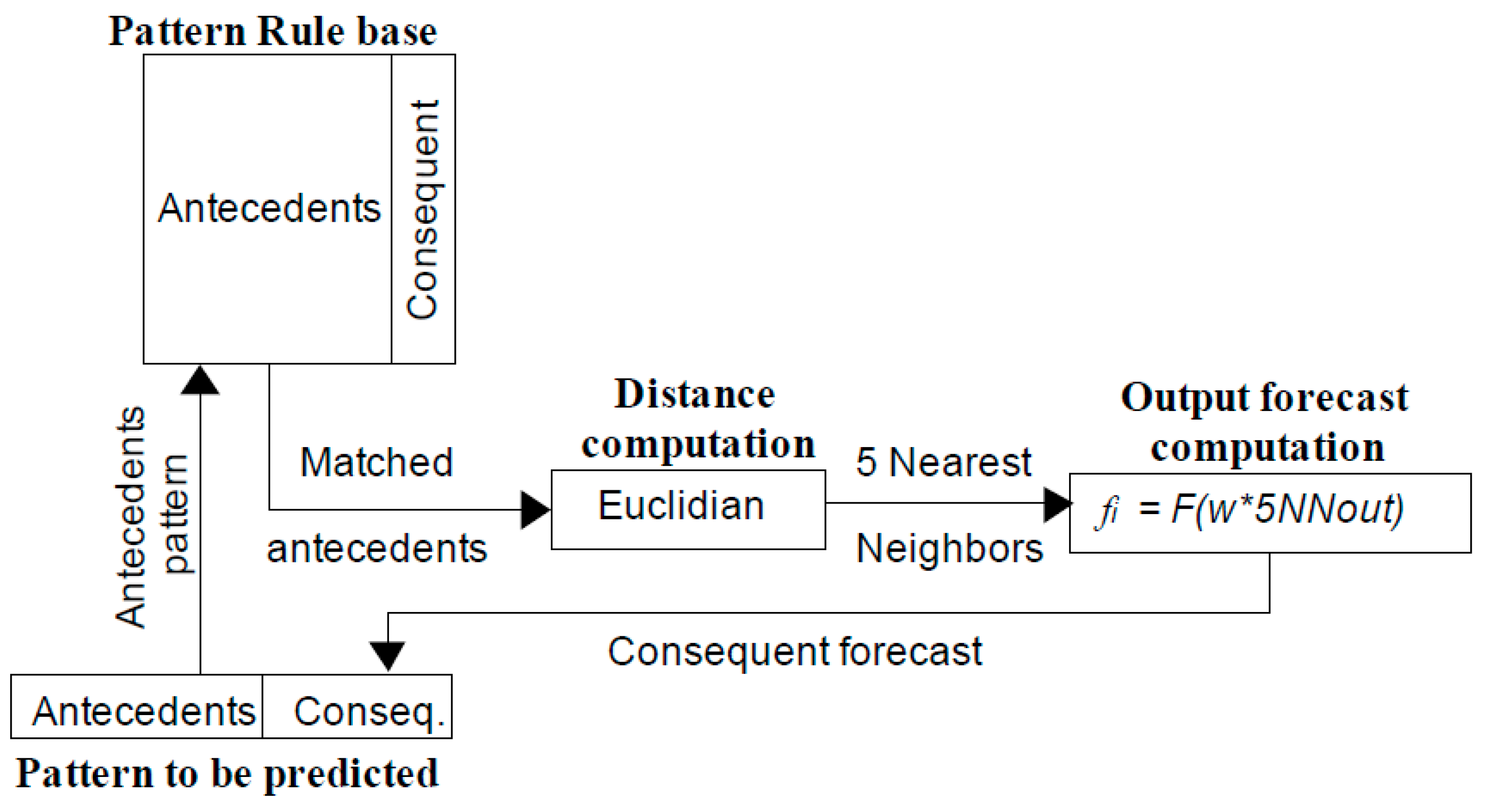
ANFIS is a pure fuzzy inference system, i.e., a fuzzy system is trained and a fuzzy inference process is performed for prediction. FIR identifies a fuzzy model that represents the system under study, but the prediction is performed applying a k-nearest neighbour (KNN) hybrid approach.

-

ANFIS models are trained by means of neural network training algorithms. FIR models are synthesized rather than trained, meaning that an optimization process is performed to organize the training data appropriately.

-

ANFIS models are Sugeno-type fuzzy systems where the antecedents are fuzzy sets and the consequent is not a fuzzy set, but a function. FIR, on the contrary, uses fuzzy sets to represent both the antecedents and the consequent, being more useful for obtaining explainable models that can be used for decision making.

-

FIR has an internal feature selection (FS) process that allows identifying the input variables that are most relevant in the inference process and their degree of individual relevance. ANFIS has no FS integrated in its structure, and it is necessary to apply a FS algorithm as a pre-process, if desired.

The main characteristics of these two methodologies are summarized in this section.

2.1. Fuzzy Inductive Reasoning (FIR)

The conceptualization of the FIR methodology arises from the General System Problem Solving (GSPS) approach proposed by Klir [22]. FIR offers a model-based approach to predicting either univariate or multi-variate time series [23,24,25,26]. Visual-FIR is a tool based on the FIR methodology (runs under Matlab environment), that offers a new perspective on the modelling and simulation of complex systems.

FIR is composed of four main processes: fuzzification, qualitative model identification, fuzzy forecasting, and defuzzification. The fuzzification process converts quantitative data stemming from the system into fuzzy data. The qualitative model identification process is responsible for finding causal and temporal relations between variables (feature selection process) and is used to obtain the best model that represents the system. Once the FIR model is available, the prediction system can take place using the FIR inference engine. This process is called fuzzy forecasting. The FIR inference engine is a specialization of the KNN algorithm, commonly used in the pattern recognition field. Defuzzification is the inverse process of fuzzification, it allows converting the qualitative predicted output into quantitative values that can then be used as inputs to an external quantitative model.

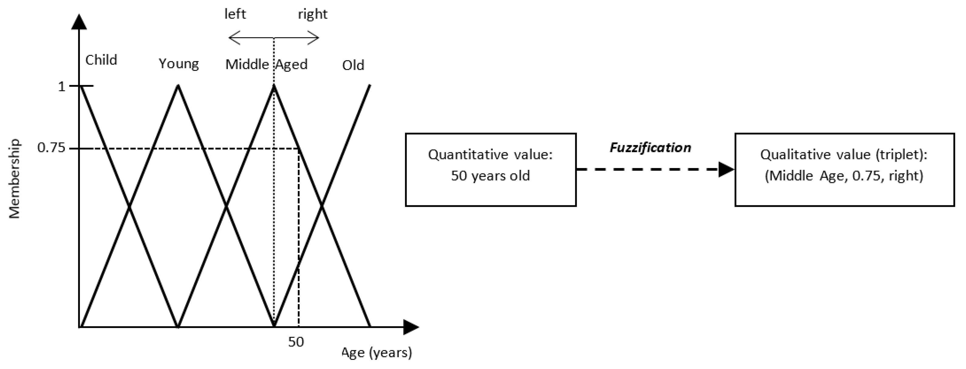
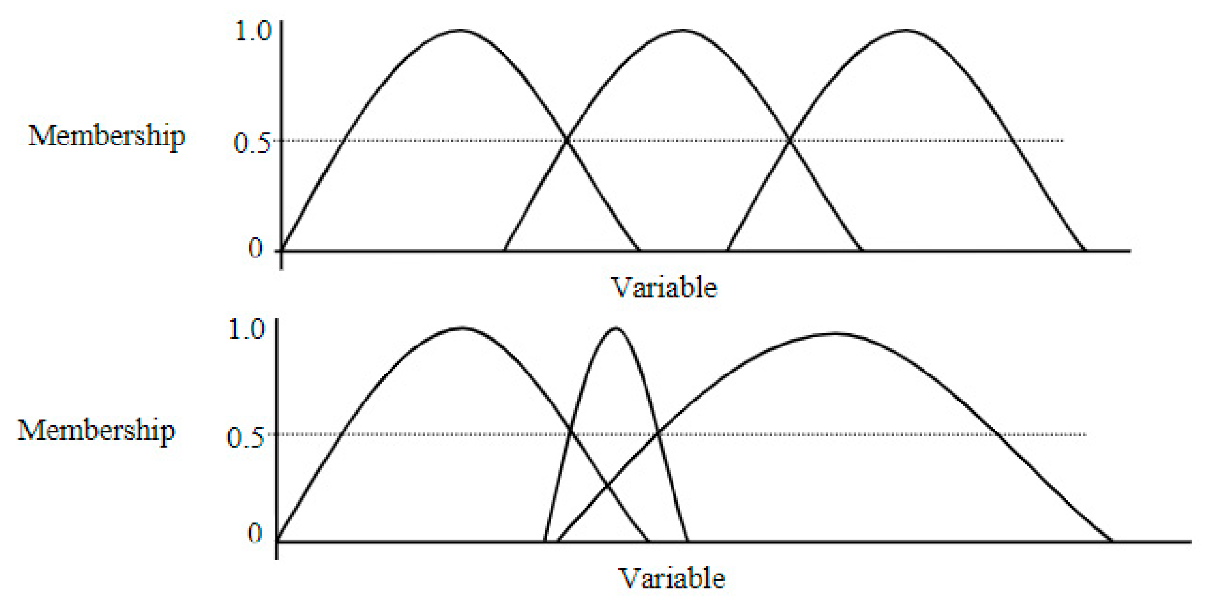
2.1.1. Fuzzification

Figure 1 illustrates the process of fuzzification by means of an example.

A quantitative value is fuzzified into a qualitative triple. The first element of the triple is the class value, the second element is the fuzzy membership value, and the third element is the side value. The side value indicates whether the qualitative value is to the left or right of the peak value of the associated membership function. The side value is responsible for preserving, in the qualitative triple, the complete knowledge that had been contained in the original quantitative value. According to Figure 1, a human age of 50 years old would be fuzzified into the class Middle Age (class where a value of 50 years has the highest membership value), a fuzzy membership value of 0.75 and a side value of right (because 50 years is to the right hand side of the maximum membership value of the class Middle Age).

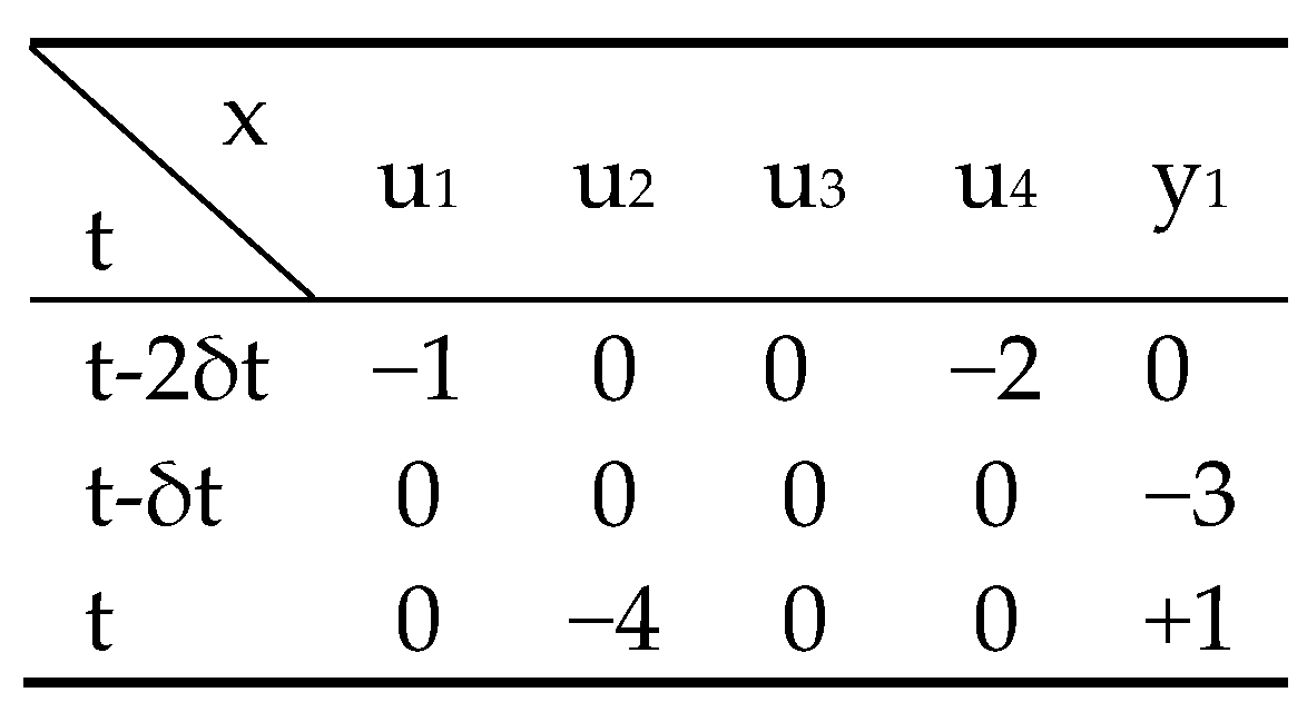
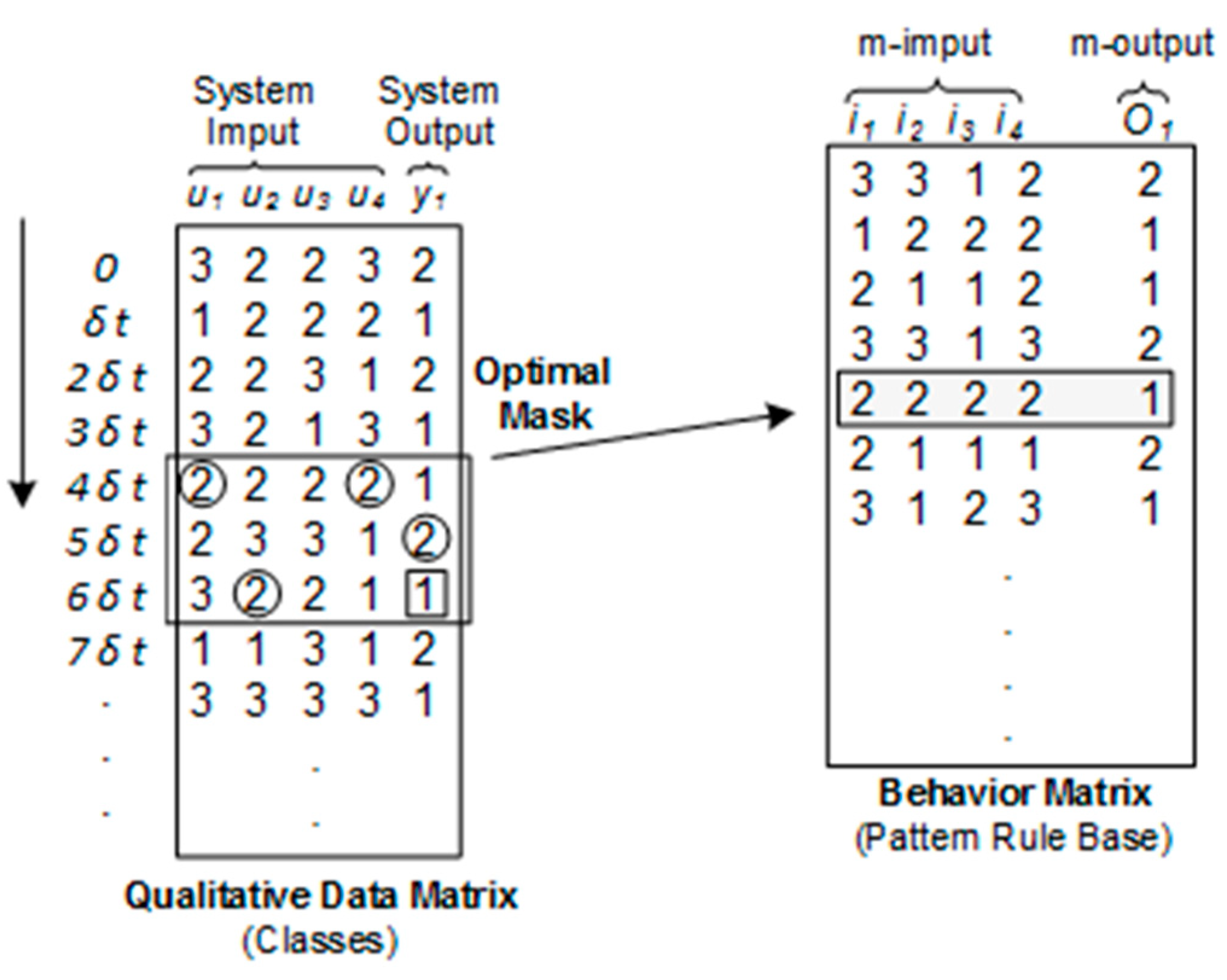
2.1.2. Qualitative Model Identification

A FIR model is composed by a structure, called mask, and a pattern rule base, named behaviour matrix. A mask denotes a dynamic relationship among qualitative variables. An example of a mask is presented in Figure 2.

Each negative element in the mask is called m-input (mask input). It denotes a causal relation with the output, that is, it influences the output up to a certain degree. The enumeration of the m-inputs is immaterial and has no relevance. The single positive value denotes the m-output. The mask of Figure 2 contains four m-inputs. In this example, the first and second m-inputs, i₁ and i₂, correspond to the input variables u₁ and u₄ two sampling intervals back in time, u₁(t-2δt) and u₄(t-2δt). The third m-input, i₃, refers to the output variable y₁ one sampling interval into the past, y₁(t-δt), etc.

Finding a mask that optimizes the predictivness of the model can be done either by a mechanism of exhaustive search of exponential complexity or by one among a number of suboptimal search strategies of polynomial complexity. The optimality of the mask is evaluated with respect to the maximisation of its forecasting power using the Shannon entropy measure [27]. The m-inputs of the optimal mask are the features that will be used in the prediction process. Therefore, the mask identification can be viewed as a feature selection algorithm.

Once the best mask is identified it can be used to obtain the pattern rule base. This process is illustrated in Figure 3.

The mask is used to ‘flatten’ dynamic relationships into pseudo-static relationships. The left side of Figure 3 shows an excerpt of the qualitative data matrix that stores the class values. It shows the numerical rather than the symbolic class values. The box symbolizes the optimal mask that is shifted downwards along the qualitative data matrix. The round “holes” in the mask denote the positions of the m-inputs, whereas the square “hole” indicates the position of the m-output. The class values are read out from the class value matrix through the “holes” of the mask, and are placed next to each other in the behaviour matrix that is shown on the right side of Figure 3. Each row of the behaviour matrix represents one pseudo-static qualitative state or qualitative rule (also called pattern rule). For example, the framed rule of Figure 3 can be read as follows, “If all m-inputs (i₁, i₂, i₃, i₄) have a value of 2 (corresponding to medium) then the m-output, O₁, assumes a value of 1 (corresponding to low)”.

2.1.3. Fuzzy Forecasting

In the forecasting phase, future qualitative output states can be predicted using the model by means of the inference engine [23]. The FIR inference engine is based on a variant of the k-nearest neighbour algorithm. Using the KNN fuzzy inference algorithm, the k pattern rules with the smallest distance measure are selected from the pattern rule base that is part of the FIR model, and a distance-weighted average of their fuzzy components (class, membership, and side values) is computed as shown in Figure 4. The forecast of the output variable is obtained as a weighted average of the potential conclusions of the k pattern rules with smallest distances. The qualitative simulation process predicts an entire qualitative triple, from which a quantitative value can be obtained whenever needed by means of the FIR defuzzification process (inverse process of fuzzification).

For a deeper and more detailed insight into the FIR methodology, the reader is referred to [23,24,25,26].

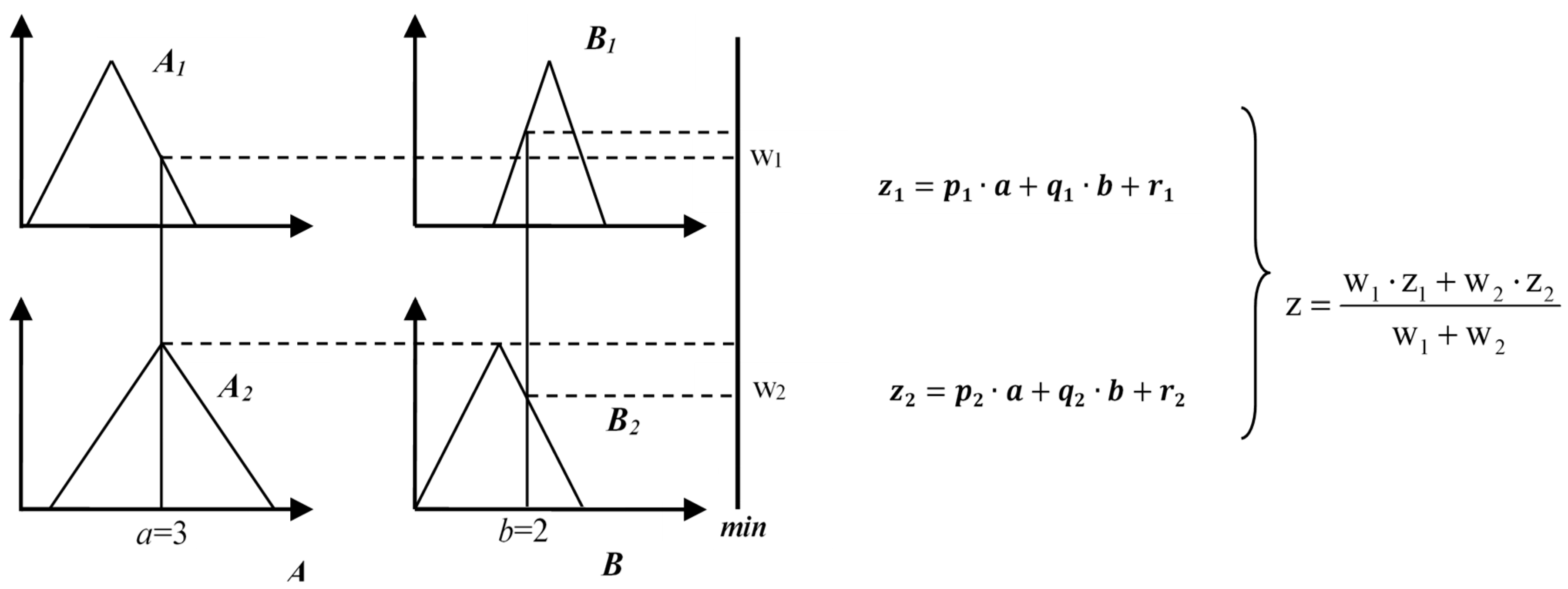
2.2. Adaptive Neuro-Fuzzy Inference System (ANFIS)

The adaptive neuro-fuzzy inference system, developed by Jang, is one of the most popular hybrid neuro-fuzzy systems for function approximation [28]. ANFIS represents a Sugeno-type neuro-fuzzy system. A neuro-fuzzy system is a fuzzy system that uses learning methods derived from neural networks to find its own parameters. It is relevant that the learning process is not knowledge-based but data-driven, as FIR methodology.

The main characteristic of the Sugeno inference system is that the consequent, or output, of the fuzzy rules is not a fuzzy set (as are the inputs of the fuzzy rules) but a function, as shown in Equation (1),

R1: If a is A₁ and b is B₁ then z = p₁ × a + q₁ × b + r₁
R2: If a is A₂ and b is B₂ then z = p₂ × a + q₂ × b + r₂

(1)

where a and b are linguistic variables; A₁, A₂, B₁, and B₂ are linguistic values determined by fuzzy sets on the universe of discourse of A and B, and are represented in the form of membership functions; p₁, q₁, r₁, p₂, q₂, and r₂ are parameters of the output functions.

Figure 5 graphically describes the inference process of a Sugeno model composed by the two rules described in Equation (1). The first step of the Sugeno inference is to combine a given input tuple (in the example of Figure 5: a = 3 and b = 2) with the rule’s antecedents to determine the degree to which each input belongs to each corresponding fuzzy set (left panel of Figure 5). The min operator is then used to obtain the weight of each rule, w_i, which is used in the final output computation, z (right panel of Figure 5). Notice that the Sugeno inference has two differentiated sets of parameters. The first set corresponds to the membership function’s parameters of the input variables. The second set corresponds to the parameters associated with the output function of each rule, that is, p_i, q_i, and r_i.

ANFIS is responsible for automatically adjusting these two sets of parameters by means of two optimization algorithms: back-propagation (gradient descendent) and least square estimation. The back-propagation is used to learn the parameters of the antecedents (membership functions) and the least squares estimation is used to determine the coefficients of the linear combinations in the rules’ consequents. The ANFIS structure is composed of five layers as shown in Figure 6. ANFIS has n input nodes, where n is the number of inputs to the system. In the example of Figure 6, n is 2 and corresponds to a and b.

Layer 1 is the fuzzification layer in which each node represents a membership value to a linguistic term as a Gaussian, triangular, etc. function. The parameters of the selected function are adapted by means of the back-propagation algorithm during the learning stage.

As the values of the parameters change, the membership function of the linguistic terms, A_i and B_i, changes. Layer 2 applies a T-norm operator that performs fuzzy intersection. Layer 3 is a normalization layer that normalizes the strength of all rules, i.e., computes ${\overline{\mathbf{\omega }}}_{\mathit{i}}= \frac{{\mathbf{\omega }}_{\mathit{i}}}{{{\displaystyle \sum }}_{\mathit{i}}{\mathbf{\omega }}_{\mathit{i}}}$. Layer 4 updates the parameters of the consequents of the rules by a learning step based on the least squares approximation algorithm. Finally, Layer 5 performs the summation of the outputs of the nodes in Layer 4. ANFIS is a function of the Fuzzy toolbox that runs under the Matlab environment. For a more detailed explanation of the ANFIS methodology refer to Nauck et al. [28].

3. Fuzzy Approaches for Energy Performance of Buildings Forecasting

3.1. Data Collection

The data used for this study stems from the UCI machine learning repository [18] under the name: Energy efficiency data set. Tsanas and Xifara [17] created the data by generating 768 simulated buildings using Ecotet. Ecotet is a sustainable building design software tool that allows the design of buildings by performing a complete analysis on building energy, thermal performance, and water usage, among other functionalities [29].

All buildings in the simulation have a volume of 771.75 m³, but different surface areas and dimensions. All of them are designed with the newest and most common building materials in the construction industry and with building elements achieving the lowest heat loss through the wall, floor or roof (U-value). The simulation assumes that the buildings are located in Athens, Greece, and are residential buildings.

Three types of glazing areas were used, expressed as percentages of the floor area: 10%, 25%, and 40%. Furthermore, five different distribution scenarios for each glazing area were simulated: (1) uniform: 25% glazing on each side, (2) north: 55% on the north side and 15% on each of the other sides, (3) east: 55% on the east side and 15% on each of the other sides, (4) south: 55% on the south side and 15% on each of the other sides, and (5) west: 55% on the west side and 15% on each of the other sides. In addition, they obtained samples with no glazing areas. Finally, all shapes were rotated to face the four cardinal points.

Each of the 768 simulated buildings can be characterized by eight building parameters, which are summarized in

Table 1. Building parameters used as input variables for the models.

RC	Relative Compactness	OH	Overall Height
SA	Surface Area	O	Orientation
WA	Wall Area	GA	Glazing Area
RA	Roof Area	GAD	Glazing Area Distribution

. These parameters correspond to the input variables.

They also recorded the heating load (HL) and the cooling load (CL), which correspond to the output variables. Basic statistical analysis of the data was also performed, showing that linear modelling techniques are not appropriate for this data, since the scatter and density plots do not follow a Gaussian distribution. As mentioned earlier, the data generated represent with high probability actual real data, enabling energy comparisons between buildings [17]. Moreover, the use of simulated building data is useful and justified when dealing with energy prediction challenges, since it allows us to reduce considerably the time needed to obtain the data, design easily different building configurations and work with a lower level of detail.

3.2. Performance Criteria

In order to test the performance of FIR and ANFIS fuzzy models we use 10-fold cross validation (10-fold CV). Model parameters are obtained using the training subset and model validation is performed using the testing subset. For statistical confidence, the training and testing processes are repeated 100 times to the whole dataset, randomly permuted in each run prior to splitting in training and testing subsets.

Three evaluation criteria are used to evaluate the performance of each of the models. Two of them are error measures, i.e., root mean square error (RMSE) and the mean absolute error (MAE), described in Equations (2) and (3), respectively. These errors have been chosen because they are the ones most frequently used in previous studies [17,19,20,21], and it is intended to compare the fuzzy proposed techniques with the methodologies presented in those works.

$$RMSE=\sqrt{\frac{1}{N}{{\displaystyle \sum }}_{i=1}^N{\left|y_i-{\widehat{y}}_i\right|}^2}$$

(2)

$$MAE=\frac{1}{N}{{\displaystyle \sum }}_{i=1}^N{\left|y_i-{\widehat{y}}_i\right|}^{ }$$

(3)

In Equations (2) and (3), ŷ(t) corresponds to the predicted output, y(t) to the system output, and N is the number of samples. Both RMSE and MAE are commonly used accuracy measures that are useful when comparing different methods on the same data, as is the case in this research. The MAE is a linear score, which means all individual differences are weighted equally in the average. The RMSE gives a relatively high weight to large errors, since the errors are squared before they are averaged. This means that the RMSE is most useful when large errors are particularly undesirable. The MAE and the RMSE can be used together to diagnose the variation in the errors in a set of forecasts.

The third evaluation criteria has the goal to obtain a comprehensive performance measure. To this end, RMSE and MAE measures are combined into a synthesis index, SI, as defined in Equation (4).

$$I= \frac{1}{2}{{\displaystyle \sum }}_{i=1}^2\frac{Mea{s}_i-Mea{s}_{min,i}}{Mea{s}_{max,i}-Mea{s}_{min,i}}$$

(4)

where Meas_i is the performance measure, i.e., RMSE, MAE, and $Mea{s}_{min,i}$ and $Mea{s}_{max,i}$ are the minimum and maximum values of the corresponding measure for the set of prediction models, respectively. The SI range is [0, 1] and values close to 0 indicates a highly accurate prediction model.

3.3. Fuzzy Models Identification

In this section the development of ANFIS and FIR models is described. As mentioned before, in this application we have two output variables: HL and CL. We want to study if it is possible to estimate each output by using the eight input variables that represent different building parameters (see Table 1). Both ANFIS and FIR methodologies allow developing models that have a single output, that is, SISO (single input single output) or MISO (multiple inputs single output) models. Therefore, for each methodology two sets of models are obtained, one for each possible output. We refer to sets of models because for each methodology and each output we obtain a model for each of the 10-fold CV, and this is repeated 100 times. Therefore, 1000 models are obtained and validated for each of the two methodologies and outputs studied.

Both fuzzy approaches need to discretize the quantitative data into qualitative data. To this end, it becomes necessary to define at least two parameters: the number of classes (also called granularity) chosen for each input variable (and also for the output variables in the case of the FIR models), and the shape of the membership functions of the input variables (and also for the output variables in the case of the FIR models).

In this research we decided to discretize the input variables relative compactness (RC), surface area (SA), wall area (WA), and glazing area distribution (GAD) into three classes and roof area (RA), overall height (OH), orientation (O), and glazing area (GA) into two classes. The output variables are discretized into three classes in the case of the FIR models. Remember that ANFIS does not have fuzzy consequents, that is, the rules’ output is a function (see Figure 5). These discretization parameters have been chosen based on the analysis of the data. The variable OH can take only two possible values and is, therefore, represented in two classes. Variables RA, O, and GA can take four different values, and some of these values appear only a few times. A discretization with more than two classes does not enhance the model’s prediction power; instead, a higher number of classes can lead to a curse of dimensionality problem. Therefore, it was found that two classes are enough for these variables to have a good representation and to obtain efficient models. The variables that are discretized into three classes have a uniform distribution in their dimensionality space; therefore, an odd number of classes seem more reasonable. Three is the lowest number of classes that give good results for these variables. A Gaussian shape has been used to discretize all variables, since slightly better results are obtained.

3.3.1. ANFIS Models

In order to obtain ANFIS models it is necessary to define two sets of parameters: one related to the discretization process of the input variables, which has been explained before, and the parameters related to the training process. The parameters needed to perform the training process are: the type of the output function (i.e., constant or linear), the optimization method to train the fuzzy inference system, and the number of training epochs.

ANFIS uses the eight input variables to predict each output, HL and CL, and does not perform any kind of feature selection. In this experiment we use a constant output function, two different numbers of training epochs, and a hybrid optimization method (default option). A constant output has been chosen instead of a linear one because the number of parameters that ANFIS needs to optimize when a linear output function is used causes Matlab to run out of memory. Notice there are 8 input variables, 4 discretized into 3 classes and 4 into 2 classes; therefore, each ANFIS model is composed of a rule set of 3⁴ × 2⁴ = 1296 rules. If the output of each rule is a constant output function then the number of output parameters to be optimized is 1296. However, if each rule has as output a first-order linear function the number of output parameters to optimize becomes higher: 11,664 (= 1296 × 9). Two different values, i.e., 50 and 300, are studied to set the number of epochs. The time needed to run a 10-fold CV using an Intel Core2 Duo (3GHz, 4GB of RAM) during 50 epochs is more than 7 h and during 300 epochs is more than 41 h. However, the errors obtained in both cases are virtually identical, for instance, in the case of the HL the RMSE errors obtained are 0.5205 (50 epochs) versus 0.5203 (300 epochs). Therefore, in this case, it does not make sense to increase more than 50 the number of epochs. With respect to the optimization method, the hybrid approach, i.e., a combination of backpropagation and least square estimation (see Section 2.2), has been chosen because it is the original one designed to optimize ANFIS models, and from our point of view is better suited for this task.

3.3.2. FIR Models

As in the case of ANFIS, the first step in order to obtain the FIR models is to discretize the data by converting quantitative values into fuzzy data. For this reason, it is necessary to specify the two parameters described in the previous section, granularity and shape of the membership functions, as well as a third parameter that refers to the discretization algorithm. Depending on the algorithm chosen, the distribution of the membership functions in the variable space may vary, which has a direct impact to the reasoning process and, therefore, to the model predictions. Contrary to FIR, ANFIS does not have this discretization parameter since ANFIS distributes uniformly all the membership functions that describe a specific variable and then performs an optimization process. Figure 7 shows an example of uniform (upper plot) and non-uniform (lower plot) distribution of the membership functions of a variable.

In this research, based on the observation of the data distribution, the equal with partition (EWP) algorithm has been used for the discretization of the RA and OH variables, and the equal frequency partition (EFP) algorithm is used for the discretization of the rest of the variables. EWP performs a uniform distribution of the membership functions. EFP distributes the membership functions of a variable in such a way that all the classes contain the same number of data points. Visual-FIR allows the modeller to choose between 15 discretization algorithms, some of them belonging to the hierarchical family and others to the fuzzy family [26].

Once the data has been discretized, FIR methodology performs a feature selection process where the most relevant causal relations between the input variables and the output variable are identified. To this end, the model structure identification process of FIR is used, which performs a feature selection based on the entropy reduction measure, as described in Section 2.1.

FIR founds as optimal HL and CL masks the one shown in Figure 8. That means that for both outputs (HL and CL), the features that have higher relevant causal relation with the output are RC (relative compactness) and GA (glazing area). The use of the other variables does not improve the predictive power of FIR models. Therefore, these two variables represent the minimum subset of variables needed to accurately estimate the heating and cooling loads.

4. Results and Discussion

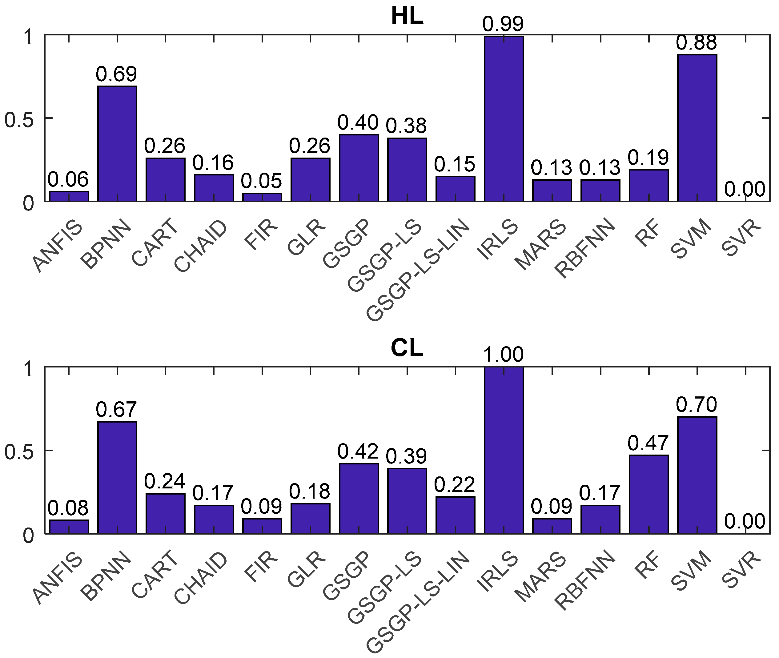
4.1. Fuzzy Approaches Results and Discussion

The RMSE and MAE obtained by ANFIS and FIR models, for both HL and CL output variables, are summarized in the last two rows of

Table 2. RMSE (root mean square prediction errors), MAE (mean absolute prediction errors) and SI (synthesis index) obtained by all the machine learning methodologies, including the fuzzy approaches, ANFIS and FIR, at the bottom of the table. Near the name of each model the reference of the paper is included. The best prediction performances are highlighted.

Model [Reference]	Cooling Load			Heating Load
	MAE	RMSE	SI	MAE	RMSE	SI
IRLS [17]	2.21	3.38	1	2.14	3.14	0.99
RF [17]	1.42	2.57	0.47	0.51	1.01	0.19
SVR [19]	0.89	1.65	0	0.24	0.35	0
GLR [19]	1.29	1.74	0.18	0.79	1.04	0.26
CHAID [19]	1.17	1.86	0.17	0.47	0.91	0.16
CART [20]	1.31	1.94	0.24	0.73	1.11	0.26
SVM [20]	2.10	2.49	0.70	2.19	2.49	0.88
RBFNN [20]	1.30	1.69	0.17	0.51	0.67	0.13
BPNN [20]	1.92	2.63	0.67	1.61	2.25	0.69
MARS [20]	1.12	1.65	0.09	0.53	0.68	0.13
GSGP [21]	1.47	2.36	0.42	1.31	1.06	0.40
GSGP-LS [21]	1.37	2.36	0.39	1.26	1.04	0.38
GSGP-LS-LIN [21]	1.18	2.04	0.22	0.51	0.79	0.15
ANFIS	1.03	1.76	0.08	0.37	0.52	0.06
FIR	1.09	1.72	0.09	0.35	0.49	0.05

. To demonstrate the performance of the developed fuzzy models, we compare the results with those obtained using 13 other techniques, namely IRLS, RF, SVR, GLR, CHAID, CART, SVM, RBFNN, BPNN, MARS, GSGP, GSGP-LS, GSGP-LS-LIN [17,19,20,21]. All these machine-learning methodologies have in common that they generate individual predictive models and are not an ensemble of models. The full results obtained for all the machine-learning approaches are also shown in Table 2.

IRLS is a linear regression algorithm that adjusts weights in the coefficients of the classical regression scheme. RF is a method that builds a set of classification and regression trees using the Bagging algorithm. SVR is a support vector machine that solves regression problems. While other linear regression models try to minimize the error between the predicted and the actual value, SVR tries to fit the best line within a predefined or threshold error value.

GLR, general linear regression, is a more flexible version of standard linear regression that assumes that data points have an arbitrary distribution pattern. CHAID, Chi-squared automatic interaction detector, is a decision tree classification technique that uses the Chi-square as test of independence. The CART is a decision binary tree method of constructing a classification or regression tree according to its dependent variable. The split is chosen using a greedy algorithm to minimize a cost function. The support vector machines, SVM, construct a hyperplane or a set of hyperplanes in a high or infinite dimensional space, which can be used for classification or other tasks like outliers detection. A radial basis function network, RBFNN, is an artificial neural network that uses radial basis functions as activation functions. BPNN is a back-propagation neural network. These networks can be trained with a training dataset propagating the error back to input until the minimal mean square error is achieved. MARS, multivariate adaptive regression splines, fits a basis function (term) to distinct independent variable intervals.

The next three techniques, i.e., GSGP, GSGP-LS and GSGP-LS-LIN, are genetic programming approaches based on evolutionary computation. All of them use geometric semantic operators to produce new candidate solutions. GSGP-LS includes a local search strategy within mutation operator. GSGP-LS-LIN modifies the fitness function including linear scaling. For knowing the parameter settings of these methodologies for the problem at hand refer to [17,19,20,21].

The best prediction performances are highlighted in Table 2. The best results for CL and HL are obtained when the SVR algorithm is used. The second and third best results are obtained by the fuzzy approaches. FIR obtains a slightly better synthesis index (SI) than ANFIS when modelling the HL, whereas for CL it is ANFIS that obtains a slightly better index. Following SVR, FIR and ANFIS performances (with SI lower than 0.1), the next-based alternative is the MARS algorithm. MARS is able to get equivalent performances than FIR for CL, but quite worse for HL. The remaining 12 modelling methodologies have results that are far away from the ones obtained by SVR, FIR and ANFIS.

Figure 9 shows the synthesis indices, SI, obtained for all the modelling methodologies. From this figure it can be seen that IRLS, SVM and BPNN have by far the lowest performance, with SI values higher than 0.65. GSGP and GSGP-LS techniques have poor indices too, i.e., SI values around 0.40. Finally, RF, GLR, CHAID, CART, RBFNN and GSGP-LS-LIN obtain better results than the aforementioned methodologies, with SI values usually lower than 0.24 for CL and 0.26 for HL. However, these results are still away from the values obtained by fuzzy approaches and SVR methodology that are lower than 0.1.

Figure 10 shows real versus predicted ANFIS and FIR results for HL and CL models. In both cases we present the fold that gives larger RMSE, in order to show that even for the worse prediction results, the difference from the real data is almost indistinguishable, especially in the case of the heating load model. Each point in Figure 10 represents a building.

Both models perform well for the task at hand. However, it is important to note the huge difference in computational time between the model identification/training process of ANFIS and FIR methodologies. While ANFIS needs more than 7 h to perform a unique run (for a whole 10-fold CV), FIR needs only a few minutes to perform the same task, both running on the same machine (Intel Core2 Duo, 3 GHz, 4 GB of RAM).

Comparing RMSE versus MAE errors, we can conclude that for both outputs, HL and CL, there is variation in the errors, since $RMSE>MAE$. However, this variation is not sizeable enough to indicate the presence of very significant errors.

Therefore, a first contribution of this research is to show that fuzzy approaches, like ANFIS and FIR, are good alternatives to estimate energy performance of residential buildings based on some building design parameters. Moreover, the fuzzy approaches studied here, have shown better throughput than twelve powerful machine learning approaches well suited for prediction problems.

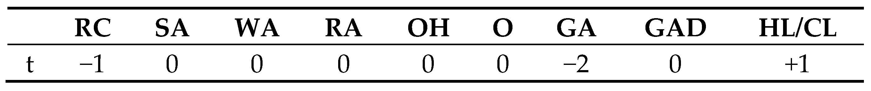
4.2. Feature Selection Results and Discussion

As described in the previous section, FIR finds that two of the eight input variables, RC and GA, have the highest causal relation with the outputs and are enough to predict the heating and cooling loads. This is an interesting result. On the one hand, it is consistent with Tsanas and Xifara’s outcomes that claim the GA is the most important predictor for both HL and CL. On the other hand, it allows the conclusion that the remaining six variables, SA, WA, RA, OH, O and GAD, are redundant or irrelevant. Again, this is consistent with the previous work that concludes variables RC, SA, WA, RA, and OH appear reasonably strongly correlated to the output variables, and also finds that some input variables are highly correlated between them. Based on the FIR feature selection process, it is reasonable to think that the relative compactness variable, RC, includes the information of other relevant variables involved in the study, such as SA or RA. In fact, this makes sense because there is an analytic formula linking RC, SA and the volume [17]. It is clear that the WA variable is directly related to the GA, making it redundant. Therefore, the five variables that appear reasonably strongly correlated to the output variables contain redundant information if RC and GA are already selected.

Based on these results, and with the goal to validate the FIR feature selection process, it has been decided to use the selected features, RC and GA, as the only input variables to find a new ANFIS model. If the rest of the variables are redundant, as the feature selection process of FIR states, ANFIS should be able to model the heating and cooling loads using only RC and GA. Note that the ANFIS models presented in Section 3 used the whole set of input variables. To perform this study, different parameters of the ANFIS methodology are evaluated. Now the number of input variables is reduced from 8 to 2, allowing experimentation with different parameter sets involved in ANFIS modelling: number of epochs (i.e., 50, 100, 500, 1000, 2000) and number of classes of the input variables or partition (i.e., 3-2 and 5-2). All of the experiments use Gaussian membership functions, linear output function, and the hybrid optimization method. Notice that in this experiment it is possible to work with a linear output function since the number of rules for the rule set is 6 in the case that the chosen partition is 3-2, and 10 if the chosen partition is 5-2.

The results obtained for the heating and cooling loads using the different set of parameters and performing an average of the errors obtained when executing the 10-fold CV 100 times are summarized in

Table 3. Prediction errors obtained by ANFIS for the HL, when the features selected by FIR are used as input variables, that is, RC and GA. The best prediction performances are highlighted.

Heating Load	#Epochs	Partition	RMSE	MAE	Exec. Time (min)
	50	3-2	1.71	1.34	0.1
	100	3-2	1.28	0.90	0.2
	500	3-2	1.13	0.85	0.7
	1000	3-2	1.10	0.83	1.3
	2000	3-2	1.09	0.81	2.6
	50	5-2	0.85	0.63	0.2
	100	5-2	0.55	0.40	0.3
	500	5-2	0.51	0.37	1.2
	1000	5-2	0.51	0.37	2.4
	2000	5-2	0.51	0.37	5

and

Table 4. Prediction errors obtained by ANFIS for the CL, when the features selected by FIR are used as input variables, that is, RC and GA. The best prediction performances are highlighted.

Cooling Load	#Epochs	Partition	RMSE	MAE	Exec. Time (min)
	50	3-2	2.57	2.13	0.1
	100	3-2	2.26	1.69	0.2
	500	3-2	2.16	1.68	0.7
	1000	3-2	2.16	1.68	1.3
	2000	3-2	2.15	1.68	2.8
	50	5-2	1.68	1.09	0.2
	100	5-2	1.69	1.09	0.4
	500	5-2	1.69	1.09	1.2
	1000	5-2	1.69	1.09	2.5
	2000	5-2	1.69	1.09	5.1

, respectively.

Comparing Table 2 vs. Table 3 and Table 4 it is clear that there are ANFIS models that reach the same level of accuracy, or even a little higher, than the ANFIS models that use the whole set of 8 features. The best results (shaded cells) are obtained when RC and GA variables are discretized into 5 and 2 classes (5-2), respectively. Fifty epochs is enough to derive a good CL model; increasing the number of optimization steps do not improve the model. The HL models need at least 100 epochs to be optimized properly.

Note that in these experiments a linear output function is always selected. Since the model has only two features, it becomes useful to use those ANFIS parameters that allow a higher tuning level in order to extract as much information as possible from the data available. That is why a 5-2 discretization (instead of the previous 3-2) and a linear output function (instead of the constant previously used) are the parameters that obtain better results. Increasing the granulation to 7-2 does not improve the models obtained. The computational time needed when using only the 2 features selected by FIR is in the order of minutes, not hours, as was the case when all 8 features were used. Specifically, the number of output parameters to be optimized has been reduced from 1296 to only 30. It is relevant to recall that a quick and accurate prediction model is of great importance for buildings design and decision making.

Therefore, a second contribution of this research is to illustrate that FIR methodology is able to identify the key parameters (from a set of building design characteristics) governing the energy use of residential buildings. That is, the model identification process of FIR methodology has been revealed as an efficient feature selection approach which can be used by other modelling methodologies, such as ANFIS, to enhance its skills.

5. Conclusions

The main goal of this work is to study the feasibility of fuzzy approaches to estimate the energy performance of buildings. The characteristics of a building are an important factor in determining the necessities of heating and cooling loads. Therefore, it becomes very useful to determine the most relevant building characteristics, related to the heating and cooling, needed to maintain comfortable indoor conditions in order to design and build energy-efficient buildings. This research starts from a previous study [17], which designed a set of buildings with the aim to predict the heating and cooling load of buildings taking into account variables: relative compactness, surface area, wall area, roof area, overall height, orientation, glazing area and glazing area distribution.

Two fuzzy methodologies have been studied in this research, i.e., the fuzzy inductive reasoning (FIR) and the adaptive neuro-fuzzy inference system (ANFIS). In order to test the generalization performance of FIR and ANFIS fuzzy models we use 10-fold cross validation. The training and testing processes were repeated 100 times to the whole dataset, which was randomly permuted in each run prior to splitting it into training and testing subsets. The results achieved by ANFIS and FIR methodologies were compared to those obtained by thirteen machine learning methodologies presented in previous works, i.e., IRLS, RF, SVR, GLR, CHAID, CART, SVM, RBFNN, BPNN, MARS, GSGP, GSGP-LS, GSGP-LS-LIN [17,19,20,21]. From the results, it can be concluded that SVR, together with the two fuzzy approaches (ANFIS and FIR), works much better than the rest of the methodologies. An interesting result is that the feature selection process of the FIR methodology finds that only two input variables, i.e., relative compactness and glazing area, contain the relevant information needed to accurately predict heating and cooling loads. Obtaining ANFIS and FIR models that use only these two variables, and are just as accurate as the models that use the whole data set of eight input variables, proves this finding. Moreover, these quick and accurate prediction models can be very useful for buildings design and decision making.

References

1. European Commission. Available online: https://ec.europa.eu/energy/en/topics/energy-efficiency/energy-performance-of-buildings (accessed on 14 October 2019).
2. Deloitte. Energy Efficiency in Europe. The Levers to Deliver the Potential. Available online: https://www2.deloitte.com/content/dam/Deloitte/global/Documents/Energy-and-Resources/energy-efficiency-in-europe.pdf (accessed on 15 November 2019).
3. Seyedzadeh, S.; Rahimian, F.; Glesk, I.; Roper, M. Machine learning for estimation of building energy consumption and performance: A review. Vis. Eng. 2018, 6. [Google Scholar] [CrossRef]
4. Alam, A.G.; Baek, C.I.; Han, H. Prediction and Analysis of Building Energy Efficiency Using Artificial Neural Network and Design of Experiments. Appl. Mech. Mater. 2016, 819, 541–545. [Google Scholar]
5. Zhang, Y.; O’Neill, Z.; Dong, B.; Augenbroe, G. Comparisons of inverse modeling approaches for predicting building energy performance. Build. Environ. 2015, 86, 177–190. [Google Scholar] [CrossRef]
6. Ascione, F.; Bianco, N.; De Stasio, C.; Mauro, G.M.; Vanoli, G.P. Artificial neural networks to predict energy performance and retrofit scenarios for any member of a building category: A novel approach. Energy 2017, 118, 999–1017. [Google Scholar] [CrossRef]
7. Benedetti, M.; Cesarotti, V.; Introna, V.; Serranti, J. Energy consumption control automation using Artificial Neural Networks and adaptive algorithms: Proposal of a new methodology and case study. Appl. Energy 2016, 165, 60–71. [Google Scholar] [CrossRef]
8. Ahn, J.; Cho, S.; Chung, D.H. Analysis of energy and control efficiencies of fuzzy logic and artificial neural network technologies in the heating energy supply system responding to the changes of user demands. Appl. Energy 2017, 190, 222–231. [Google Scholar] [CrossRef]
9. Xuemei, L.; Lixing, D.; Jinhu, L.; Gang, X.; Jibin, L. A novel hybrid approach of KPCA and SVM for building cooling load prediction. In Proceedings of the Third International Conference on Knowledge Discovery and Data Mining (WKDD), Phuket, Thailand, 9–10 January 2010; pp. 522–526. [Google Scholar] [CrossRef]
10. Hou, Z.; Lian, Z. An application of support vector machines in cooling load prediction. Intell. Syst. Appl. 2009, 2, 1–4. [Google Scholar] [CrossRef]
11. Jung, H.C.; Kim, J.S.; Heo, H. Prediction of building energy consumption using an improved real coded genetic algorithm based least squares support vector machine approach. Energy Build. 2015, 90, 76–84. [Google Scholar] [CrossRef]
12. Ahmad, M.W.; Mourshed, M.; Rezgui, Y. Trees vs Neurons: Comparison between random forest and ANN for high-resolution prediction of building energy consumption. Energy Build. 2017, 147, 77–89. [Google Scholar] [CrossRef]
13. Tuhus-Dubrow, D.; Krarti, M. Genetic-algorithm based approach to optimize building envelope design for residential buildings. Build. Environ. 2010, 45, 1574–1581. [Google Scholar] [CrossRef]
14. Dounis, A.I.; Caraiscos, C. Advanced control systems engineering for energy and comfort management in a building environment—A review. Renew. Sustain. Energy Rev. 2009, 13, 1246–1261. [Google Scholar] [CrossRef]
15. Lee, W.S. Evaluating and ranking energy performance of office buildings using fuzzy measure and fuzzy integral. Energy Convers. Manag. 2010, 51, 197–203. [Google Scholar] [CrossRef]
16. Nebot, A.; Mugica, F. Fuzzy Approaches Improve Predictions of Energy Performance of Buildings. In Proceedings of the 3rd International Conference on Simulation and Modeling Methodologies, Technologies and Applications, Reykjavík, Iceland, 29–31 July 2013; Volume 1, pp. 504–511. [Google Scholar]
17. Tsanas, A.; Xifara. Accurate quantitative estimation of energy performance of residential buildings using statistical machine learning tools. Energy Build. 2012, 49, 560–567. [Google Scholar] [CrossRef]
18. UCI. Available online: http://archive.ics.uci.edu/ml/ (accessed on 2 October 2019).
19. Chou, J.S.; Bui, D.K. Modeling heating and cooling loads by artificial intelligence for energy-efficient building design. Energy Build. 2014, 82, 437–446. [Google Scholar] [CrossRef]
20. Cheng, M.Y.; Cao, M.T. Accurately predicting building energy performance using evolutionary multivariate adaptive regression splines. Appl. Soft Comput. 2014, 22, 178–188. [Google Scholar] [CrossRef]
21. Castelli, M.; Trujillo, L.; Vanneschi, L.; Popovič, A. Prediction of energy performance of residential buildings: A genetic programming approach. Energy Build. 2015, 102, 67–74. [Google Scholar] [CrossRef]
22. Klir, G.; Elias, D. Architecture of Systems Problem Solving, 2nd ed.; Plenum Press: New York, NY, USA, 2002. [Google Scholar]
23. Nebot, A.; Mugica, F. Fuzzy inductive reasoning: A consolidated approach to data-driven construction of complex dynamical systems. Int. J. Gen. Syst. 2012, 41, 645–665. [Google Scholar] [CrossRef]
24. Nebot, A.; Mugica, F.; Cellier, F.; Vallverdú, M. Modeling and Simulation of the Central Nervous System Control with Generic Fuzzy Models. Simulation 2003, 79, 648–669. [Google Scholar] [CrossRef]
25. Carvajal, R.; Nebot, A. Growth Model for White Shrimp in Semi-intensive Farming using Inductive Reasoning Methodology. Comput. Electron. Agric. 1998, 19, 187–210. [Google Scholar] [CrossRef] [Green Version]
26. Escobet, A.; Nebot, A.; Cellier, F.E. Visual-FIR: A tool for model identification and prediction of dynamical complex systems. Simul. Model. Pract. Theory 2008, 16, 76–92. [Google Scholar] [CrossRef]
27. Shannon, C.E. A Mathematical Theory of Communication. Bell Syst. Tech. J. 1948, 27, 379–423. [Google Scholar] [CrossRef] [Green Version]
28. Nauck, D.; Klawonn, F.; Kruse, R. Neuro-Fuzzy Systems; John Wiley & Sons: Hoboken, NJ, USA, 1997. [Google Scholar]
29. Ecotet. Available online: http://usa.autodesk.com/ecotect-analysis/ (accessed on 23 October 2019).
Figure 1. Fuzzy inductive reasoning (FIR) fuzzification process of human age variable.
Applsci 10 00720 g001
Figure 2. Example of a mask in FIR methodology.
Applsci 10 00720 g002
Figure 3. Derivation of FIR pattern rule base [23].
Applsci 10 00720 g003
Figure 4. FIR prediction process diagram.
Applsci 10 00720 g004
Figure 5. Example of how a Sugeno model works (evaluation of two fuzzy rules with two input variables or antecedents, a = 3 and b = 2) [28].
Applsci 10 00720 g005
Figure 6. Adaptive neuro-fuzzy inference system (ANFIS) architecture [28].
Applsci 10 00720 g006
Figure 7. Example of uniform (upper plot) and non-uniform (lower plot) membership functions distribution.
Applsci 10 00720 g007
Figure 8. FIR mask obtained for heating load (HL) and cooling load (CL) models.
Applsci 10 00720 g008
Figure 9. Synthesis indices (SI) of all machine learning methodologies for the heating load (top figure) and the cooling load (bottom figure). Values lower than 0.1 correspond only to SVR, ANFIS and FIR.
Applsci 10 00720 g009
Figure 10. Real versus ANFIS and FIR prediction results for heating load (upper plot) and cooling load (lower plot) models. Each point in the plot represents a building. The results of the Cooling Load correspond to fold #1 in one of the 10 iterations. MAE and RMSE obtained by the ANFIS model in this fold are 1.08 and 1.76, respectively. MAE and RMSE obtained by the FIR model in this fold are 1.16 and 1.74, respectively. The results of the Heating Load correspond to fold #7 in one of the 10 iterations. MAE and RMSE obtained by the ANFIS model in this fold are 0.54 and 0.68, respectively. MAE and RMSE obtained by the FIR model in this fold are 0.42 and 0.61, respectively.
Applsci 10 00720 g010