1. Introduction
The economic competitiveness of photovoltaic (PV) systems, compared to conventional power production technologies, has continuously improved during the last years. Therefore, they exhibit significant potential for deployment in both stand-alone and grid-connected applications, also in combination with electrical energy storage units [
1].
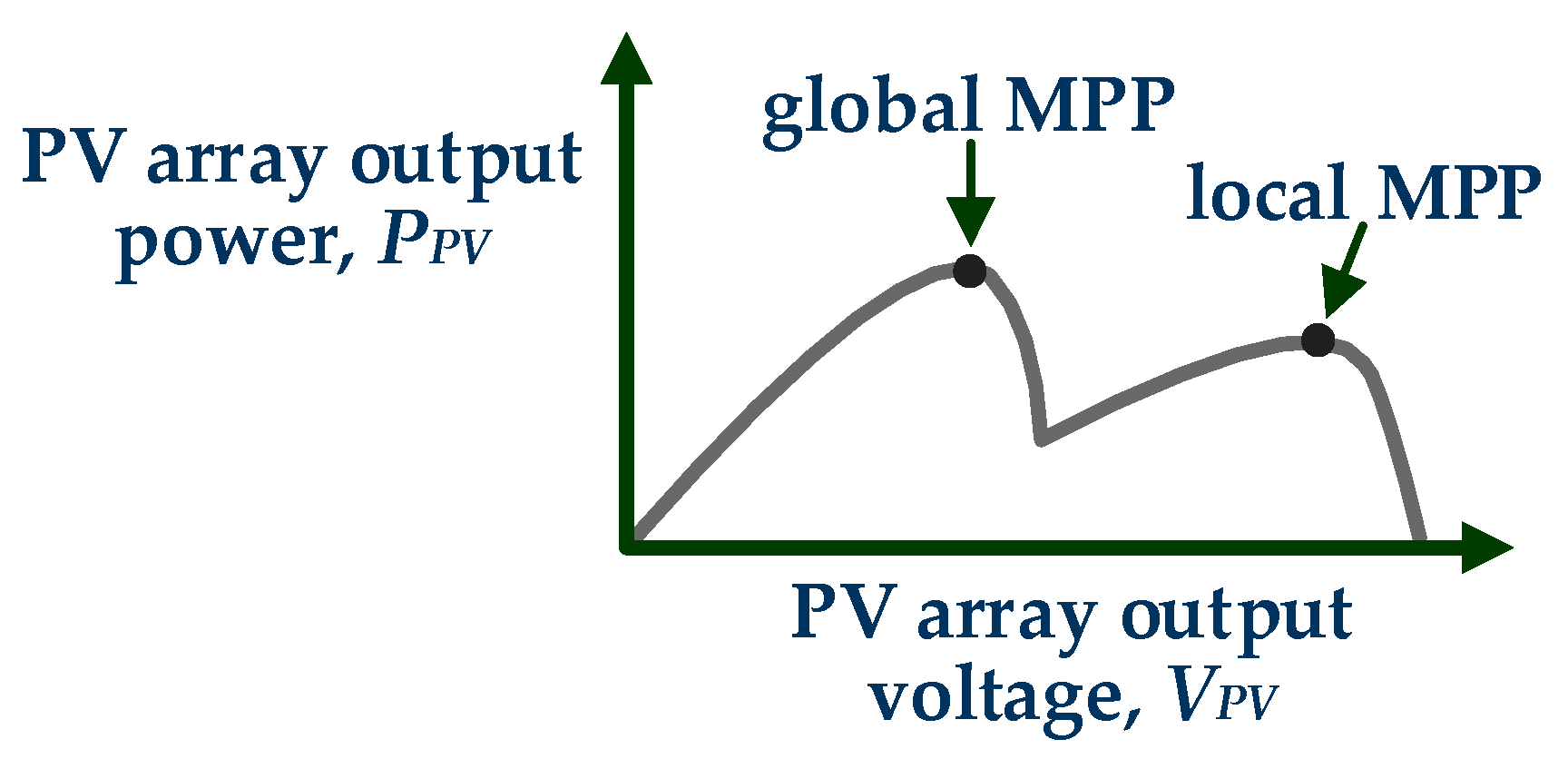
The PV modules comprising the PV array of a PV energy production system may operate under non-uniform incident solar irradiation conditions due to partial shading caused by dust, nearby buildings, trees, etc. As shown in
Figure 1, under these conditions the power–voltage curve of the PV array exhibits multiple local maximum power points (MPPs). However, only one of these MPPs corresponds to the global MPP (GMPP), where the PV array produces the maximum total power [
2]. Therefore, the controller of the power converter that is connected at the output of the PV array must execute an effective global MPP tracking (GMPPT) process in order to continuously operate the PV array at the GMPP during the continuously changing incident solar irradiation conditions. That process results in the continuous maximization of the energy production of the installed PV system and enables the reduction of the corresponding levelized cost of electricity (LCOE) [
1].
The simplest algorithm for detecting the position of GMPP is to scan the entire power-voltage curve of the PV source by iteratively modifying the duty cycle of the PV power converter [
3], which results in the continuous modification of the PV source output voltage. Alternatively, the current–voltage characteristic of the PV array is scanned by iteratively increasing the value of the reference current in a direct current/direct current (DC/DC) PV power converter with average current-mode control [
4]. Compared to the power-voltage scan process, this method has the advantage of faster detection of the GMPP, since it avoids searching the parts of the current-voltage curve located on the left-hand side of the local MPPs. In both of these methods, the accuracy and speed of detecting the GMPP under complex shading patterns depend on the magnitude of the perturbation search-step of the duty cycle or reference current, respectively. In [
5], the current–voltage curve of the PV source is scanned by setting in the ON and OFF states the power switch of a boost-type DC/DC converter, thus causing the PV source current to sweep from zero to the short-circuit value. The PV source current and voltage are sampled at high speed during this process in order to calculate the PV array output voltage where the PV power production is maximized (i.e., GMPP). The effective implementation of this technique requires the use of high-bandwidth current and voltage sensors, a high-speed analog-to-digital converter and a fast digital processing unit [e.g., a field-programmable gate array (FPGA)], thus resulting in high manufacturing cost of the GMPPT controller. Also, the application of this method requires the use of an inductor in series with the PV source, thus it cannot be applied in non-boost type power converter topologies.
The GMPPT algorithms proposed in [
6,
7] are based on searching for the global MPP close to integer multiples of 0.8 × V
oc, where V
oc is the open-circuit voltage of the PV modules. Thus, this technique requires knowledge of both the value of V
oc and the number of series-connected PV modules (or sub-modules with bypass diodes) within a PV string. A GMPPT controller based on machine learning has been proposed in [
8], using Bayesian fusion to avoid convergence to local MPPs under partial shading conditions. For that purpose, a conditional probability table was trained using values of the PV array output voltage at integer multiples of 80% of the PV modules open-circuit voltage under various shading patterns. In [
9], the GMPP search process was based on the value of an intermediate parameter (termed as “beta”), which is calculated according to the PV modules open-circuit voltage and the number of PV modules connected in series in the PV string. All of the techniques described above cannot be applied to PV arrays with unknown operational characteristics. Therefore, they cannot be incorporated in commercial PV power converter products used in PV applications, where the operational characteristics of the PV array are determined by the end-user without having been known during the power converter manufacturing stage.
In [
10] a distributed maximum power point tracking (DMPPT) method is proposed, where the power converters of each PV module communicate with each other in order to detect deviations among the power levels generated by the individual PV modules of the PV array. That process enables the identification of the occurrence of partial shading conditions within the submodules that they comprise. The global MPP is then detected by searching with a conventional maximum power point tracking (MPPT) method (e.g., incremental-conductance) at particular voltage ranges derived similarly to the 0.8 × V
oc GMPPT technique. Therefore, the implementation of this technique requires knowledge of the PV source arrangement/configuration and its operational characteristics.
Evolutionary algorithms have also been applied, considering the GMPPT process as an optimization problem where the global optimum (i.e., GMPP) must be discovered so that the objective function corresponding to the output power of the PV array is maximized. The advantage of these types of algorithm is that they are capable of searching for the position of the GMPP on the power-voltage curve of the PV source with a lower number of search steps compared to the exhaustive scanning/sweeping process. These algorithms have been inspired by natural and biological processes and they differ on the operating principle used to produce the alternative operating points of the PV array, which are investigated during searching for the GMPP position. The particle swarm optimization (PSO) [
11,
12,
13], grey wolf optimization (GWO) [
14,
15,
16], flower pollination algorithm (FPA) [
17,
18], Jaya algorithm [
19] and differential evolution (DE) algorithm [
20] are the most frequently employed evolutionary algorithms. Genetic algorithms (GAs) inspired by the process of natural evolution are applied in [
21]. However, this type of optimization algorithm exhibits high computational complexity compared to other evolutionary algorithms, due to the complex operations (i.e., selection, mutation and crossover) which must be performed during the chromosomes search process.
During operation, the evolutionary algorithms avoid convergence to local MPPs and converge to an operating point that is located close to the GMPP. Thus, they should be combined with a traditional MPPT method [e.g., perturbation and observation (P&O), incremental-conductance (INC) etc.], which is executed after the evolution algorithm execution has been finished, in order to: (i) fine-tune the PV source operating point to the GMPP and (ii) maintain operation at the GMPP during short-term changes of solar irradiation or shading-pattern, which do not alter significantly the shape (e.g., relative position of the local and global MPPs) of the power–voltage curve (e.g., [
15]). This enables to avoid frequent re-executions of the evolutionary algorithm, which would result in power loss due to operation away from the GMPP during the search process. The execution of the evolutionary algorithm is either re-initiated periodically (e.g., every few minutes), or after the detection of significant changes of the PV power production, in order to track any new position of the GMPP. The performance of many metaheuristic optimization techniques implementing the GMPPT process in partially-shaded PV systems has been compared in [
22].
This paper presents a new GMPPT method, which is based on a machine-learning algorithm. Compared to the past-proposed GMPPT techniques, the Q-learning-based method proposed in this paper has the following advantages: (a) it does not require knowledge of the operational characteristics of the PV modules and the PV array comprised in the PV system; and (b) due to its inherent learning capability, it is capable of detecting the GMPP in significantly less search steps. Thus, the proposed GMPPT method is suitable for employment in PV applications, where the shading pattern may change quickly (e.g., wearable PV systems, building-integrated PV systems, where shading is caused by people moving in front of the PV array, etc.). The numerical results presented in this paper, validate the capabilities and advantages of the proposed GMPPT technique.
This paper is organized as follows: the operating principles and structure of the proposed Q-learning-based GMPPT method are analyzed in
Section 2; the numerical results by applying the proposed method, as well as the PSO evolutionary GMPPT algorithm, for various shading patterns of a PV array are presented in
Section 3; and, finally, the conclusions are discussed in
Section 4.
2. The Proposed Q-Learning-Based Method for Photovoltaic (PV) Global Maximum Power Point Tracking (GMPPT)
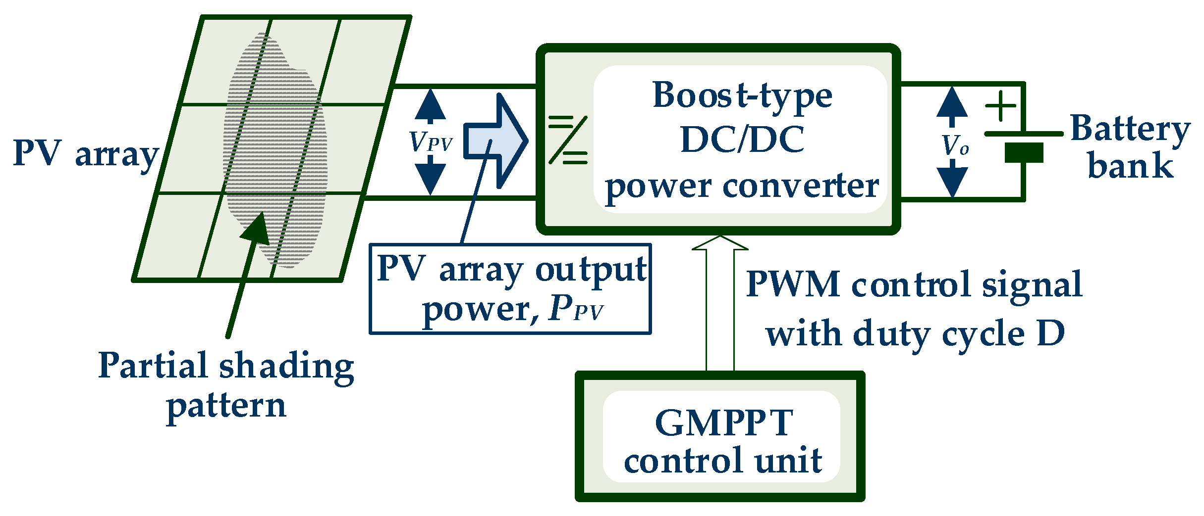
A block diagram of the PV system under consideration is illustrated in
Figure 2. The PV array comprises multiple PV modules connected in series and parallel. The GMPPT process is executed by the GMPPT controller, which produces the duty cycle,
D, of the pulse width modulation (PWM) control signal of the DC/DC converter using measurements of the PV array output voltage and current. Each value of
D determines the PV array output voltage according to (1):
where
(
V) is the DC/DC converter output voltage and
(
V) is the PV array output voltage.
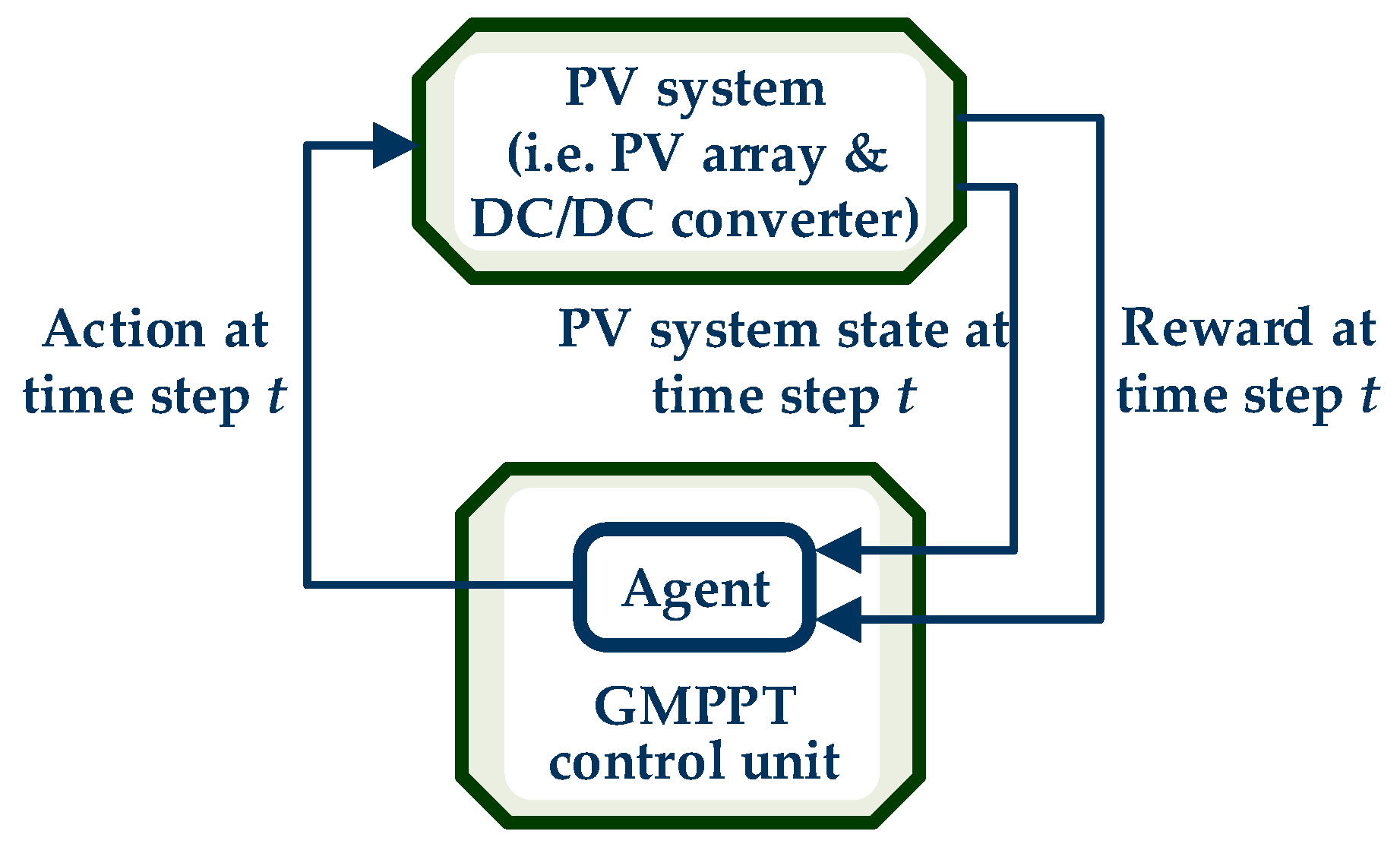
The proposed technique considers the PV GMPPT operation as a Markov decision process (MDP) [
23], which constitutes a discrete-time stochastic control process and models the interaction between an agent implemented in the GMPPT control unit and the PV system (i.e., PV array and DC/DC power converter). The MDP consists of: (a) the state-space
S, (b) the set of all possible actions
A, and (c) the reinforcement reward function, which represents the reward, when applying action
a in state
, which leads to a transition to state
[
23]. The Markovian property dictates that each state transition is independent of the history of previous states and actions and depends only on the current state and action; likewise, each reward is independent of the past states, actions, and rewards and depends only on the most recent transition. A temporal-difference Q-learning algorithm is applied for solving the PV GMPPT optimization problem. The Q-learning algorithm’s goal is to derive an action selection policy, which will maximize the total expected discounted rewards that the system will receive in the future. A simplified representation of process implemented by the Q-learning algorithm in order to control a PV system for the implementation of the GMPPT process is presented in
Figure 3.
In Q-learning, an agent interacts with the unknown environment (i.e., the PV system) and gains experience through a specific set of states, actions and rewards encountered during this interaction [
24,
25,
26,
27]. Q-learning strives to learn the Q-values of state-actions pairs, which represent the expected total discounted reward in the long term. Typically, experience for learning is recorded in terms of samples (
St,
at,
Rt,
St+1), meaning that at some time step
t, action
at was executed in state
St and a transition to the next state
St+1 was observed, while reward
Rt was received. The Q-learning update rule, given a sample (
St,
at,
Rt,
St+1) at time step
, is defined as follows:
where
is the Q-value of the current state-action pair that will be updated,
is the Q-value of the next state-action pair,
is the learning rate,
is the immediate reward and
is the discount factor.
In each time-step, the agent observes its current state and chooses its action according to its action-selection policy . After the action selection, it observes its future state . Then, it receives an immediate reward and selects the future Q-value that offers the maximum value over all possible actions, i.e., . The learning rate determines how much the new knowledge acquired by the agent will affect the existing estimate in the update of .
2.1. Action Selection Policy
Each possible pair of state-action must be evaluated for each state that the agent has visited in order to ensure that the estimated/learned Q-value function is the optimal one (i.e., corresponds to the most suitable action policy). In this work, the Boltzmann exploration policy has been used [
28]. Each possible action has a probability of selection by the agent, which is calculated as follows:
where
is the Boltzmann exploration “temperature”,
is the
i-th possible action,
(size of the action-space) is the total number of alternative actions in each state and
is the Q-value for the
i-th action in state
.
The temperature function is given by:
where
,
are the minimum and maximum, respectively, “temperature” values,
is the current number of visits of the agent in the specific state and
is the maximum number of visits of the agent.
The value of
is positive and controls the randomness of the action selection. If the value of
is high, then all values of the probabilities of each action, which are calculated using (3), are similar. This results in a random action selection depending on the parameter
, which is a random number in the range (0, 1).
Section 2.6 presents the way that
affects the action-selection policy. As the number of visits,
, to a specific state increases, the value of
reduces. After a certain number of visits,
, the value of
becomes equal to its minimum value. This means that the exploration process has been accomplished in that state and the agent chooses the action with the highest Q-value in that state.
2.2. State-Space
During the execution of the PV GMPPT process, each state depends on the current value of the duty cycle of the DC/DC power converter (
Figure 2), the power generated by the PV array and the duty cycle during the previous time-step [
28]:
where
is the number of equally quantized steps of the duty cycle (
) range,
is the number of equally quantized steps of the PV array output power (
) range and
is the number of equally quantized steps of the duty cycle range for the previous time-step
. Selecting high values for
,
and
will result in a higher accuracy of detecting the MPP, but the learning time and storage requirements are increased. For each value of
, the state is determined jointly by the current and the previous quantization steps that the duty cycle value belongs to, as well as by the quantization step that the PV array output power value belongs to. For example, assume that
,
,
,
, the duty cycle value at the current time-step is equal to 0.64, the PV array output power is equal to 53 W and the duty cycle value at the previous time-step equals 0.5. In this case, the agent’s state is equal to (7, 6, 3), because 53 W belongs to the 6th quantization step of the PV power range, 0.64 belongs to the 7th quantization step of the current duty cycle range and 0.5 belongs to the 3rd quantization step of the previous-duty-cycle range.
2.3. Action-Space
The action-space of the PV system GMPPT controller is expressed by the following equation:
where
is the duty cycle for the next time-step,
is the current duty cycle value and
indicates the “increment”, “decrement” or “no-change” of the current duty cycle value.
If the agent selects action “no change”, then it will remain in the same state during the next time-step. The actions “increment” and “decrement” of the current duty cycle value are further classified as “low”, “medium” and “high”, as analyzed in
Section 3, in order to ensure that most of the duty cycle values are selected. Thus, there is a total of seven actions in the action-space with the “no change” action being the last one. This is necessary in order to minimize the probability that the agent will converge to a local MPP. Each action is selected according to the Boltzmann exploration policy, which was analyzed in
Section 2.1. When the exploration process has been finished, the action with the highest Q-value is selected for that particular state. It is considered that the GMPP of the PV array is detected when the action “no change” has the highest Q-value. In this case, the Q-values of all other actions are lower due to the reduction of the PV array output power by the selection of the corresponding actions compared to the Q-value for action “no change”.
2.4. Reward
The criterion for the selection of the most suitable action is the immediate reward,
, which evaluates the action selection according to:
where
is the PV array output power at time step
and
is the desired power difference considered necessary in order for the agent to realize that a significant power change has occurred. In case the difference
is higher than
, then a small positive reward will be given for that specific pair of state-action, in order to “encourage” the agent to continue this map-selection strategy during the next time-step that it will visit the current state. If
is within
it is considered that there is no change in the generated power, and the reward will be equal to zero. Lastly, if
is lower than
, then a small negative reward will be given to the agent such that in the next time-step that the agent will visit the current state again, the action that caused the power reduction will have a small probability of re-selection according to (3). This will result in the selection of actions which promote the increment of the PV array power production during the GMPP exploration process.
2.5. Discount Factor and Learning Rate
The discount factor is a value which is used to balance immediate and future rewards. The agent is trying to maximize the total future rewards, instead of the immediate reward. It is used to adjust the weight of the reward of the current optimal value and indicate the significance of future rewards [
24]. The discount factor is necessary in order to help the agent find optimal sequences of future actions that lead to high rewards soon and not only the current optimal action.
A visit frequency criterion is applied for ensuring that the proposed Q-learning-based GMPPT process will converge to the GMPP. The agent is encouraged to consider that knowledge acquired from states with a small number of visits is more important than knowledge acquired from states with a higher number of visits. Thus, states that have been visited fewer times will have a higher learning rate than states that have been explored more times. This is accomplished by calculating the value of the learning rate
in (2) as follows:
where
,
and
are factors which determine the initial learning rate value for a state with no visits and
is the number of times that the agent visited the specific state. The rationale behind the variable value of alpha is that its value decreases as the number of visits increases to enable convergence in the limit of many visits.
2.6. The Overall Q-Learning-Based GMPPT Algorithm
A flowchart of the overall Q-learning-based PV GMPPT algorithm, which is proposed in this paper, is presented in
Figure 4. The PV GMPPT process is performed as follows:
Step 1: Q-table initialization. As analyzed in
Section 2.2, a Q-table is created using four dimensions according to (5); three dimensions for the state and one for the action. This table is initially filled with zeros, because there is no prior knowledge. Also, a table that contains the number of visits of each state is defined. The size of this table is equal to the number of states. Lastly, an initial value is given to the duty cycle.
Step 2: After the PV array output voltage and current signals reach the steady-state, the PV array-generated power is calculated. According to the value of the duty cycle in the current time-step, its value during the previous time-step and the PV array-generated power, the state is determined using (5).
Step 3: The learning rate is calculated by (8).
Step 4: The temperature τ is calculated by (4) and the probability of every possible action for the current state is also calculated by (3).
Step 5: If the number of visits to the current state is higher than or equal to the predefined value of and the Q-value for the action corresponding to “no-change” of the duty cycle value is the maximum compared to the other actions, then it is concluded that convergence to an operating point close to the GMPP has been achieved and operation at the local MPPs has been avoided. Then, the proposed GMPPT process executes the P&O MPPT algorithm in order to help the agent fine-tune its operation at the GMPP.
Step 6: If the number of visits of the current state is lower than
or if the Q-value for the action corresponding to “no-change” of the duty cycle value is not the maximum, a number in the range (0, 1) is randomly selected and compared to the probabilities of every possible action for the specific state (step 4). Each probability encodes a specific duty cycle change, as follows:
where
(
k = 1, 2, …6) is the probability of each possible action for the current state that is calculated by using (3), while
is a random number in the range
.
Step 7: After the change of the action, a new duty cycle value is applied to the control signal of the DC/DC power converter and the algorithm waits until the PV array output voltage and the current signals reach the steady state. Then, the proposed GMPPT algorithm calculates the difference between the power produced by the PV array at the previous and the current time-steps, respectively, and assigns the reward according to (7).
Step 8: The future state is determined and the Q-function is updated according to (2).
Step 9: Return to step 2.
3. Numerical Results
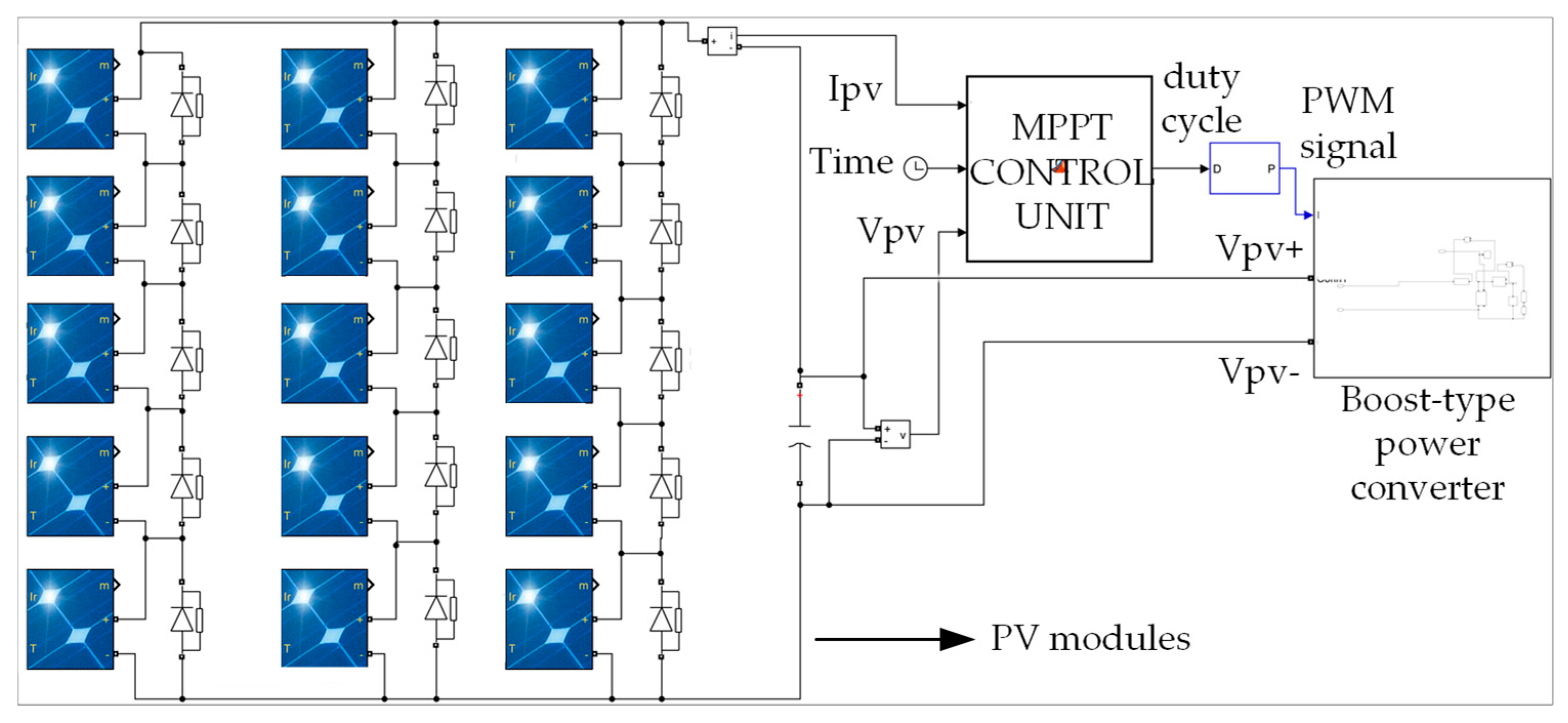
In order to evaluate the performance of the proposed Q-learning-based PV GMPPT method, a model of the PV system has been developed in the MATLAB
TM/Simulink software platform (
Figure 5). The PV system under study consists of the following components: (a) a PV array connected according to the series-parallel topology, (b) a DC/DC boost-type power converter [
29], (c) a GMPPT control unit which produces the duty cycle of the power converter PWM control signal, and (d) a battery that is connected to the power converter output terminals.
Table 1 presents the operational characteristics οf the PV modules comprising the PV array.
Table 2 displays the values of the operational parameters of the proposed Q-learning-based GMPPT method, while
Table 3 presents the action-space that was used for the Q-learning-based method. For each state, the action of Δ
D “increment” or “decrement” with the highest Q-value is performed, in order to ensure the detection of the GMPP with the minimum number of time-steps. There are three categories of duty cycle change (i.e., “low”, “medium” and “high”), which may be selected depending on how close the agent is to the GMPP. The action of “no change” of Δ
D is used such that the agent is able to realize that the position of GMPP has now been detected. The operation of the PV system with the proposed Q-learning-based GMPPT method was simulated for 9 different shading patterns of the PV array. Regarding the state-space, the duty cycle was quantized in 18 equal steps, the PV array output power was quantized in 30 equal steps and the duty cycle value of the previous time-step was quantized in 9 equal steps. For comparison with the proposed method, the PSO-based GMPPT method [
30] was also implemented and simulated as analyzed next.
Table 4 displays the values of the operational parameters of the PSO-based GMPPT method. The values of the operational parameters of the proposed and PSO-based GMPPT algorithms (i.e.,
Table 2,
Table 3 and
Table 4) were selected, such that they converge as close as possible to the global MPP and with the minimum number of search steps for the partial shading patterns under consideration, which are presented in the following section.
3.1. Shading Patterns Analysis
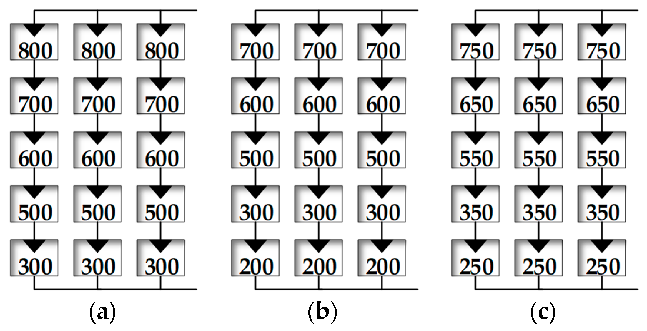
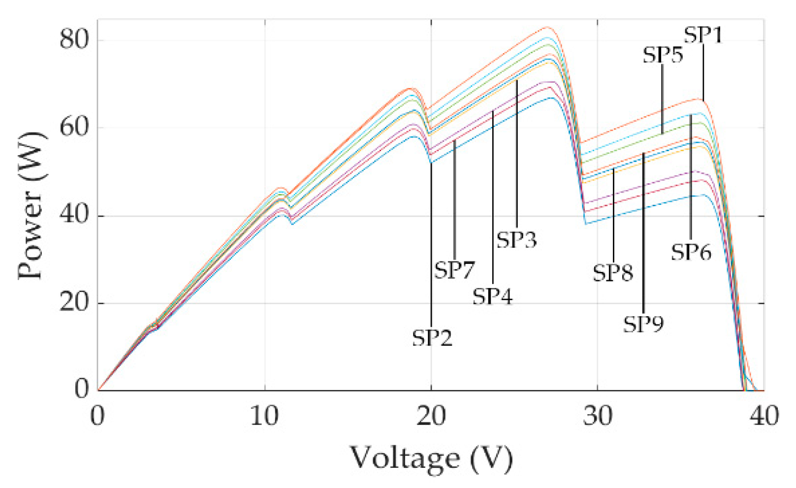
In order to evaluate the performance of the proposed Q-learning-based GMPPT method, the shading patterns 1–3 were used during the learning process and then the acquired knowledge was exploited during the execution of the GMPPT process for the rest of the shading patterns. The distribution of incident solar irradiation (in
) over each PV module of the PV array for each shading pattern is presented in
Figure 6, while the resulting output power-voltage curves of the PV array are presented in
Figure 7. Each number (i.e., SP1, SP2 etc.) in
Figure 7 indicates the order of application of each shading pattern during the test process. These shading patterns, as well as their sequence of application, were formed such that the power-voltage characteristic of the PV array exhibits multiple local MPPs at varying power levels (depending on the shading pattern). This approach enabled the learning capability of the agent employed in the proposed Q-learning-based GMPPT technique and its effectiveness in reducing the time required for convergence to the GMPP to be investigated.
3.2. Tracking Performance of the Proposed Q-Learning-Based GMPPT Method
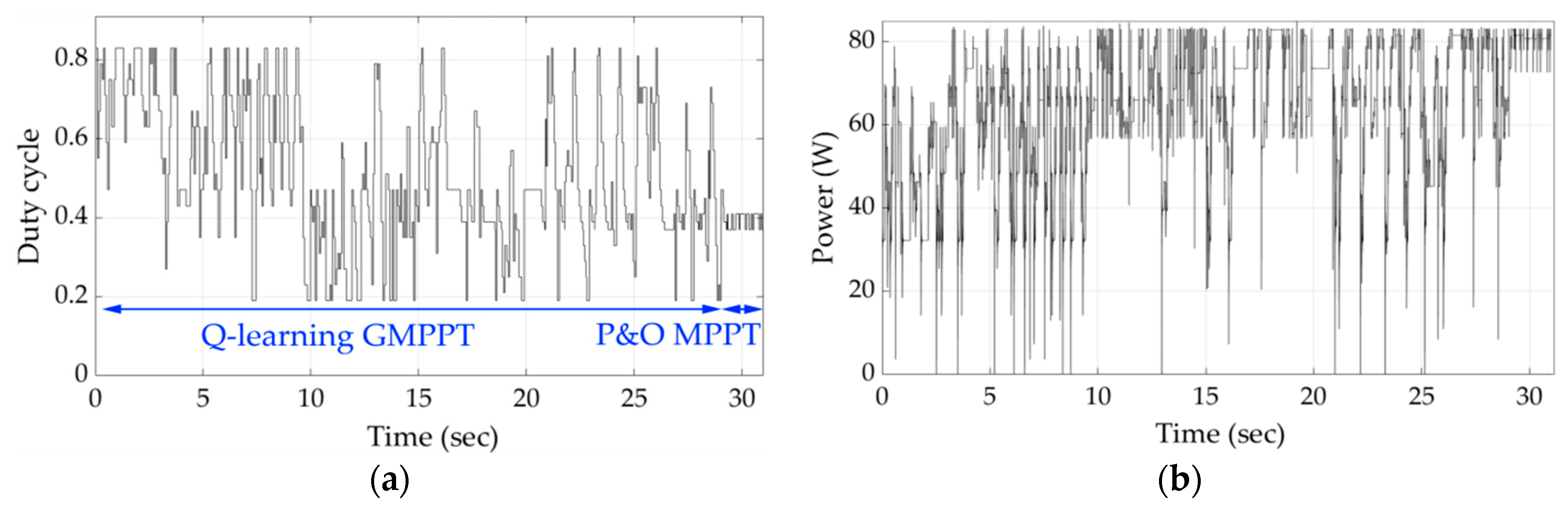
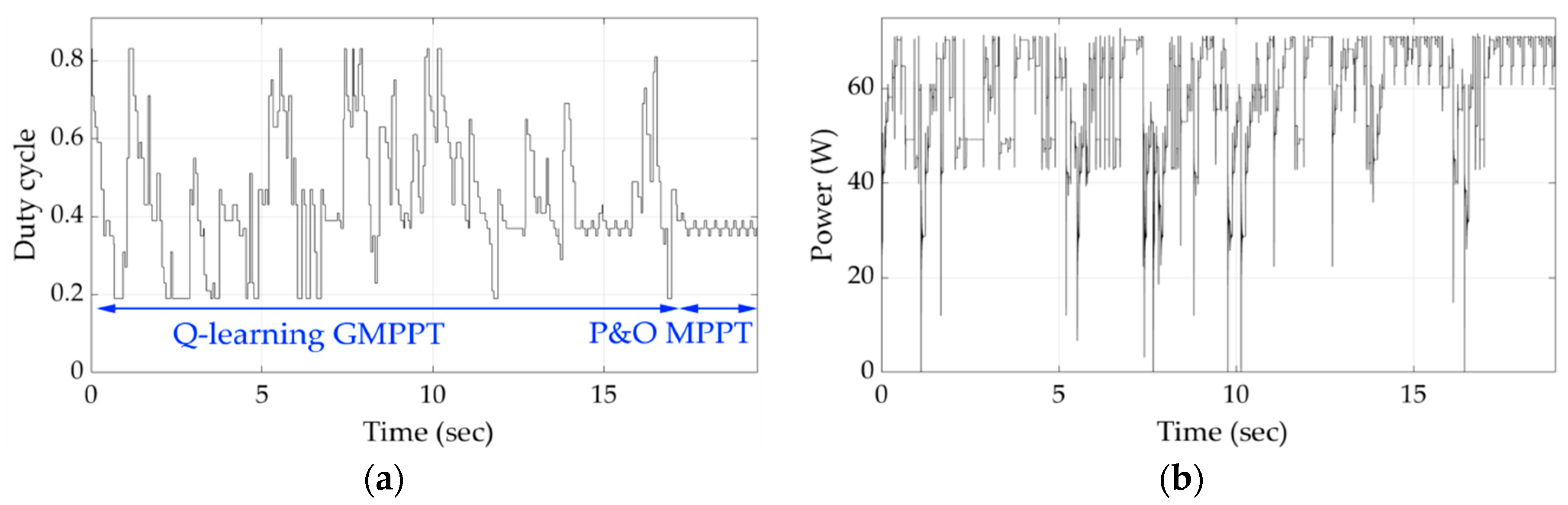
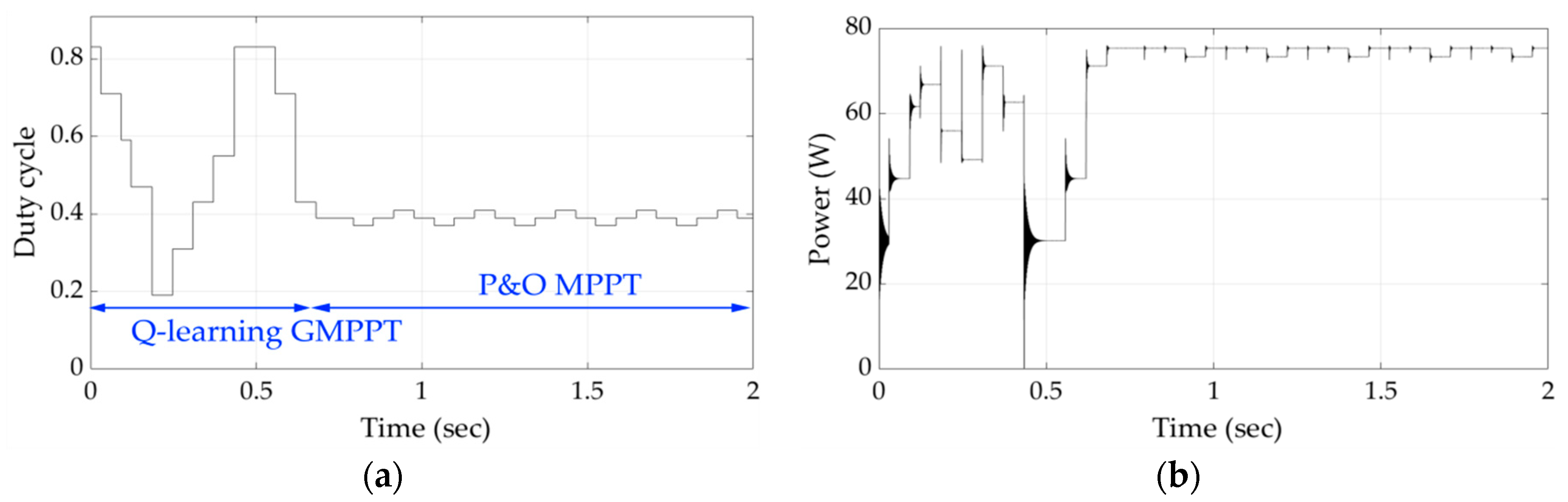
Figure 8 presents the variations of the duty cycle and PV array output power during the execution of the proposed Q-learning-based GMPPT process for shading pattern 1. It is observed that, in this case, the Q-learning-based GMPPT algorithm needed a relatively long period of time in order to converge close to the GMPP. This is due to the fact that initially the agent has no prior knowledge of where the GMPP may be located at. Thus, it has to visit many states, until it converges to the duty cycle value, which corresponds to an operating point close to the GMPP. When the oscillations start (i.e., time = 29 s), the exploration by the agent of the Q-learning-based GMPPT algorithm stops and the P&O MPPT algorithm starts its execution.
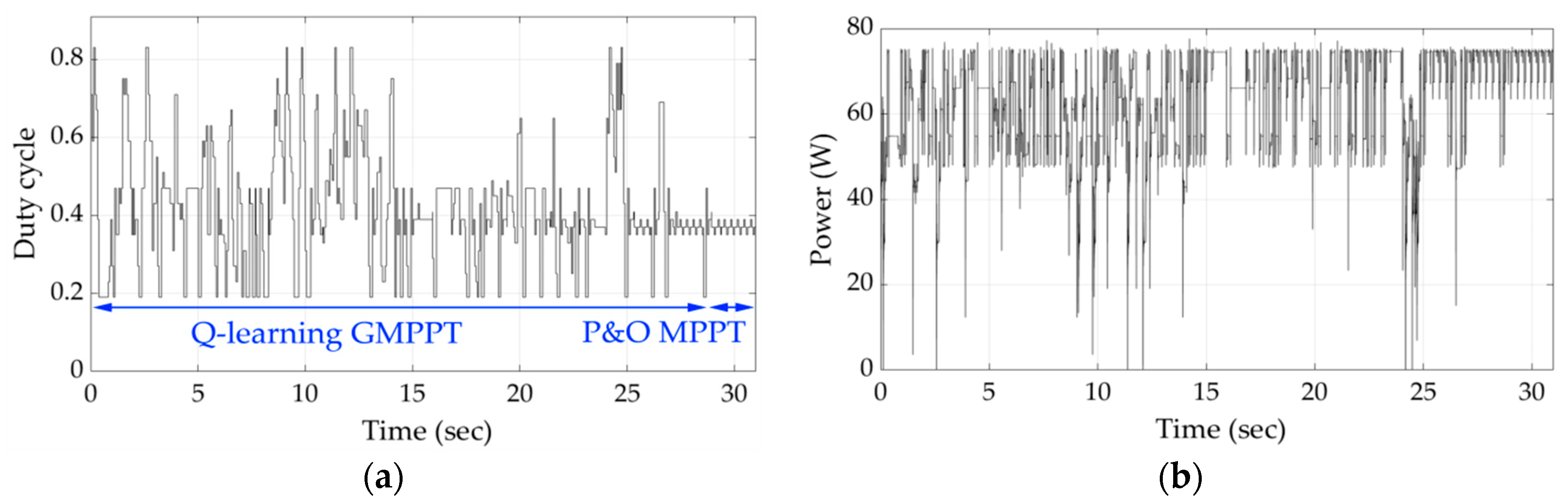
Figure 9 and
Figure 10, respectively, illustrate the duty cycle and PV array output power versus time during the execution of the proposed Q-learning-based GMPPT process for shading patterns 2 and 3. The knowledge gained by the agent during the execution of the GMPPT process for shading pattern 1 did not affect the speed of the GMPP location-detection process for shading pattern 2, since the agent needs to be trained in more shading patterns. Similarly, the knowledge gained during the GMPPT process for shading patterns 1 and 2 did not affect the GMPPT process for locating the GMPP for shading pattern 3. The variations of duty cycle and PV array output power versus time for shading pattern 4, which corresponds to an intermediate power-voltage curve with respect to those of shading patterns 1–3 (
Figure 7), are displayed in
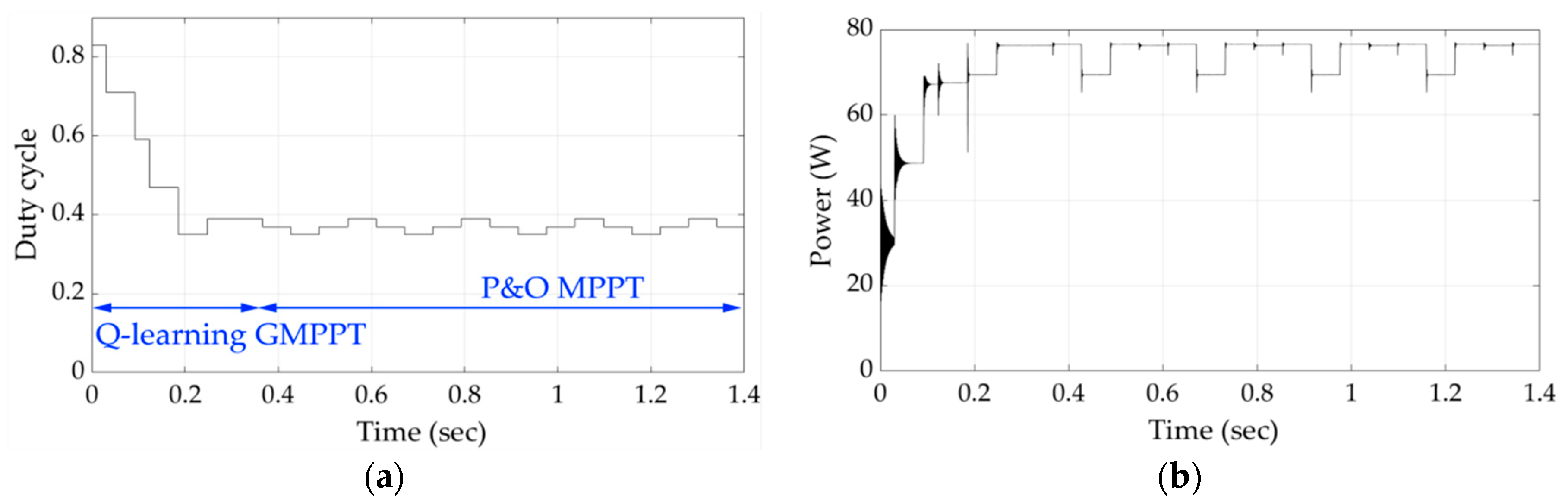
Figure 11. Since the GMPPT process for shading patterns 1–3 had been executed previously, the agent was now able to detect the GMPP in a shorter period of time by exploiting the knowledge acquired before. As shown in
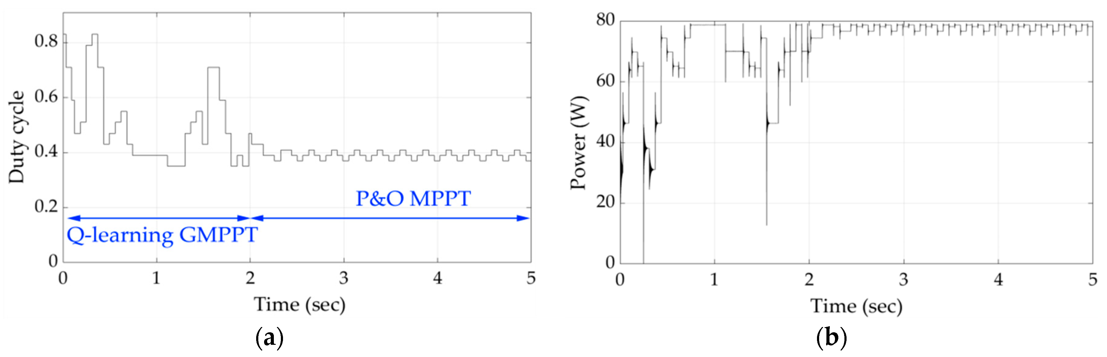
Figure 12, when shading pattern 5 was applied, which was unknown till that time, the time required for detecting the position of the GMPP was further reduced.
Figure 13 and
Figure 14 present the results of the simulations for shading patterns 6 and 7. After this point, the agent of the Q-learning-based GMPPT process is able to detect the GMPP in unknown intermediate power–voltage curve conditions with respect to those of shading patterns 1 and 2 (
Figure 8 and
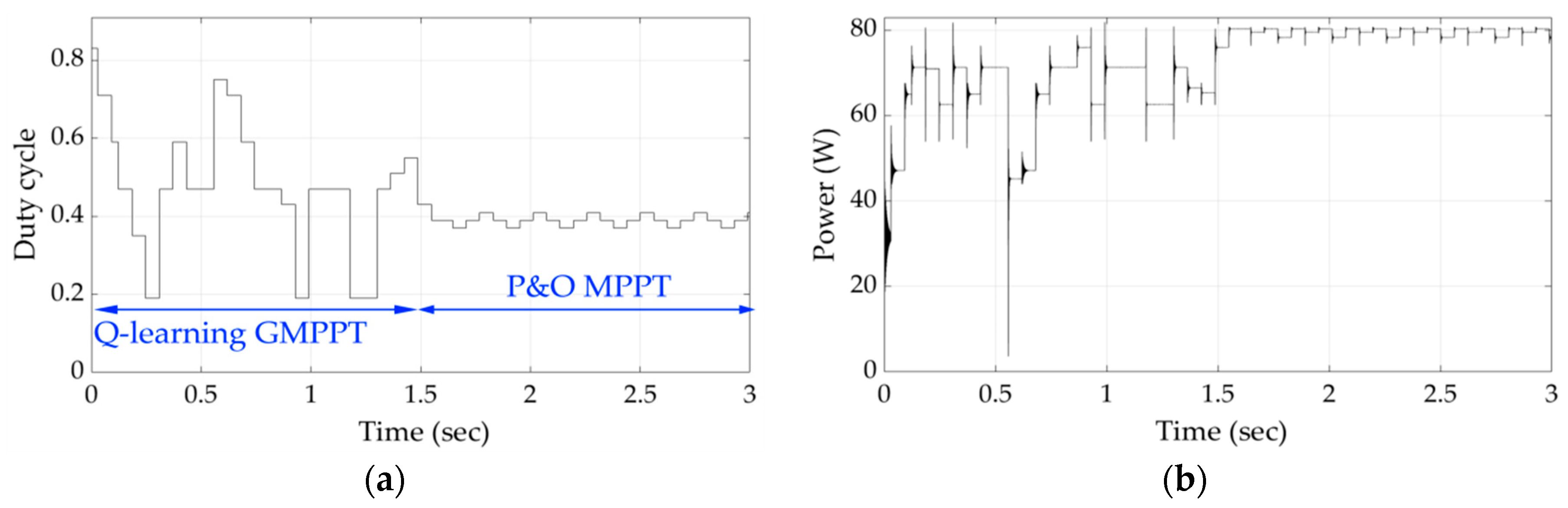
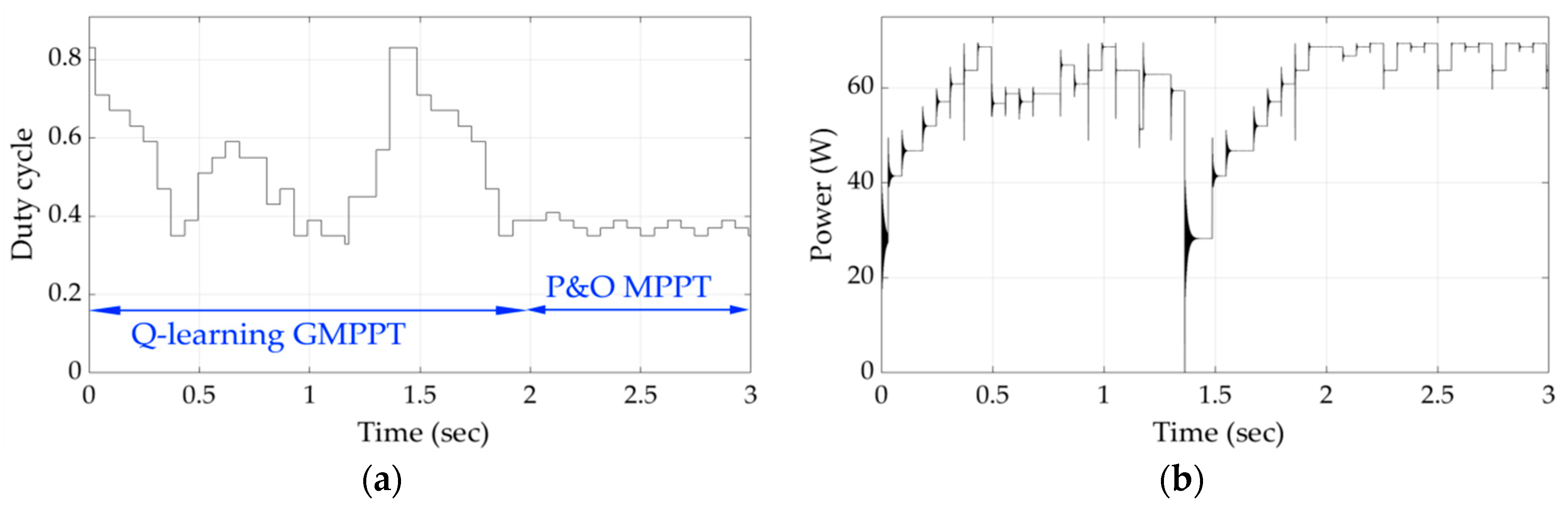
Figure 9) in much less time compared to the previous shading patterns. This happens because the agent had previously acquired enough knowledge from the learning process performed during the GMPPT execution for shading patterns 1–5.
Finally, the simulation results for the unknown shading patterns 8 and 9 in
Figure 15 and
Figure 16, respectively, demonstrate that the agent is capable to detect the GMPP in significantly less time. It is therefore concluded that the inherent learning process integrated in the proposed Q-learning algorithm enhances significantly the convergence speed of the proposed GMPPT method.
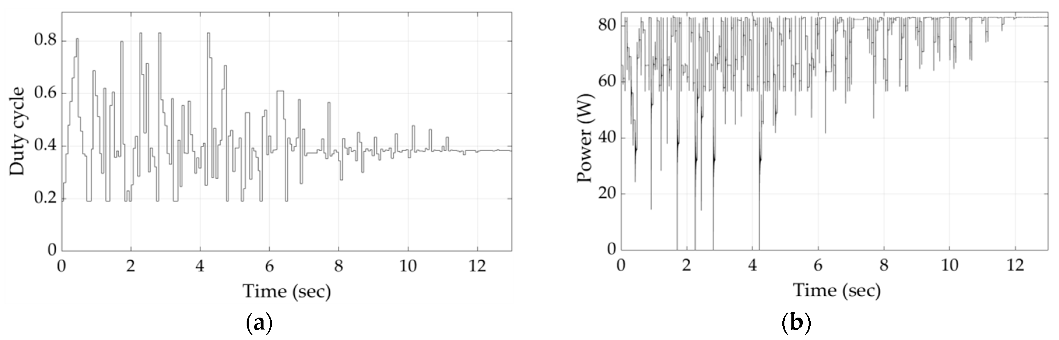
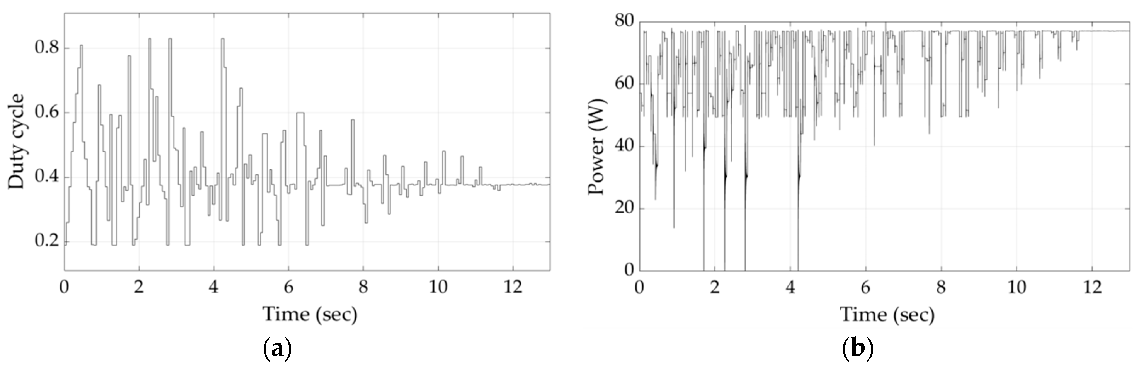
3.3. Tracking Performance of the Particle Swarm Optimization (PSO)-Based GMPPT Method
The PSO GMPPT process was also applied for shading patterns 1–9. As an indicative example,
Figure 17 and
Figure 18 illustrate the duty cycle and PV array output power variations during the execution of the PSO-based GMPPT algorithm for shading patterns 1 and 9, respectively. It can be observed that the variability of the duty cycle and the PV array output power are not affected significantly by the shape of the shading pattern applied. In contrast, as illustrated in
Figure 8,
Figure 9,
Figure 10,
Figure 11,
Figure 12,
Figure 13,
Figure 14,
Figure 15 and
Figure 16, the learning capability of the agent incorporated in the proposed Q-learning-based GMPPT approach enabled the progressive reduction of the duty cycle and the PV array output power variability, when shading patterns 1–9 were applied. The PSO-based GMPPT method required a constant period of time (approximately 11.5 s) in order to detect the location of the GMPP. A similar behavior of the PSO-based algorithm was also observed for shading patterns 2–8.
3.4. Comparison of the Q-Learning-Based and PSO-Based GMPPT Methods
The time required for convergence, the number of search steps performed during the GMPPT process until the P&O process starts its execution and the MPPT efficiency were calculated for each shading pattern for both the Q-learning-based and PSO-based GMPPT algorithms. The execution of the P&O MPPT process was not included in this analysis. The corresponding results are presented in
Table 5 and
Table 6, respectively. The MPPT efficiency is defined as follows:
where
is the PV array output power after convergence of the Q-learning-based, or the PSO-based GMPPT method, respectively and
is the GMPP power of the PV array for the solar irradiance conditions (i.e., shading pattern) under study.
The results presented in
Table 5 indicate that the knowledge acquired initially by the Q-learning agent during the learning process performed when executing the proposed GMPPT algorithm for shading pattern 1 does not affect the number of search steps required when applying shading patterns 2 and 3, respectively. After the learning process of shading patterns 1–3 has been accomplished, the agent needs less time in order to detect the GMPP location for shading pattern 4, which was unknown till that time, with an MPPT efficiency of 99.7%. At that stage, the agent knows how to react when the unknown shading patterns 5–7 are applied, which further reduces significantly the number of search steps required to converge close to the GMPP. Finally, after the execution of the proposed GMPPT algorithm for shading patterns 1–7, the agent needed only 12 and 4 search steps, respectively, when shading patterns 8 and 9 were applied, which were also unknown till that time, and simultaneously achieved an MPPT efficiency of 99.3%–99.6%. Therefore, it is clear that the training of the agent was successful and the subsequent application of the P&O MPPT process is necessary only for compensation of the short-term changes of the GMPP position without re-execution of the entire Q-learning-based GMPPT process.
As demonstrated in
Table 6, the PSO-based GMPPT algorithm needs 11.3–11.6 sec in order to detect the position of the GMPP for each shading pattern, with an MPPT efficiency of 99.6%–99.9%. This is due to the fact that each time that the shading pattern changes, the positions of the particles comprising the swarm are re-initialized and any prior knowledge that was acquired about the location of the GMPP is lost. In contrast, due to its learning capability, the proposed Q-learning-based GMPPT algorithm reduced the convergence time when shading patterns 5–9 were applied by 80.5%–98.3%, compared to the convergence time required by the PSO-based GMPPT process to detect the GMPP with a similar MPPT efficiency.
The MPPT efficiency achieved by the proposed Q-learning-based GMPPT algorithm was lower than that of the PSO-based algorithm by 1.3% when shading pattern 1 was applied, since the learning process was still in evolution. However, the application of a few additional shading patterns (i.e., shading patterns 2–7) offered additional knowledge to the Q-learning agent. Therefore, the resulting MPPT efficiency had already been improved during application of shading patterns 8 and 9 and reached a value similar to that obtained by the PSO-based algorithm, but with significantly less search steps, as analyzed above.
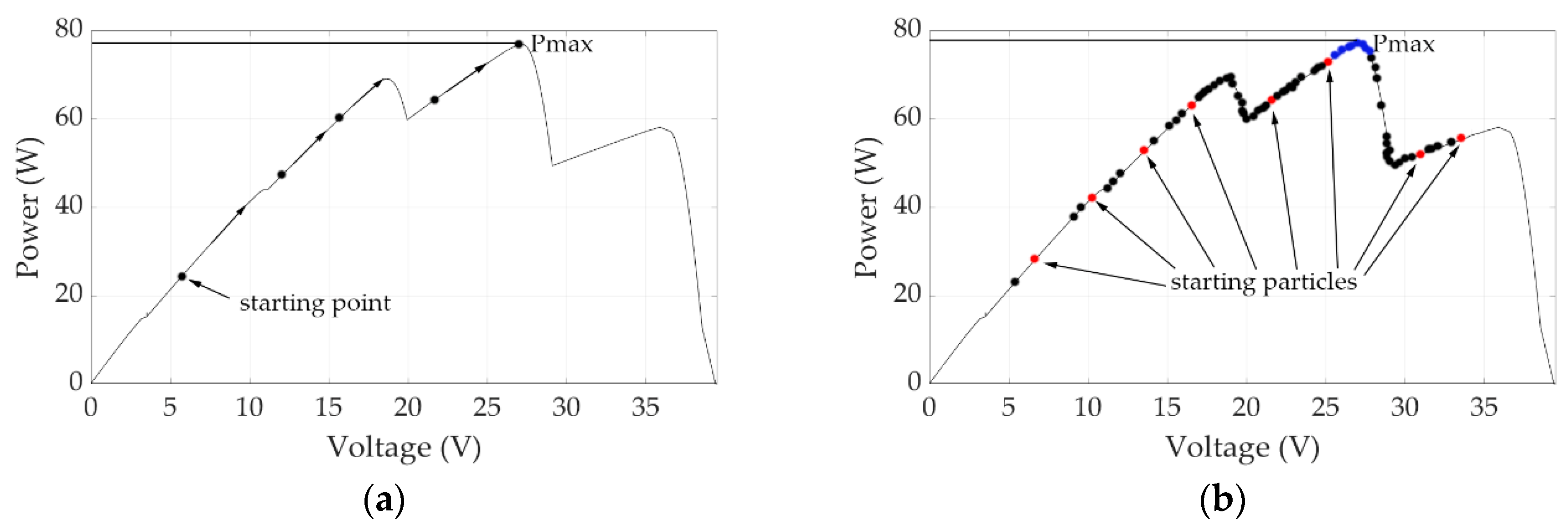
Figure 19a presents an example of the trajectory followed during the PV array output power maximization process, when the proposed Q-learning-based GMPPT method is applied for shading pattern 9.
Figure 19b illustrates the initial positions of the particles comprising the PSO swarm (red dots), the positions of the particles during all intermediate swarm generations (black dots), as well as their final positions (blue dots) for the same shading pattern. It is observed that the PSO algorithm must visit a large number of alternative operating points of the PV array in order to be able to detect the position of the GMPP with an MPPT efficiency similar to that of the proposed Q-learning-based GMPPT algorithm (
Table 5 and
Table 6). In contrast, the proposed Q-learning-based GMPPT technique significantly reduces the number of search steps (i.e., only four steps are required), even if an unknown partial shading pattern is applied, since prior knowledge acquired during its previous executions is retained and exploited in the future executions of the proposed GMPPT algorithm.
4. Conclusions
The PV modules synthesizing the PV array of a PV energy production system may operate under fast-changing partial shading conditions (e.g., in wearable PV systems, building-integrated PV systems, etc.). In order to maximize the energy production of the PV system under such operating conditions, a global maximum power point tracking (GMPPT) process must be applied to detect the position of the global maximum power point (MPP) in the minimum possible search time.
This paper presented a novel GMPPT method which is based on the application of a machine-learning algorithm. Compared to the existing GMPPT techniques, the proposed method has the advantage that it does not require knowledge of either the operational characteristics of the PV modules comprising the PV system or the PV array structure. Also, due to its learning capability, it is capable of detecting the GMPP in significantly fewer search steps, even when unknown partial shading patterns are applied to the PV array. This feature is due to the inherent capability of the proposed GMPPT algorithm to retain the prior knowledge acquired about the behavior and attributes of its environment (i.e., the partially-shaded PV array of the PV system) during its previous executions and exploit this knowledge during its future executions in order to detect the position of the GMPP in less time.
The numerical results presented in the paper demonstrated that by applying the proposed Q-learning-based GMPPT algorithm, the time required for detecting the global MPP when unknown partial shading patterns are applied is reduced by 80.5%–98.3% compared to the convergence time required by a GMPPT process based on the PSO algorithm, while, simultaneously achieving a similar GMPP detection accuracy (i.e., MPPT efficiency).
Future work includes the experimental evaluation of the proposed GMPPT method in order to assess its effect on the long-term energy production performance of PV systems, subject to rapidly changing incident solar irradiation conditions.


