Abstract
The autonomous navigation of unmanned vehicles in GPS denied environments is an incredibly challenging task. Because cameras are low in price, obtain rich information, and passively sense the environment, vision based simultaneous localization and mapping (VSLAM) has great potential to solve this problem. In this paper, we propose a novel VSLAM framework based on a stereo camera. The proposed approach combines the direct and indirect method for the real-time localization of an autonomous forklift in a non-structured warehouse. Our proposed hybrid method uses photometric errors to perform image alignment for data association and pose estimation, extracts features from keyframes, and matches them to acquire the updated pose. By combining the efficiency of the direct method and the high accuracy of the indirect method, the approach achieves higher speed with comparable accuracy to a state-of-the-art method. Furthermore, the two step dynamic threshold feature extraction method significantly reduces the operating time. In addition, a motion model of the forklift is proposed to provide a more reasonable initial pose for direct image alignment based on photometric errors. The proposed algorithm is experimentally tested on a dataset constructed from a large scale warehouse with dynamic lighting and long corridors, and the results show that it can still successfully perform with high accuracy. Additionally, our method can operate in real time using limited computing resources.
1. Introduction
In recent decades, the mobile robot has received close attention from various organizations, and it is one of the most active fields of development in science and technology [1]. With the continuous improvement of technology, the successful application of mobile robots in agriculture, industry, service, and other fields has decreased costs and increased efficiency [2], especially in toxic and dangerous environments, where it plays an irreplaceable role [3,4].
Simultaneous localization and mapping (SLAM), which estimates the state of the robot and reconstructs the structure of the environment through sensor data, has been a research focus in the field of mobile robots. Depending on the type of sensors involved, SLAM is mainly divided into 2D laser SLAM, which is considered to be a solved problem [5], and 3D vision SLAM, which is still very actively researched for improvement [6]. Recently, the SLAM based 2D laser sensor has started to be applied in autonomous forklifts [7]. Although this type of sensor is more advanced than localization solution based artificial landmark technology, it still cannot obtain the three-dimensional structure information of the environment [8]. Because the laser sensor cannot perceive the texture information of the environment, it is prone to failure in the most common forklift scene: a warehouse with long corridors. Another disadvantage is that laser sensors are expensive, with some high precision laser sensors costing thousands or even tens of thousands of dollars.
In the past decade, we witnessed rapid progress in 3D computer vision technology and the vision based SLAM algorithm, with major changes and breakthroughs in theory and practice [5]. Many methods have been proposed to solve problems related to the accuracy, robustness, and efficiency of this algorithm. Many kinds of cameras have been used with the SLAM algorithm, including monocular, stereo, and RGB-D cameras [9,10]. In addition, a method that combines a camera and an inertial measurement unit (IMU) has been recently proposed [11], and it achieved robust performance [12]. SLAM technology has also continued to develop, with techniques ranging from the earlier filtering based method to the more recent graph based optimization method, which is currently predominating in this field [13]. The SLAM framework, which has become mature and solid through the long term efforts of researchers, includes front-end visual odometry, back-end nonlinear optimization, mapping, and loop closure. The main task in visual odometry is to estimate the translation and rotation of the camera between adjacent images and build a local map. Because of camera observation error, visual odometry inevitably accumulates errors when it runs for a long time. Back-end optimization receives the camera pose and 3D features of the visual odometer at different times, optimizes them, and obtains the globally consistent trajectory and three-dimensional structure. Loop detection determines whether the robot has reached the previous position. If loop closure is detected, then back-end optimization processes it to acquire a globally consistent map. Generally, mapping is related to the application requirements, such as a sparse point cloud map or dense map. However, there are different ways to realize these modules in different SLAM schemes, especially for visual odometry. Different means of implementation determine the approach to modeling the SLAM problem. The traditional visual SLAM method is typically divided into two groups: the indirect method and the direct method.
The indirect method is a well known feature based method that relies on the features extracted from the image: examples include SIFT [14], SURF [15], and ORB [16]. Features can be repeatedly extracted from different images, and the distinctive feature description is more robust to changes in the view angle and illumination. Data association with other frames is carried out through feature matching, and then, the camera pose is solved according to the data association by eight point [17,18], five point [19,20], and bundle adjustment. In the feature based method, data association and camera pose estimation are independent of each other. Data association based on descriptors allows the feature based method to achieve high accuracy pose estimation, and the significance and uniqueness of features are highly beneficial to loop detection and relocation. However, the feature method needs to extract and match features and descriptions for each image. This process is very time consuming, so the calculation efficiency of feature based SLAM is difficult to improve.
In contrast to the feature based method, the direct method avoids extracting features from each image and directly operates using pixels. Through the assumption of gray consistency and the minimization of the photometric error between the images, image alignment and camera pose transformation between images are calculated. Because the direct method omits the extraction of features and integrates data association and pose estimation, the sparse direct method can significantly improve the calculation efficiency. In addition, the direct method is more robust to missing features and image blur. However, because the grayscale image is nonconvex, the distribution of grayscale error along the image gradient is random, so the actual movement of the camera between two images cannot be too large when solving the camera pose by grayscale error. Furthermore, because data association is based on grayscale error, the direct method cannot detect loop closure according to feature points.
The vision based SLAM (VSLAM) algorithm method has been established for some applications. Some SLAM algorithms have been proposed for UAV mounted and hand held cameras without camera motion modeling. Some methods can achieve good results in an indoor environment with small scenes. 3D SLAM feature based methods usually require large computing power, but are difficult to run in real time with limited computing resources. Because of scale uncertainty, the real pose of the robot cannot be obtained using monocular SLAM. RGB-D based schemes are often used in a small scale indoor environment because of the small angle of view of the depth camera, the short distance of depth perception, and the sensitivity to light interference.
The aim of our work is to develop a SLAM system that can achieve accurate localization and obtain the 3D structure of the environment using limited computing resources in an unstructured pesticide warehouse for an autonomous forklift. We primarily focus on the efficiency, robustness, and accuracy of the algorithm. Our method is based on a stereo camera because it can acquire the real scale of the environment and is robust to changes in light. Our method is mainly an improvement of ORB-SLAM2, with the following main contributions:
- A hybrid framework is proposed to model visual odometry. It combines the advantages of the direct method and the feature method, which can significantly improve the tracking speed with high accuracy.
- A two step dynamic threshold feature extraction algorithm is proposed. The algorithm uses a dynamic threshold to first extract features from the whole image and then re-extract and remove the features from different regions. Compared with the direct extraction of features from subregions of the image, the extraction speed is significantly improved, and the results of the features are basically the same.
- On the basis of the constant acceleration model, a kinematic model of the forklift is constructed to predict the pose of the camera. The forklift kinematic model provides a more reasonable initial value for the optimization of camera pose estimation.
This paper is organized as follows. Section 2 briefly introduces related works. Section 3 provides an overview of our algorithm and the forklift and presents basic notation. The proposed algorithm is detailed in Section 4 and Section 5. Section 6 presents experimental results and compares them with a state-of-the-art approach to validate the proposed method. Section 7 concludes this paper.
2. Related Work
MonoSLAM [21], the first real-time visual SLAM system, was proposed by Davison et al. It is based on a monocular camera; it takes the camera pose and the coordinates of three-dimensional points as state variables, uses an extended Kalman filter to update its state estimation, reduces the uncertainty of state variables through multiple observations, and converges them. This method is able to meet the requirement of real-time operation when the dimension of the state variable is small. Parallel tracking and mapping (PTAM) [22] was the first monocular SLAM system based on the concept of the keyframe, and it was applied in augmented reality. It abandons the filtering method and uses nonlinear optimization to estimate the state variables. It uses bundle adjustment (BA) on the keyframe to reduce the error accumulation. In addition, PTAM creatively divides camera tracking and map optimization into two parallel threads at the same time, which lays the foundation for the establishment of the classic SLAM framework. On the basis of PTAM, Murartal et al. proposed ORB-SLAM [23] and then extended it to stereo and RGB-D cameras, namely ORB-SLAM2 [24]. ORB-SLAM2 is mainly divided into three threads: tracking, local mapping, and loop closure. It uses ORB feature descriptors for data association and achieves a good balance between computing complexity and feature robustness to rotations, illumination changes, and certain scale changes. Its optimization is divided into local and global optimization. Local optimization optimizes the pose and feature points in a series of keyframe sets related to the current keyframe. When the loop is detected, it uses the essential graph to optimize the keyframe pose. All the optimization steps are realized by the g2oframework [25].
Large scale direct monocular SLAM (LSD-SLAM) [26] uses a direct image alignment method and a filter based semi-dense depth map estimation method to obtain high precision pose estimation and reconstruct a large scale 3D map of the environment in real time, including a keyframe pose map and semi-dense depth map. It can run in real time on a regular CPU. The main contribution of LSD-SLAM was the construction of a large scale direct monocular SLAM framework, the proposal of a new perceptual scale image alignment algorithm to directly estimate the pose translation between keyframes, and consideration of the uncertainty of depth information in the process of pose tracking. The FAB-MAP [27] method was used to detect loop closure. In addition, Engel and others extended the monocular camera to the stereo camera and constructed stereo LSD-SLAM [28]. Direct sparse odometry (DSO) [29,30] is a direct method of visual odometry based on sparse points. The main innovation of this method is that it considers the camera’s photometric calibration model [31] and optimizes the camera’s internal and external parameters, the inverse depth of keypoints, and photometric parameters as state variables simultaneously with improved estimation accuracy. Because it only uses sparse feature points, it has high performance computing efficiency.
3. System Overview
The main objective of this study was to realize a SLAM algorithm for the efficient autonomous localization and navigation of a forklift in a warehouse, so the high accuracy and reliability of the algorithm were of primary concern. However, because of limited computing resources, the motion planning and control function of the forklift needed to rely on the real-time execution of the SLAM algorithm. Therefore, high efficiency was a requirement for this algorithm.
Our SLAM algorithm was designed following common SLAM frameworks. The basic structure of our SLAM algorithm is shown in Figure 1. A combination of direct and indirect methods was applied in our algorithm, which had three separate threads: visual odometry, sliding window optimization, and the optional loop closing thread.
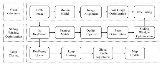
Figure 1.
System overview.
In the odometry thread, first, when the algorithm obtained a new stereo pair of images, a proposed forklift motion model predicted the current pose as the initial value for image alignment. The motion model was based on the assumption that the acceleration of the forklift remained constant for a short period so that the current pose could be predicted by the motion model of the forklift within this time frame [32]. Then, image alignment based on the direct method was implemented, and the relative poses of the current frame to the previous frame, as well as the current frame to the latest keyframe were obtained by minimizing the photometric error in the image pyramid. After the two step image alignment, the decision of whether to generate a new keyframe was made according to whether the current frame satisfied the requirements to be considered a keyframe. If the criteria for adding a new keyframe were satisfied, then the features were extracted on the basis of FAST corner and ORB description. However, in contrast to the method in ORB-SLAM, our approach used two step detection with a dynamic threshold for oriented multiscale FAST corners. The extraction speed was improved remarkably under the premise of ensuring uniform extraction. After that, feature matching between the new keyframe and the previous keyframe and outlier rejection based on circular matching were performed using the ORB description, and then, the pose of the new keyframe was updated using the remaining inlier matches. Conversely, if the conditions for adding a new keyframe were not met, then small pose graph optimization was implemented to optimize the pose from the current frame to the latest keyframe.
The sliding window optimization thread took the new keyframe and the matched features, which were the output of the odometry thread, and put them into the constant keyframe and map point set; then, a local bundle adjustment was performed on the keyframe. During the addition of the new keyframe and features, the keyframes that should be located in the window and those that should be completely deleted from the map or excluded from the optimization window were determined. Then, these unwanted keyframes were removed by marginalization during the optimization process.
The optional loop closing thread took the new features in the current keyframe from the odometry thread and checked whether the features in the current keyframe were similar to the features in historical keyframes. Once loop closure was detected, global bundle adjustment optimization was implemented, thus correcting the drift of the visual odometry and gaining global consistency.
3.1. Automatic Forklift
The robot for the designed SLAM algorithm was a manned electric forklift (model A30) produced by the HANGCHA company, as shown in Figure 2. The forklift was mounted on six pneumatic tires: four wheels at the front drove the machine, with every two fixed together, and two small wheels in the rear steered it. The total mass of the forklift was 4850 kg; the capacity of the lift was 1000 kg; and its velocity was limited up to 5 km/h for both empty and full load operations. The length, width, and height of the forklift were mm.
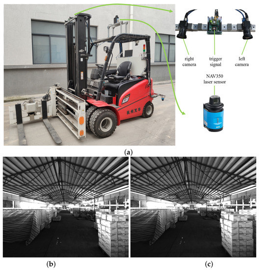
Figure 2.
The forklift equipped with basic sensors in our proposed system. (a) Two monocular cameras triggered by the same signal source are used to capture pictures of the warehouse, and the NAV350 sensor is used to measure the global position of the forklift in the warehouse. (b) The image captured by left the monocular camera; (c) the image captured by the right monocular camera.
Our SLAM algorithm was based on stereo pair images captured by two monocular cameras mounted in the forward facing direction on top of the lift. The two cameras were triggered by the same signal for picture synchronization. The ground truth came from the SICK NAV350 2D laser scanner navigation sensor attached at the top of the forklift. The forklift could operate in automatic mode or manual mode, which could be switched at any time. In order to obtain automatic navigation of the forklift, we designed a control system that controlled the steering wheel, accelerator signal, and lift signal with a computer and was equipped with the necessary sensors.
3.2. Basic Notations
3.2.1. Coordinate Transformation
The forklift pose can be represented by a transform matrix :
where is a transformation matrix from the current forklift coordinate system to the world coordinate system, with the relative rotation matrix and the translation vector . In particular, represents the special Euclidean group [33], defined as follows:
The 3D rotation matrix constitutes a special orthogonal group:
During the estimation of the relative transformation using optimization tools, the optimized relative pose can be estimated by minimizing the energy function. For that purpose, the Lie algebra [33] of corresponding to the tangent space of was used:
We denote the Lie algebra elements as , in which is translation and is 3D rotation. The meaning of ∧ is extended: ∧ acts on to convert a six-dimensional vector into a four-dimensional matrix. Each transformation matrix can be computed from using the exponential function according to Lie algebra:
For a point in the world coordinate system, we used to represent its homogeneous coordinate formation, so we could apply left multiplication of the transformation matrix to transform into in the current camera coordinate system:
For cases without ambiguity, could represent both the homogeneous and non-homogeneous coordinates.
3.2.2. Camera Projection
The grayscale image grabbed at time step i is denoted by . The measurement of a point in the camera oriented coordinate system can be represented by .
The pinhole camera model is a very common and effective model:
where represents the camera intrinsics and is generally considered to be a constant that is fixed after the camera is produced. can be obtained by calibration. It describes the 3D point-to-image projection relationship, with the projection function denoted by .
It is possible that the depth of the 3D point is lost after projection; on the contrary, if the depth Z corresponding to measurement is given, then the 3D point in the camera coordinate system can be computed by an inverse projection function :
4. Visual Odometry
4.1. Motion Model
In contrast to a UAV mounted or hand held camera, the pose of a camera that is equipped on a forklift corresponds to its kinematic constraints. Therefore, the motion of the camera can be estimated using the motion model of the forklift [34]. First, the kinematic model of the forklift is analyzed as described below.
The principle of the forklift robot with rear wheel steering is shown in Figure 3. and represent the world coordinate system and the forklift coordinate system, respectively.
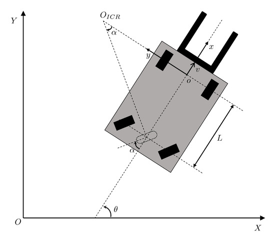
Figure 3.
Schema of the forklift with a spin-turn steering mechanism.
The angle between the rear wheel of the forklift and the y-axis of the forklift coordinate system is denoted by , and the counter-clockwise direction is positive. The velocity of the front drive shaft center of the forklift is defined as forklift speed v, and the angle between the longitudinal axis of the forklift coordinate system y and the world coordinate system Y is defined as the course angle of the forklift, which is denoted by , taking the counter-clockwise direction as positive. The distance between the front and rear wheels of the forklift is defined as L. It was assumed that the wheel will not slip, and the instantaneous rotation center of the forklift was the intersection point of the normal direction of the front and rear wheels. The movement of the forklift can easily be obtained in accordance with the following constraints:
This is the kinematic model of the wheeled vehicle, and it describes the relationship between the acceleration and motion of the vehicle. Because the camera and forklift were fixed to each other, the camera and the forklift could be regarded as a rigid body, so the motion of the camera accorded with the above kinematic constraints. The camera was mounted at the top center of lift, and its optical center coincided with the X-axis of the forklift. The distance between the lift and the Y-axis of the forklift was measured by a laser ruler, so the rigid transformation between them could be obtained. represents the camera’s pose in forklift coordinate, represents the forklift’s pose in the world coordinate, so the camera’s pose in world . Therefore, the motion model of the forklift could be used to roughly estimate the pose of the camera. The result of pose estimation could be used as the initial value of the direct method to solve the pose of the camera [32] to improve the speed of solving the pose of the camera, to reduce the time of the nonlinear optimization algorithm, and to reduce the probability that the direct method optimization falls into the local optimum. In general, the acceleration of a vehicle is relatively stable in the course of its operation and does not change dramatically as in the case of a hand held camera or a camera deployed on a UAV. The steering angle and speed v of the forklift truck cannot change instantaneously. The derivatives of these variables are the control signals of the vehicle.
This study assumed that the change rate of the forklift control signal remained unchanged within a short period; that is, the change in the control quantity in a certain period of time during the movement of the vehicle was linear.
The forklift’s pose at is . The coordinates and and the course angle of the forklift at can be solved from . The linear velocity of the vehicle is , and the angle of the wheel is at the time . Their control quantities are and , assuming that the error obeyed a Gaussian distribution with a zero mean and assuming they were independent of each other. The motion model of the vehicle was nonlinear and approximated by the first order Taylor series. The finite difference method was used to approximate the derivative of the forklift state variables.
Therefore, the approximate discrete time model of the system was established.
Next, we needed to find two states and . By solving the following least squares problem for N continuous frames, we could obtain the optimal estimates of and to calculate the line speed and wheel rotation angle of the vehicle at the next moment, which could be used to estimate the pose of the vehicle at the next moment:
4.2. Feature Detection
In the existing SLAM framework, the selection of points to track is related to the accuracy of camera pose estimation. In particular, in order to increase the accuracy of pose estimation, features that need to be extracted should be distributed as evenly as possible in the image. However, the location of feature point extraction depends heavily on the image itself, so it is difficult to make the features evenly distributed to the greatest extent possible.
For this reason, a two step feature extractor with a dynamic threshold was proposed, which could significantly improve the extraction efficiency. The detailed steps are shown in Algorithm 1.
| Algorithm 1: Two step dynamic threshold feature extraction. |
 |
In the first step, the initial threshold was used to extract the features from the whole image, and then, the threshold was modified according to the number of features extracted. If the number of features was lower than expected, then the texture of the image was not rich, so it was necessary to reduce the threshold and re-extract more features. When the threshold was reduced to a pre-set minimum value, the number of feature points to be extracted was insufficient, which indicated that this image was textureless and could only use the features already extracted. In our algorithm, the expected number of features was set to 1000, and the minimum threshold was set to seven. Feature points that were extracted by using an unrealistically small threshold were very unstable and had no application value. On the other hand, if the number of features was more than twice the expected value, then the image contained features in abundance, so we needed to extract stronger features as the object of tracking. However, because the appearance of the adjacent image was not very different, the system overhead could be reduced since the re-extraction of features of the current image was not necessary. Feature extraction of the subsequent image then used a modified threshold.
Moreover, after completing the overall extraction on the current image, the image was divided into cells, and then, the number of features in each cell was counted. If the number of features in a cell was lower than expected, then the threshold was reduced to re-extract the current cell until the number of features reached the target number or the threshold was reduced to the minimum. After processing all the cells, the quadtree model was used to screen all the features, and N features with a higher response value were obtained as an average as much as possible.
The two step feature extraction method could significantly reduce the number of calls of feature extraction functions. In the warehouse environment, the efficiency of two step extraction was much better than one step extraction, in which the image was divided into cells and features were extracted cell-to-cell. Further, the quality and distribution of feature points extracted were basically the same, as shown in Section 6.
4.3. Direct Image Alignment
After the pose of the forklift was estimated using the motion model, the algorithm grabbed a new stereo-pair frame, and only the left image was used in this step. First, the relative transformation of the current new frame against the last frame was computed. Further, because the latest keyframe may be updated, the relative transformation of the current new frame against the latest keyframe was then calculated to improve the accuracy of odometry. represents the current frame; reference frame represents the last frame or last keyframe; and the transformation between them is expressed as , which is denoted by in Lie algebra, given by:
where is the current frame pose estimated by the motion model and is the reference frame pose. For one keypoint with valid depth information in reference frame observed in the target current frame , given an initial relative transformation, was estimated by the motion model. According to the projection model of the camera, the keypoint observed in the current frame is:
Once is observed in the current frame, the photometric error of in reference and in current frame can be defined as:
where denotes a small neighborhood of pixels around keypoint . is the Huber norm. In particular, the slightly spread pattern proposed by DSO was used to achieve a trade-off between computational effort and accuracy. is the weight function based on the pixel gradient that is inversely proportional to it.
where cexpresses the constant gradient penalty factor. is the Euclidean norm. Thus, the optimized relative transformation can be computed by minimizing the full photometric error over the reference frame and the current frame [35].
where is all keypoints in the reference frame and denotes the photometric error mentioned earlier.
The above optimization process was carried out twice. The first step was to align the new frame and the previous frame to determine the current camera pose; the second step was to align the new frame and the last keyframe with the initial pose of the first step’s result and determine the final pose of the camera. Therefore, the reference frame could be set as keyframe or non-keyframe; the depth of the keypoint in the keyframe came from the sum of absolute difference (SAD) in the stereo pair in Section 4.4. When the reference frame was set to non-keyframe, the transformation between the reference and last keyframe was optimized, as well as the keypoint in the reference frame was associated with the corresponding keypoint in the last keyframe, so its coordinate in the reference frame could be calculated by transformation: . Although the first stage would be sufficient to estimate the camera pose, errors accumulated very easily, especially in the process of back-end optimization. The pose of the last keyframe may be updated, so it was very important to update the current frame camera pose in a timely manner according to the last keyframe. Two step sparse direct image alignment could improve the accuracy of the current frame pose, which was the main reason that the current frame was aligned with the last keyframe on the basis of the alignment with the previous frame.
The frames were downsampled to construct an image pyramid of eight levels and improve the efficiency of image alignment. Images were aligned at each pyramid level, beginning at the top of the pyramid and ending at the bottom. The results of each layer’s alignment were initial values for the next level of optimization, which dramatically reduced the number of iterations in the optimization process. To save optimization processing time, in the optimization process from top to bottom of the pyramid images, if the results converged, then several layers of images between them would be skipped, and the bottom layer images would align.
4.4. Feature Based Keyframe Refinement
Feature based methods of camera pose estimation can obtain good accuracy, but it is difficult to achieve high computational efficiency. Feature based methods need to extract features and match them for every single image, but there is much redundancy in the content of adjacent images, so this method was very inefficient. However, the hybrid method, which combined direct and indirect methods, used direct image alignment to obtain the pose of the camera in a non-keyframe, and when the distance between the last keyframe and the current frame was large enough, the keyframe was added to update the pose of the current keyframe by using the feature matching method, which significantly improved the computational efficiency.
After direct image alignment, the algorithm determined whether a new keyframe needed to be added. When the new keyframe was created, the FAST keypoints were extracted using the method described in Section 4.2, and then, the ORB descriptors were computed to match the features of the last keyframe. In our algorithm, because the current keyframe camera pose, which was close to the real pose, was obtained by direct image alignment, the matching process could be accelerated by the initial new keyframe camera pose. First, all the points visible in the last keyframe were projected in the new keyframe according to the initial pose of the new keyframe. Then, keypoints that were near the projection keypoint in the new keyframe were selected as the candidate points to match the projection point. The keypoint with the highest similarity was the matching point. Thus, the number of candidate keypoints was greatly reduced, so the computational cost remained small.
After using the ORB descriptor to match keypoints between the last left keyframe image and the new left keyframe image, the right keyframe image information was needed to obtain the depth of the keypoints in the new keyframe. For keypoints that were matched with the last keyframe, the initial depth could be obtained by projecting the points. Therefore, when searching for depth information, we could make full use of these initial depth values to accelerate the computation. According to the initial depth of the keypoint, the searching range of the corresponding position of the keypoint in the right image could be determined. Then, the sum of absolute difference (SAD) method was used to find the corresponding position of this keypoint in the right image. However, for a new keypoint extracted from the left image that did not match, SAD was used to find the corresponding match across the epipolar line in the right image.
Once the matching relationship of keypoints between the new keyframe and the last keyframe was obtained, the pose of the new keyframe could be optimized by minimizing the re-projection error of the keypoints from 3D to 2D:
where is the 3D point that can be seen in the last keyframe and the new keyframe at the same time and is the projection function of in the new current keyframe pose and is the Euclidean norm.
4.5. Outlier Rejection
Because of dynamic factors or repeated textures in the environment, there was a high probability of outlier points, which caused mismatching in the process of feature matching. Although numerous matched points were used in the optimization and a certain number of outliers could be tolerated, when the number of external points was large, the optimization accuracy was significantly reduced or the tracking was even lost. Therefore, it was necessary to remove as many outliers as possible while ensuring calculation efficiency.
Two efficient mechanisms were used by our algorithm to cull outliers.
First, after completing the ORB feature point matching, simplified loop chain matching was implemented to detect the quality of the matching. Specifically, the images of the last keyframe and the new keyframe are represented by , , , and , for which the superscripts L and R represent the left image and right image. For a point in , its corresponding position in is , and their correspondence was obtained by SAD based stereo image matching in the last calculation period. The point corresponds to the matching point in matched by the ORB descriptor; corresponds to the match point in obtained by SAD based stereo image matching. The calculation of the two parts was performed in the feature matching step mentioned above; therefore, when performing loop chain matching outlier detection, three of four sides of the loop chain were tested, and when four points were found by SAD, only normalized cross-correlation (NCC) would be used on a patch around and , and features with a low NCC score would be rejected.
Moreover, in the process of optimization iteration, the outliers were identified and then eliminated according to the reprojection error, as in the process for ORB-SLAM2.
5. Mapping
Visual odometry could estimate the camera pose in a short time by direct image alignment, feature matching, and the addition of keyframes and map points to the map at the same time. However, errors inevitably accumulated during the continuous addition of keyframes for map expansion, and the camera pose estimated by visual odometry became unreliable. Therefore, the back-end optimization of SLAM was required to reduce the error for keyframes and map points that were added to the map. Additionally, the 3D map of the warehouse environment needed to be established to meet the requirements for path planning and obstacle avoidance for the forklift operating in the warehouse. Therefore, a 3D grid map based on an octree was constructed according to the point cloud map [36]. The example of the point cloud map and the grid map is shown in Section 6.4.
5.1. Keyframe Management
Our algorithm was based on sparse direct image alignment of the current frame to the last frame and the current to the last keyframe. As the camera moved, the content of the current frame changed constantly, and the keypoints that were tracked from the last keyframe were significantly reduced, so it was necessary to add the keyframe to the map in time to guarantee the stability of visual odometry. Each frame was regarded as a candidate keyframe after image alignment, and whether the current frame was added to the map as a new keyframe was determined by applying several criteria:
- Enough time t (e.g., 1 s) had passed since the last keyframe was added;
- The number of keypoints in the last keyframe that were observed in the current frame was reduced by 30%.
- The distance or rotation of the current frame to the last keyframe exceeded the set threshold.
The first case applied to situations in which the camera was moving at a lower speed, and the latest information from the environment was added to the map to cope with dynamic factors in the environment. The second and third rules dealt with the camera moving at a faster speed by expanding the map in time to prevent the loss of localization.
It could be seen from the above that the conditions for adding keyframes were loose, so many keyframes were added to the map over time. However, because of limited memory capacity and computing power, redundancy and low quality keyframes must be culled. For example, when the camera was stationary, a large number of keyframes with almost the same appearance was added to the map, which was detrimental to the optimization process, resulting in the degradation of the optimization problem. If the number of keypoints of the common view in the two keyframes exceeded 90%, the keyframe added first was removed.
The above keyframe management strategy that added a keyframe to the map loosely and culled it from the map strictly was very effective. The loose keyframe selection strategy could expand the map in time, provide more landmark points for the map, and improve the stability of camera pose tracking. The strict culling mechanism of redundant keyframes ensured that the optimization did not degenerate while ensuring the system’s computational efficiency and low memory usage.
5.2. Map Optimization
In the framework of visual SLAM based on graph optimization, bundle adjustment played a central role. Because it could significantly reduce the error accumulated by visual odometry and had good real-time performance, it became a common practice of feature based SLAM. There are currently excellent open source programs for solving BA problems, such as Ceres and g2o. As in ORB-SLAM, our approach used g2o to optimize keyframes and 3D points on the map.
After a new keyframe was added to the map, BA was implemented; however, only some keyframes and map points were selected for local BA optimization in order to improve the efficiency of the optimization. Specifically, some of the keyframes newly added to the map, the keyframes that had a strong co-view relationship with them, and the 3D points that could be observed by these keyframes were selected as optimization targets. The keyframes and map points were optimized by minimizing the set errors of these 3D points in these keyframe projections and 2D observation points. The energy equation is:
where is the pose of the keyframe expressed in the Lie algebra form, represents a 3D point on the map, and is the observation value of the camera for the 3D point at the pose .
5.3. Loop Closure
Incremental frame tracking could cause drift accumulation, and after a small drift was transmitted through many keyframes, it could produce unacceptable results. Loop closure and global optimization were considered effective methods to solve this cumulative drift. The bag of binary words (BoW) [37] was applied for loop closure detection in the proposed approach. Loop closure detection was carried out after the new keyframe was added to the map. Once the loop was detected, the global BA was implemented to achieve the global consistency of the map.
6. Experimental Results and Discussion
Because our algorithm needed to be applied in the warehouse environment, some datasets were captured in a typical warehouse, and the results were summarized and analyzed in order to evaluate the efficiency and accuracy of our proposed stereo SLAM algorithm. Our results were mainly compared with ORB-SLAM2, which had balanced performance in all aspects. Open Source Computer Vision Library (OpenCV) was used in our algorithm to realize basic image processing. Both algorithms were run on a desktop PC with Intel Core I7-7700 CPU @ 3.6–4.2 GHz and 8 GB RAM. The desktop PC ran the Ubuntu 18.04 64 bit system.
6.1. Dataset
The dataset was recorded from the automatic forklift platform in a classic warehouse. Two identical grayscale cameras were used to capture the images. The specific model and parameters were as follows: FLIR Flea3 FL3-U3-13E4M-C mono camera, 1.3 megapixels, 1/1.8” e2v EV76C560 CMOS, global shutter, and maximum resolution 1280 × 1024; each camera was equipped with a Kowa lens with a 5 mm focal length, F2.8-F16, and angle of view. The baseline of the two cameras was set to 30 cm. The left and right cameras were triggered by the same source generated by STM32F103 MCU in order to synchronize their images, and the image acquisition frequency was set to 20 Hz.
The ground truth of the forklift needed to be recorded to evaluate the performance of the SLAM algorithm. The general practice was to use a motion capture system such as VICON to obtain the motion truth of the robot through external cameras and achieve high accuracy. However, the deployment of a motion capture system in a typical warehouse is very expensive because of its large area. In contrast to a UAV, the forklift only moved on the ground, so its position and heading could be used to describe the ground truth of the forklift. SICK LiDAR was deployed on top of the forklift to obtain the ground truth of the forklift by measuring a reflective landmark that was pre-arranged in the warehouse. The LiDAR model was NAV350; the scanning frequency was 8 Hz; and the scanning angle was . The cameras and SICK LiDAR are shown in Figure 4.
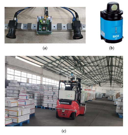
Figure 4.
Dataset collection platform that includes the stereo camera, NAV350 laser sensor, artificial reflective landmark, and automatic guided forklift. (a) Stereo camera. Two monocular cameras triggered by the same signal source were used to capture pictures of the warehouse. (b) SICK NAV350. The NAV350 sensor was used to measure the global position of the forklift in the warehouse. (c) The forklift running in the warehouse.
The cameras were connected to the PC through USB 3.0 interfaces, and the LiDAR was connected to the PC through a Gigabit Ethernet interface run at 100 megabits. The recording PC ran on Intel I5 6200U, 8 GB RAM, and 256 GB SSD. The PC ran the Ubuntu 18.04 64 bit system. In order to prevent frame loss and ensure complete data recording, we used optimized multithreading to process each camera and the LiDAR, respectively. The grayscale images were stored in the 8 bit PNG image format, and the ground truth recorded by LiDAR was recorded in a TXT file.
Because the wide angle lens was used, it was necessary to calibrate the cameras. After the dataset collection, the radial distortion and stereo rectification were implemented. Sample rectified images from the dataset are shown in Figure 5. This was a challenging dataset since its area was significantly larger than that of an ordinary indoor scene: the length of the warehouse was 100 m, and the width is 30 m. Meanwhile, the warehouse had dynamic illumination, long corridors, and repetitive scenes.
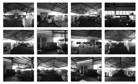
Figure 5.
Sample images from the warehouse dataset, which contains the typical scene in the warehouse and these images from the left camera.
6.2. Efficiency Experiment
6.2.1. Feature Detection Performance
First, our two step dynamic threshold feature extraction was compared with the feature extraction carried out by ORB-SLAM on the warehouse dataset. The parameter settings of the two feature extraction algorithms were the same. The number of expected features was 2000; the image was divided into 10 × 10 cells; the initial threshold was set to 20; and the minimum threshold was set to 7.
Figure 6 shows the feature extraction execution time of every frame using our algorithm and ORB-SLAM on the warehouse dataset. It can be seen from the figure that our algorithm execution time was significantly less than the feature extraction time of ORB-SLAM, and the operation was very stable. Furthermore, changing the scene had little effect on the running time of our algorithm, whereas it greatly affected the running time of the feature extraction algorithm in ORB-SLAM. A constant feature extraction time was necessary for constant tracking speed. Therefore, our algorithm was superior to the feature extraction algorithm in ORB-SLAM in terms of extraction speed and running stability.
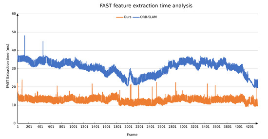
Figure 6.
Time analysis of two different feature extraction algorithms on each image in the warehouse dataset.
Figure 7 and Table 1 show the performance of the two feature extraction algorithms after reducing the number of desired features. When the number of expected features was reduced from 2000 to 500 in decrements of 500, our algorithm execution time was reduced by , , and , respectively. However, the execution time of the feature extraction algorithm in ORB-SLAM was only reduced by , , and , respectively. The reason for the relatively low effect on ORB-SLAM was that it must extract features from each cell regardless of whether the texture in the current frame was rich; thus, the overhead of the algorithm was constant irrespective of the number of desired features. However, our algorithm extracted enough features in the first overall extraction step, and it only re-extracted from cells with less texture. Therefore, when the number of desired feature points was reduced, our algorithm runtime significantly decreased.
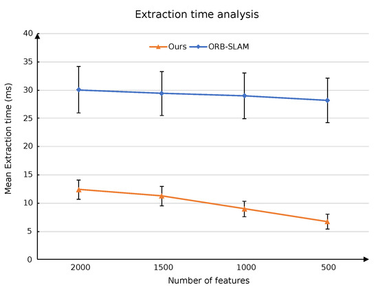
Figure 7.
The effect of different numbers of expected feature points on the efficiency of two feature extraction algorithms.

Table 1.
Comparison of extraction times.
Figure 8 shows that the two different feature extraction algorithms extracted fast feature points from the same frame and obtained almost the same results. This was because, although the logic of the algorithm was different, the fast feature point extraction function of OpenCV was called at the bottom.
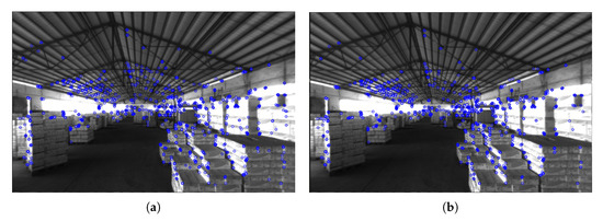
Figure 8.
Feature extraction results of the same image by two feature extraction algorithms. (a) The proposed two step dynamic threshold feature extraction. (b) The method that divides the image into cells and extracts features in each cell.
6.2.2. Tracking Efficiency
The computational efficiency of our algorithm was evaluated by a statistical analysis of the tracking time of each frame using the warehouse dataset. The performance of ORB-SLAM2 on this dataset was also evaluated. The number of tracking keypoints of both algorithms was set to 2000.
As shown in Figure 9 and Table 2, our algorithm only required 17 ms to track a new frame. The fastest time used to track a new frame using the direct method was 6.53 ms. The worst result using the feature matching method was still less than 100 ms. Therefore, our algorithm could be easily run in real time using a normal CPU core. In contrast, ORB-SLAM required an average of more than 100 ms to track a new frame, and the worst case was 288 ms. Obviously, ORB-SLAM was difficult to run in real time on our dataset.
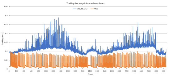
Figure 9.
Comparison of tracking performances between our algorithm and ORB-SLAM2. The peak in our tracking time corresponds to the addition of keyframes, which need more time to extract features and match them, update the depth of keypoints, and optimize camera pose.
Table 2.
Time statistics for the detection of 2000 keypoints in the dataset.
The remarkable improvement in the efficiency of our algorithm was attributed to three main reasons. First, ORB-SLAM extracted and matched keypoints for each frame, whereas our algorithm used image alignment to track each frame and then only extracted and matched keypoints for keyframes. Because the number of keyframes was far less than all frames, image alignment could be realized with a very fast calculation speed as a result of its linear calculation complexity. Thus, our hybrid method could significantly improve the calculation efficiency. Second, we adopted the above discussed two step dynamic threshold feature extraction method, so the feature extraction time (the most time consuming step of tracking) was greatly reduced while ensuring the uniform distribution of feature points. Finally, the pose estimation based on the forklift motion model could provide a more reasonable initial value for the new frame, thereby reducing the number of calculation iterations.
6.3. Accuracy Experiment
The experimental accuracy of our algorithm was evaluated using the warehouse environment. As a reference, the result of the SICK NAV350 2D laser navigation system was taken as the ground truth trajectory, as shown in Figure 10. In addition, a state-of-the-art method was compared with our algorithm. Accuracy was compared by computing the absolute translation root mean squared error (RMSE) between the trajectory of the SLAM result and the ground truth. Each algorithm was run five times on multiple sequences, and the average RMSE was taken as the final result. We plotted the trajectories of the localization results of our algorithm and ORB-SLAM2, as well as the trajectories of the ground truth obtained by the laser navigation system. It can be seen that both methods achieved high localization accuracy.
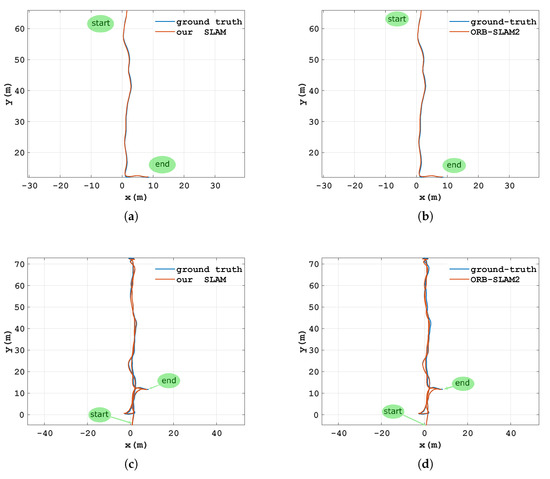
Figure 10.
Accuracy performance of our method and ORB-SLAM2 for different sequences using a laser sensor as the ground truth. (a) Ours-a. (b) ORB-SLAM2-a. (c) Ours-b. (d) ORB-SLAM2-b.
Table 3 shows the accuracy performance on the warehouse dataset of our method and ORB-SLAM2. The RMSE results for our system are provided in Table 3. In addition, our method was compared with the state-of-the-art approach ORB-SLAM2. The table lists RMSE values of the absolute trajectory error for the two methods, and our method achieved comparable accuracy to ORB-SLAM2 and even exceeded its accuracy for some sequences. It should be noted that this high accuracy was achieved by our method while greatly reducing the tracking time because of the hybrid tracking model and the kinematic model of the forklift in Section 4.
Table 3.
Accuracy performance on the warehouse dataset.
6.4. Mapping Result
Figure 11 shows the results of mapping. Our SLAM solution used a stereo camera, which could obtain the scale of the points. The point cloud map showed that our method accurately constructed the structure of the warehouse, with very few outliers added to the map. Then, from the point cloud map, the octree map was generated to provide a basis for subsequent path planning and obstacle avoidance. The point clouds exceeding the specified height would not affect path planning and obstacle avoidance; only point clouds within the specified height range were selected to generate the octree map.
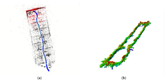
Figure 11.
3D point cloud map and octree map created for the warehouse. (a) Point cloud map; points in red color represent the keypoints in current optimization window; black represents the optimized keypoints; blue represents keyframes; and green is the edge between keyframes. (b) Octree map; the different color was set according to the height of voxels.
7. Conclusions
In this paper, we presented a stereo visual SLAM approach for a forklift operating in a large scale indoor warehouse. Experimental results showed that our method had impressive efficiency and high accuracy. The hybrid tracking model took advantage of the high efficiency of the direct method and the high precision of the indirect method. For a new frame, direct image alignment was applied to obtain its pose, and then, feature extraction and matching were implemented to update the pose of the keyframe, thereby achieving a balance between efficiency and accuracy.
In the front-end of SLAM, visual odometry, we proposed a two stage dynamic threshold feature extraction method, which could significantly decrease the time required for feature extraction while maintaining the same quality of the keypoints. In addition, since the SLAM applied to a vehicle differed from that used for a hand held camera, the motion of the camera was constrained by the kinematics of the vehicle: therefore, a kinematic model of the forklift was constructed to provide a more reasonable initial position and pose value for the direct method and further increase the speed of optimization convergence.
Compared with the indirect method, given the same parameters, our algorithm significantly improved the tracking efficiency on a dataset of a warehouse, and the accuracies of the two methods were comparable. Our method has great potential to be transplanted to embedded computers, such as Intel Upboard or Raspberry Pi 4.
Although the proposed method achieved high computational efficiency and accuracy, there are still many improvements to explore in the future. First, compared with the current indirect estimation of the vehicle motion state through pose, wheel odometry can calculate the trajectory of a vehicle accurately in a short time; moreover, IMUs can measure vehicle acceleration and angular velocity more directly, and integrating IMUs or wheel odometry data can increase the robustness of pose tracking. Then, the vehicle control and SLAM process can be combined to develop an active SLAM algorithm to enhance the adaptability of the algorithm to the environment.
Author Contributions
H.L. designed the entire core architecture. F.W. performed the algorithm and wrote the paper. E.L. supervised the research. Y.W. reviewed and edited the manuscript. G.Q. analyzed the data. All authors read and agreed to the published version of the manuscript.
Funding
This research was supported, in part, by the Natural Science Fund of China (Project No. 31971806 and No. 51705161), the Sub-task of the National Key Research and Development Plan of China (Project No. 2018YFD0701002), the Sub-task of the National Science and Technology Support Plan of China (Project No. 2015BAD18B0301), and the Key Research and Development Plan of Guangdong (Project No. 2019B020225001).
Acknowledgments
We are thankful to Guangdong Tianhe Storage Co., Ltd, for providing the test scenario. The authors also thank the anonymous reviewers for their critical comments and suggestions to improve the manuscript.
Conflicts of Interest
The authors declare no conflict of interest.
References
- Roldán, J.J.; Peña-Tapia, E.; Garcia-Aunon, P.; Del Cerro, J.; Barrientos, A. Bringing adaptive & immersive interfaces to real-world multi-robot scenarios: Application to surveillance and intervention in infrastructures. IEEE Access 2019, 7, 86319–86335. [Google Scholar]
- Musić, J.; Kružić, S.; Stančić, I.; Papić, V. Adaptive Fuzzy Mediation for Multimodal Control of Mobile Robots in Navigation-Based Tasks. Int. J. Comput. Intell. Syst. 2019, 12, 1197–1211. [Google Scholar] [CrossRef]
- Walter, M.R.; Antone, M.; Chuangsuwanich, E.; Correa, A.; Davis, R.; Fletcher, L.; Frazzoli, E.; Friedman, Y.; Glass, J.; How, J.P.; et al. A Situationally Aware Voice-commandable Robotic Forklift Working Alongside People in Unstructured Outdoor Environments. J. Field Robot. 2015, 32, 590–628. [Google Scholar] [CrossRef]
- Pradalier, C.; Tews, A.; Roberts, J. Vision based operations of a large industrial vehicle: Autonomous hot metal carrier. J. Field Robot. 2008, 25, 243–267. [Google Scholar] [CrossRef]
- Cadena, C.; Carlone, L.; Carrillo, H.; Latif, Y.; Scaramuzza, D.; Neira, J.; Reid, I.; Leonard, J.J. Past, present, and future of simultaneous localization and mapping: Toward the robust-perception age. IEEE Trans. Robot. 2016, 32, 1309–1332. [Google Scholar] [CrossRef]
- Huang, B.; Zhao, J.; Liu, J. A Survey of Simultaneous Localization and Mapping. arXiv 2019, arXiv:1909.05214. [Google Scholar]
- Beinschob, P.; Reinke, C. Graph SLAM based mapping for AGV localization in large-scale warehouses. In Proceedings of the 2015 IEEE International Conference on Intelligent Computer Communication and Processing (ICCP), Cluj-Napoca, Romania, 3–5 September 2015; IEEE: Hoboken, NJ, USA, 2015; pp. 245–248. [Google Scholar]
- Chen, Y.; Wu, Y.; Xing, H. A complete solution for AGV SLAM integrated with navigation in modern warehouse environment. In Proceedings of the 2017 Chinese Automation Congress (CAC), Jinan, China, 20–22 October 2017; IEEE: Hoboken, NJ, USA, 2017; pp. 6418–6423. [Google Scholar]
- De Gaetani, C.; Pagliari, D.; Realini, E.; Reguzzoni, M.; Rossi, L.; Pinto, L. Improving Low-Cost GNSS Navigation in Urban Areas by Integrating a Kinect Device. In International Symposium on Advancing Geodesy in a Changing World, Proceedings of the IAG Scientific Assembly, Kobe, Japan, 30 July–4 August 2017; Springer: Cham, Switzerland, 2018; pp. 183–189. [Google Scholar]
- Wang, L.; Wu, Z. RGB-D SLAM with Manhattan Frame Estimation Using Orientation Relevance. Sensors 2019, 19, 1050. [Google Scholar] [CrossRef]
- Mu, X.; Chen, J.; Zhou, Z.; Leng, Z.; Fan, L. Accurate Initial State Estimation in a Monocular Visual–Inertial SLAM System. Sensors 2018, 18, 506. [Google Scholar]
- Bloesch, M.; Burri, M.; Omari, S.; Hutter, M.; Siegwart, R. Iterated extended Kalman filter based visual-inertial odometry using direct photometric feedback. Int. J. Robot. Res. 2017, 36, 1053–1072. [Google Scholar] [CrossRef]
- Cvišic, I.; Cesic, J.; Markovic, I.; Petrovic, I. Soft-slam: Computationally efficient stereo visual slam for autonomous uavs. J. Field Robot. 2017, 35. [Google Scholar] [CrossRef]
- Lowe, D.G. Object recognition from local scale-invariant features. In Proceedings of the Seventh IEEE International Conference on Computer Vision, Kerkyra, Greece, 20–27 September 1999; IEEE: Hoboken, NJ, USA, 2019; Volume 99, pp. 1150–1157. [Google Scholar]
- Bay, H.; Tuytelaars, T.; van Gool, L. Surf: Speeded up robust features. In European Conference on Computer Vision; Springer: Cham, Switzerland, 2006; pp. 404–417. [Google Scholar]
- Rublee, E.; Rabaud, V.; Konolige, K.; Bradski, G.R. ORB: An efficient alternative to SIFT or SURF. In Proceedings of the IEEE International Conference on Computer Vision, ICCV 2011, Barcelona, Spain, 6–13 November 2011. [Google Scholar]
- Hartley, R.I. In defense of the eight-point algorithm. IEEE Trans. Pattern Anal. Mach. Intell. 1997, 19, 580–593. [Google Scholar] [CrossRef]
- Longuet-Higgins, H.C. A computer algorithm for reconstructing a scene from two projections. Nature 1981, 293, 133. [Google Scholar] [CrossRef]
- Li, H.; Hartley, R. Five-point motion estimation made easy. In Proceedings of the 18th International Conference on Pattern Recognition, Hong Kong, China, 20–24 August 2006; IEEE: Hoboken, NJ, USA, 2006; Volume 1, pp. 630–633. [Google Scholar]
- Nistér, D. An efficient solution to the five-point relative pose problem. IEEE Trans. Pattern Anal. Mach. Intell. 2004, 26, 756–777. [Google Scholar] [CrossRef] [PubMed]
- Davison, A.J.; Reid, I.D.; Molton, N.D.; Stasse, O. MonoSLAM: Real-time single camera SLAM. IEEE Trans. Pattern Anal. Mach. Intell. 2007, 1052–1067. [Google Scholar] [CrossRef]
- Klein, G.; Murray, D. Parallel tracking and mapping for small AR workspaces. In Proceedings of the 6th IEEE and ACM International Symposium on Mixed and Augmented Reality, Nara, Japan, 13–16 November 2007; IEEE Computer Society: Washington, DC, USA, 2007; pp. 1–10. [Google Scholar]
- Mur-Artal, R.; Montiel, J.M.M.; Tardos, J.D. ORB-SLAM: A versatile and accurate monocular SLAM system. IEEE Trans. Robot. 2015, 31, 1147–1163. [Google Scholar] [CrossRef]
- Mur-Artal, R.; Tardós, J.D. Orb-slam2: An open-source slam system for monocular, stereo, and rgb-d cameras. IEEE Trans. Robot. 2017, 33, 1255–1262. [Google Scholar] [CrossRef]
- Kümmerle, R.; Grisetti, G.; Strasdat, H.; Konolige, K.; Burgard, W. G2o: A general framework for graph optimization. In Proceedings of the IEEE International Conference on Robotics and Automation, Shanghai, China, 9–13 May 2011; IEEE: Hoboken, NJ, USA, 2011; pp. 3607–3613. [Google Scholar]
- Engel, J.; Schöps, T.; Cremers, D. LSD-SLAM: Large-scale direct monocular SLAM. In Proceedings of the 13th European Conference on Computer Vision, Zurich, Switzerland, 6–12 September 2014; Springer: Cham, Switzerland, 2014; pp. 834–849. [Google Scholar]
- Glover, A.; Maddern, W.; Warren, M.; Reid, S.; Milford, M.; Wyeth, G. OpenFABMAP: An open source toolbox for appearance based loop closure detection. In Proceedings of the IEEE International Conference on Robotics and Automation, Saint Paul, MN, USA, 14–18 May 2012; IEEE: Hoboken, NJ, USA, 2012; pp. 4730–4735. [Google Scholar]
- Engel, J.; Stückler, J.; Cremers, D. Large-scale direct SLAM with stereo cameras. In Proceedings of the 2015 IEEE/RSJ International Conference on Intelligent Robots and Systems (IROS), Hamburg, Germany, 28 September–2 October 2015; IEEE: Hoboken, NJ, USA, 2015; pp. 1935–1942. [Google Scholar]
- Engel, J.; Koltun, V.; Cremers, D. Direct sparse odometry. IEEE Trans. Pattern Anal. Mach. Intell. 2017, 40, 611–625. [Google Scholar] [CrossRef]
- Wang, R.; Schworer, M.; Cremers, D. Stereo DSO: Large-scale direct sparse visual odometry with stereo cameras. In Proceedings of the IEEE International Conference on Computer Vision, Venice, Italy, 22–29 October 2017; pp. 3903–3911. [Google Scholar]
- Engel, J.; Usenko, V.; Cremers, D. A photometrically calibrated benchmark for monocular visual odometry. arXiv 2016, arXiv:1607.02555. [Google Scholar]
- Persson, M.; Piccini, T.; Felsberg, M.; Mester, R. Robust stereo visual odometry from monocular techniques. In Proceedings of the IEEE Intelligent Vehicles Symposium (IV), Seoul, Korea, 28 June–1 July 2015; IEEE: Hoboken, NJ, USA, 2015; pp. 686–691. [Google Scholar]
- Selig, J.M. Lie groups and lie algebras in robotics. In Computational Noncommutative Algebra and Applications; Springer: Haarlem, The Netherlands, 2004; pp. 101–125. [Google Scholar]
- Tamba, T.A.; Hong, B.; Hong, K.S. A path following control of an unmanned autonomous forklift. Int. J. Control Autom. Syst. 2009, 7, 113–122. [Google Scholar] [CrossRef]
- Forster, C.; Pizzoli, M.; Scaramuzza, D. SVO: Fast semi-direct monocular visual odometry. In Proceedings of the IEEE International Conference on Robotics and Automation (ICRA), Hong Kong, China, 31 May–7 June 2014; pp. 15–22. [Google Scholar]
- Hornung, A.; Wurm, K.M.; Bennewitz, M.; Stachniss, C.; Burgard, W. OctoMap: An efficient probabilistic 3D mapping framework based on octrees. Auton. Robot. 2013, 34, 189–206. [Google Scholar] [CrossRef]
- Gálvez-López, D.; Tardos, J.D. Bags of binary words for fast place recognition in image sequences. IEEE Trans. Robot. 2012, 28, 1188–1197. [Google Scholar] [CrossRef]


© 2020 by the authors. Licensee MDPI, Basel, Switzerland. This article is an open access article distributed under the terms and conditions of the Creative Commons Attribution (CC BY) license (http://creativecommons.org/licenses/by/4.0/).