On the Statistical Significance of the Variability Minima of the Order Parameter of Seismicity by Means of Event Coincidence Analysis


Abstract
:1. Introduction
2. Methods
2.1. Natural Time Analysis
2.2. Event Coincidence Analysis
3. Results
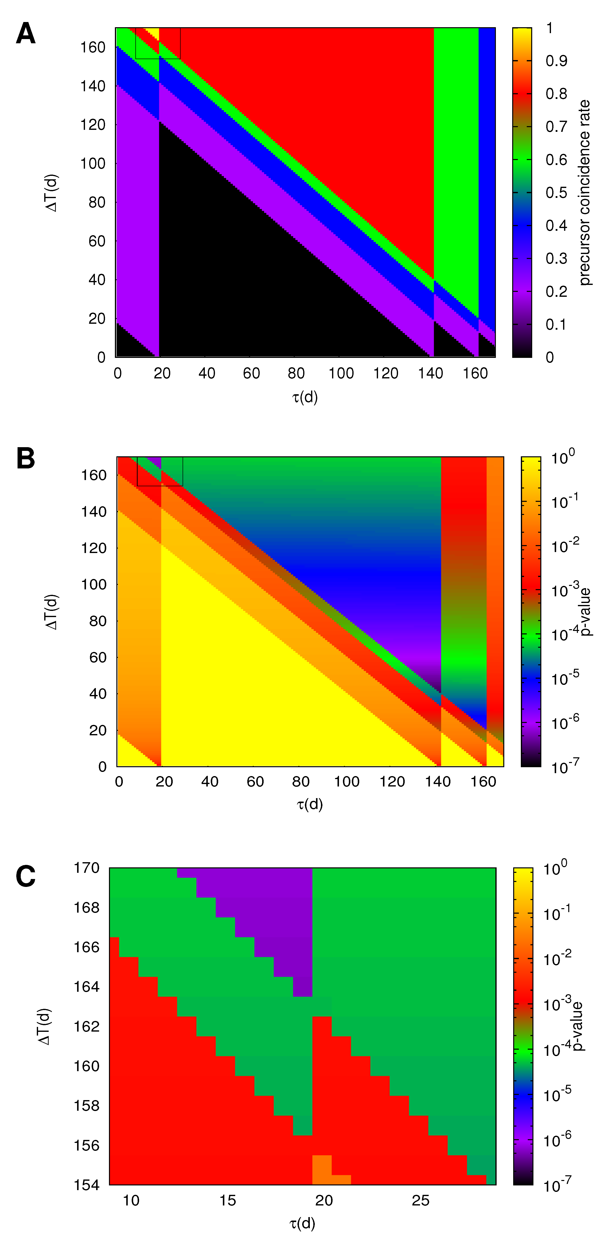
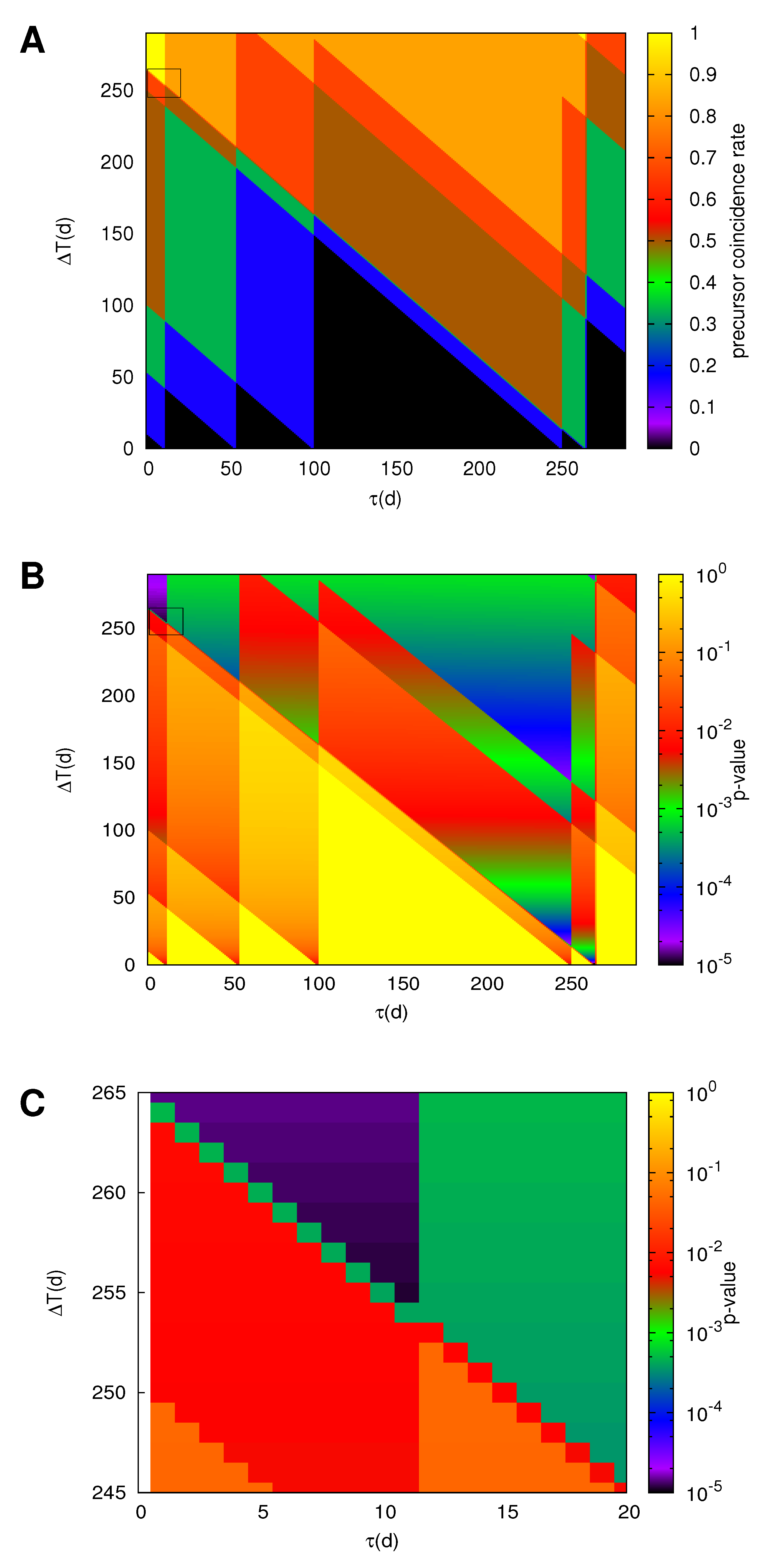
3.1. Japan
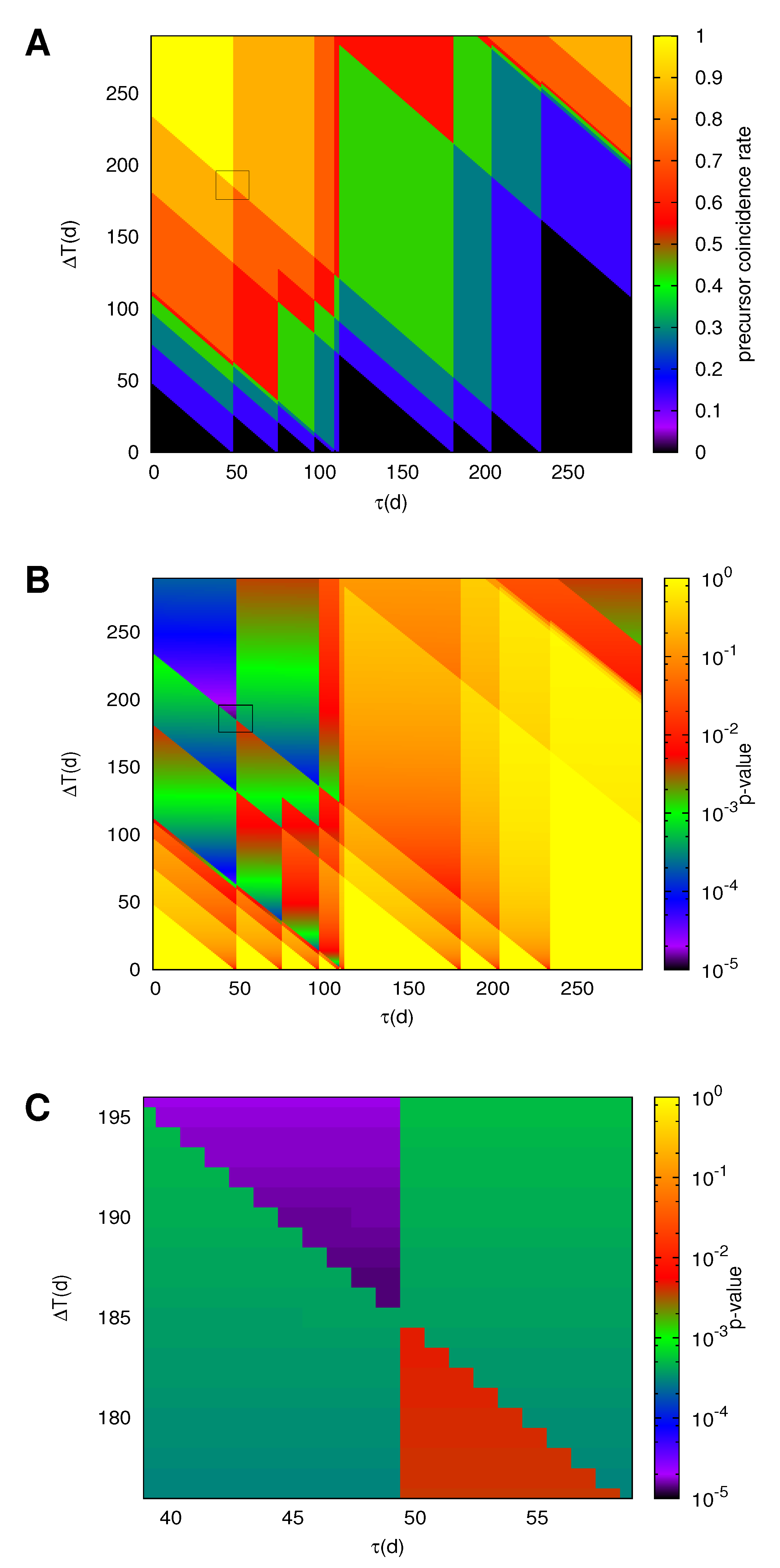
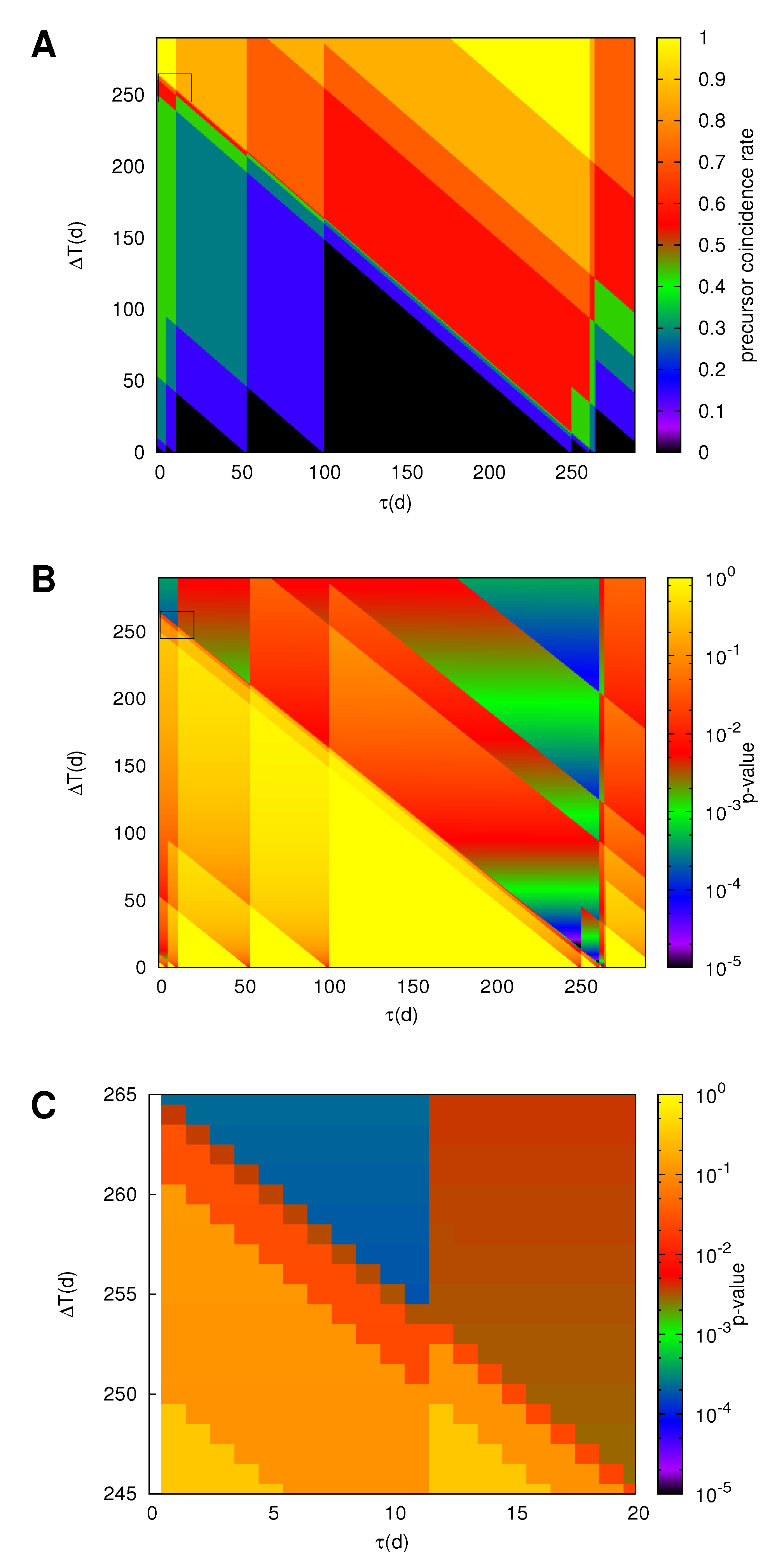
3.2. Eastern Mediterranean
3.3. Global Seismicity
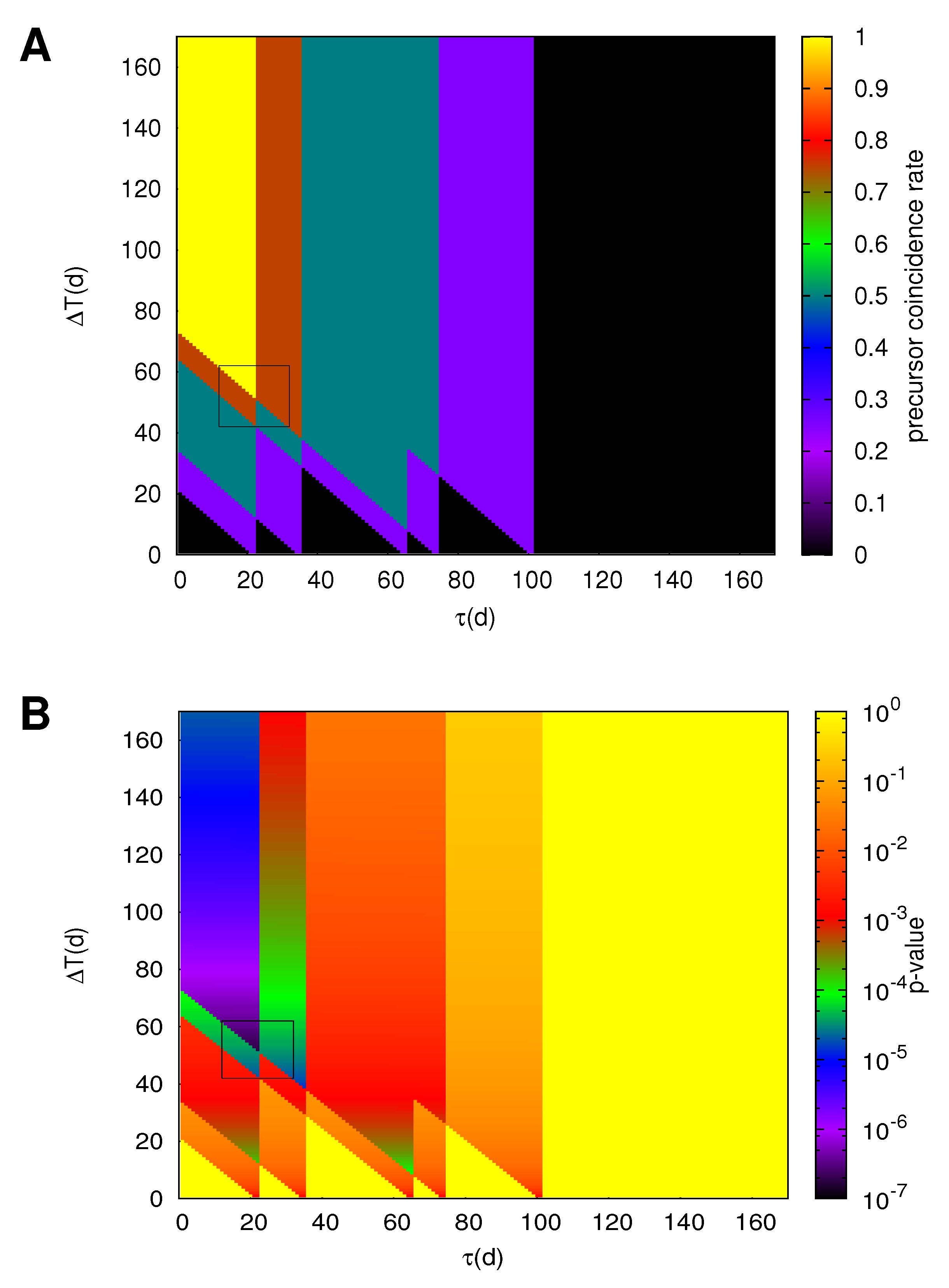
3.3.1. Focusing on EQs with M
3.3.2. Focusing on EQs with M
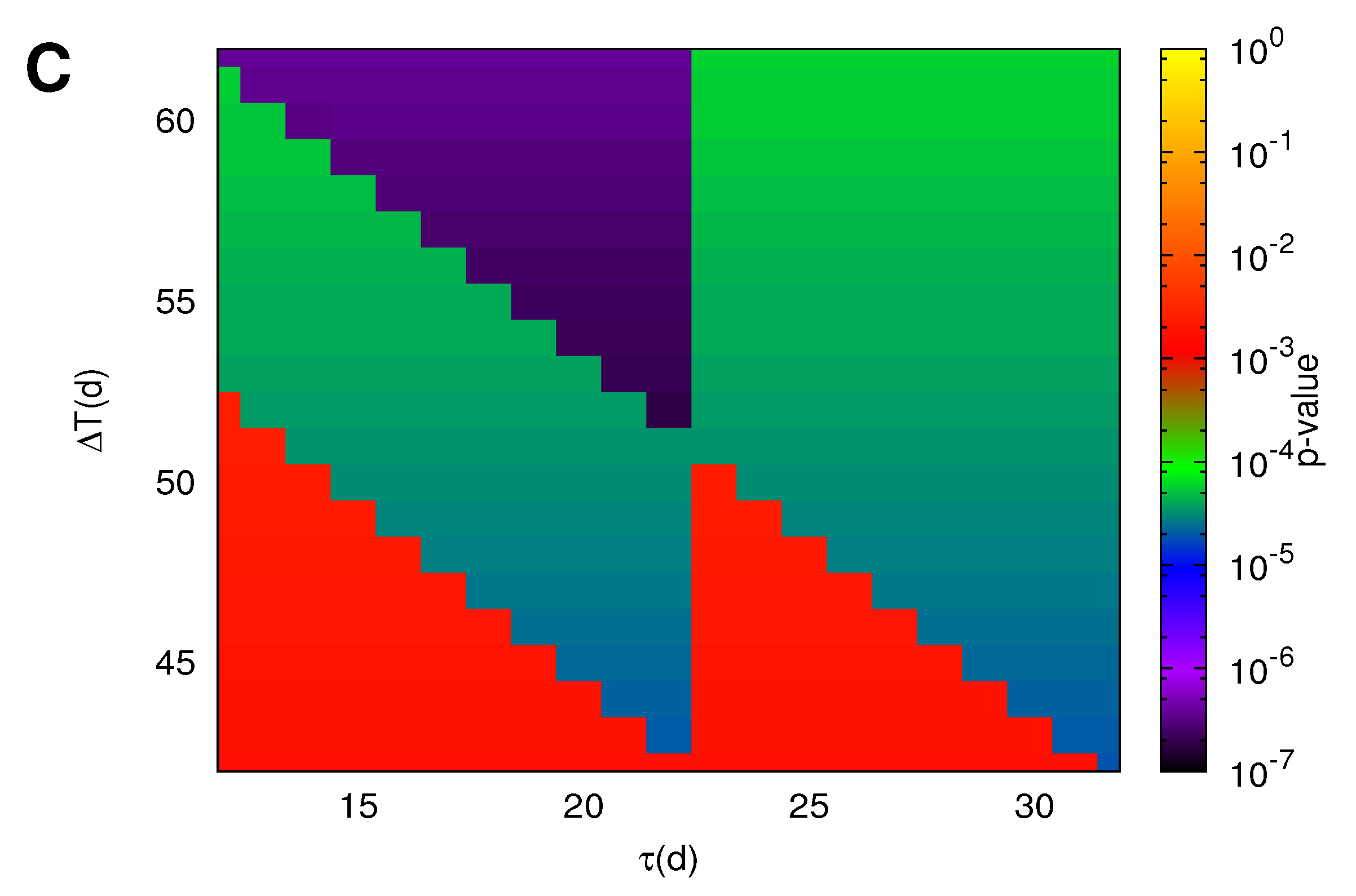
3.3.3. Focusing on EQs with M and Using Mid-Scale Seismicity
4. Discussion
5. Conclusions
Author Contributions
Funding
Conflicts of Interest
Abbreviations
| ECA | Event coincidence analysis |
| ENBOSAP | Earthquake networks based on similar activity patterns |
| EQ | Earthquake |
| FA | False alarm |
| JMA | Japan Meteorological Agency |
| NTA | Natural time analysis |
| SES | Seismic electric signals |
References
- Donges, J.; Schleussner, C.F.; Siegmund, J.; Donner, R. Event coincidence analysis for quantifying statistical interrelationships between event time series. Eur. Phys. J. Spec. Top. 2016, 225, 471–487. [Google Scholar] [CrossRef] [Green Version]
- Hassanibesheli, F.; Donner, R.V. Network inference from the timing of events in coupled dynamical systems. Chaos Interdiscip. J. Nonlinear Sci. 2019, 29, 083125. [Google Scholar] [CrossRef] [PubMed]
- Siegmund, J.F.; Siegmund, N.; Donner, R.V. CoinCalc—A new R package for quantifying simultaneities of event series. Comput. Geosci. 2017, 98, 64–72. [Google Scholar] [CrossRef] [Green Version]
- Schleussner, C.F.; Donges, J.F.; Donner, R.V.; Schellnhuber, H.J. Armed-conflict risks enhanced by climate-related disasters in ethnically fractionalized countries. Proc. Natl. Acad. Sci. USA 2016, 113, 9216–9221. [Google Scholar] [CrossRef] [PubMed] [Green Version]
- Sun, A.; Scanlon, B.; AghaKouchak, A.; Zhang, Z. Using GRACE Satellite Gravimetry for Assessing Large-Scale Hydrologic Extremes. Remote. Sens. 2017, 9, 1287. [Google Scholar] [CrossRef] [Green Version]
- Sun, A.Y.; Xia, Y.; Caldwell, T.G.; Hao, Z. Patterns of precipitation and soil moisture extremes in Texas, US: A complex network analysis. Adv. Water Resour. 2018, 112, 203–213. [Google Scholar] [CrossRef]
- Sarlis, N.V. Statistical Significance of Earth’s Electric and Magnetic Field Variations Preceding Earthquakes in Greece and Japan Revisited. Entropy 2018, 20, 561. [Google Scholar] [CrossRef] [Green Version]
- Varotsos, P.A.; Sarlis, N.V.; Skordas, E.S. Natural time analysis: Important changes of the order parameter of seismicity preceding the 2011 M9 Tohoku earthquake in Japan. EPL (Europhys. Lett.) 2019, 125, 69001. [Google Scholar] [CrossRef] [Green Version]
- Varotsos, P.A.; Sarlis, N.V.; Skordas, E.S. Spatio-Temporal complexity aspects on the interrelation between Seismic Electric Signals and Seismicity. Pract. Athens Acad. 2001, 76, 294–321. [Google Scholar]
- Varotsos, P.A.; Sarlis, N.V.; Skordas, E.S. Long-range correlations in the electric signals that precede rupture. Phys. Rev. 2002, 66, 011902. [Google Scholar] [CrossRef] [Green Version]
- Varotsos, P.A.; Sarlis, N.V.; Skordas, E.S. Natural Time Analysis: The New View of Time. Precursory Seismic Electric Signals, Earthquakes and other Complex Time-Series; Springer: Berlin/Heidelberg, Germany, 2011. [Google Scholar] [CrossRef]
- Varotsos, P.A.; Sarlis, N.V.; Skordas, E.S.; Lazaridou, M.S. Identifying sudden cardiac death risk and specifying its occurrence time by analyzing electrocardiograms in natural time. Appl. Phys. Lett. 2007, 91, 064106. [Google Scholar] [CrossRef]
- Papasimakis, N.; Pallikari, F. Correlated and uncorrelated heart rate fluctuations during relaxing visualization. EPL 2010, 90, 48003. [Google Scholar] [CrossRef]
- Sarlis, N.V.; Christopoulos, S.R.G.; Bemplidaki, M.M. Change ΔS of the entropy in natural time under time reversal: Complexity measures upon change of scale. EPL 2015, 109, 18002. [Google Scholar] [CrossRef] [Green Version]
- Baldoumas, G.; Peschos, D.; Tatsis, G.; Chronopoulos, S.K.; Christofilakis, V.; Kostarakis, P.; Varotsos, P.; Sarlis, N.V.; Skordas, E.S.; Bechlioulis, A.; et al. A Prototype Photoplethysmography Electronic Device that Distinguishes Congestive Heart Failure from Healthy Individuals by Applying Natural Time Analysis. Electronics 2019, 8, 1288. [Google Scholar] [CrossRef] [Green Version]
- Sarlis, N.; Skordas, E.; Varotsos, P. Similarity of fluctuations in systems exhibiting Self-Organized Criticality. EPL (Europhys. Lett.) 2011, 96, 28006. [Google Scholar] [CrossRef]
- Sarlis, N.; Skordas, E.; Varotsos, P. The change of the entropy in natural time under time-reversal in the Olami-Feder-Christensen earthquake model. Tectonophysics 2011, 513, 49–53. [Google Scholar] [CrossRef]
- Vallianatos, F.; Michas, G.; Benson, P.; Sammonds, P. Natural time analysis of critical phenomena: The case of acoustic emissions in triaxially deformed Etna basalt. Physica A 2013, 392, 5172–5178. [Google Scholar] [CrossRef]
- Flores-Márquez, E.; Vargas, C.; Telesca, L.; Ramírez-Rojas, A. Analysis of the distribution of the order parameter of synthetic seismicity generated by a simple spring–block system with asperities. Physica A 2014, 393, 508–512. [Google Scholar] [CrossRef]
- Vargas, C.; Flores-Márquez, E.; Ramírez-Rojas, A.; Telesca, L. Analysis of natural time domain entropy fluctuations of synthetic seismicity generated by a simple stick–slip system with asperities. Physica A 2015, 419, 23–28. [Google Scholar] [CrossRef]
- Mintzelas, A.; Sarlis, N.; Christopoulos, S.R. Estimation of multifractality based on natural time analysis. Physica A 2018, 512, 153–164. [Google Scholar] [CrossRef]
- Varotsos, C.; Tzanis, C. A new tool for the study of the ozone hole dynamics over Antarctica. Atmos. Environ. 2012, 47, 428–434. [Google Scholar] [CrossRef]
- Varotsos, C.A.; Tzanis, C.G.; Sarlis, N.V. On the progress of the 2015–2016 El Niño event. Atmos. Chem. Phys. 2016, 16, 2007–2011. [Google Scholar] [CrossRef] [Green Version]
- Varotsos, C.A.; Sarlis, N.V.; Efstathiou, M. On the association between the recent episode of the quasi-biennial oscillation and the strong El Niño event. Theor. Appl. Climatol. 2018, 133, 569–577. [Google Scholar] [CrossRef]
- Tanaka, H.K.; Varotsos, P.A.; Sarlis, N.V.; Skordas, E.S. A plausible universal behavior of earthquakes in the natural time-domain. Proc. Jpn. Acad. Ser. Phys. Biol. Sci. 2004, 80, 283–289. [Google Scholar] [CrossRef] [Green Version]
- Varotsos, P.A.; Sarlis, N.V.; Tanaka, H.K.; Skordas, E.S. Similarity of fluctuations in correlated systems: The case of seismicity. Phys. Rev. 2005, 72, 041103. [Google Scholar] [CrossRef] [Green Version]
- Uyeda, S.; Kamogawa, M.; Tanaka, H. Analysis of electrical activity and seismicity in the natural time domain for the volcanic-seismic swarm activity in 2000 in the Izu Island region, Japan. J. Geophys. Res. 2009, 114. [Google Scholar] [CrossRef] [Green Version]
- Ramírez-Rojas, A.; Telesca, L.; Angulo-Brown, F. Entropy of geoelectrical time series in the natural time domain. Nat. Hazards Earth Syst. Sci. 2011, 11, 219–225. [Google Scholar] [CrossRef]
- Vallianatos, F.; Michas, G.; Papadakis, G. Non-extensive and natural time analysis of seismicity before the Mw6.4, October 12, 2013 earthquake in the South West segment of the Hellenic Arc. Physica A 2014, 414, 163–173. [Google Scholar] [CrossRef]
- Sarlis, N.V.; Skordas, E.S.; Varotsos, P.A.; Nagao, T.; Kamogawa, M.; Tanaka, H.; Uyeda, S. Minimum of the order parameter fluctuations of seismicity before major earthquakes in Japan. Proc. Natl. Acad. Sci. USA 2013, 110, 13734–13738. [Google Scholar] [CrossRef] [Green Version]
- Sarlis, N.V.; Skordas, E.S.; Varotsos, P.A.; Nagao, T.; Kamogawa, M.; Uyeda, S. Spatiotemporal variations of seismicity before major earthquakes in the Japanese area and their relation with the epicentral locations. Proc. Natl. Acad. Sci. USA 2015, 112, 986–989. [Google Scholar] [CrossRef] [Green Version]
- Huang, Q. Forecasting the epicenter of a future major earthquake. Proc. Natl. Acad. Sci. USA 2015, 112, 944–945. [Google Scholar] [CrossRef] [PubMed] [Green Version]
- Papadopoulou, K.A.; Skordas, E.S.; Sarlis, N.V. A tentative model for the explanation of Båth law using the order parameter of seismicity in natural time. Earthq. Sci. 2016, 29, 311–319. [Google Scholar] [CrossRef] [Green Version]
- Christopoulos, S.R.G.; Sarlis, N.V. An Application of the Coherent Noise Model for the Prediction of Aftershock Magnitude Time Series. Complexity 2017, 2017. [Google Scholar] [CrossRef]
- Potirakis, S.M.; Asano, T.; Hayakawa, M. Criticality Analysis of the Lower Ionosphere Perturbations Prior to the 2016 Kumamoto (Japan) Earthquakes as Based on VLF Electromagnetic Wave Propagation Data Observed at Multiple Stations. Entropy 2018, 20, 199. [Google Scholar] [CrossRef] [Green Version]
- Ramírez-Rojas, A.; Flores-Márquez, E.L.; Sarlis, N.V.; Varotsos, P.A. The Complexity Measures Associated with the Fluctuations of the Entropy in Natural Time before the Deadly Mexico M8.2 Earthquake on 7 September 2017. Entropy 2018, 20, 477. [Google Scholar] [CrossRef] [Green Version]
- Sarlis, N.V.; Skordas, E.S.; Varotsos, P.A. A remarkable change of the entropy of seismicity in natural time under time reversal before the super-giant M9 Tohoku earthquake on 11 March 2011. EPL (Europhys. Lett.) 2018, 124, 29001. [Google Scholar] [CrossRef]
- Rundle, J.B.; Turcotte, D.L.; Donnellan, A.; Grant Ludwig, L.; Luginbuhl, M.; Gong, G. Nowcasting earthquakes. Earth Space Sci. 2016, 3, 480–486. [Google Scholar] [CrossRef]
- Rundle, J.B.; Luginbuhl, M.; Giguere, A.; Turcotte, D.L. Natural Time, Nowcasting and the Physics of Earthquakes: Estimation of Seismic Risk to Global Megacities. Pure Appl. Geophys. 2018, 175, 647–660. [Google Scholar] [CrossRef] [Green Version]
- Luginbuhl, M.; Rundle, J.B.; Hawkins, A.; Turcotte, D.L. Nowcasting Earthquakes: A Comparison of Induced Earthquakes in Oklahoma and at the Geysers, California. Pure Appl. Geophys. 2018, 175, 49–65. [Google Scholar] [CrossRef]
- Luginbuhl, M.; Rundle, J.B.; Turcotte, D.L. Natural Time and Nowcasting Earthquakes: Are Large Global Earthquakes Temporally Clustered? Pure Appl. Geophys. 2018, 175, 661–670. [Google Scholar] [CrossRef]
- Luginbuhl, M.; Rundle, J.B.; Turcotte, D.L. Statistical physics models for aftershocks and induced seismicity. Phil. Trans. R. Soc. 2018, 377, 20170397. [Google Scholar] [CrossRef] [Green Version]
- Luginbuhl, M.; Rundle, J.B.; Turcotte, D.L. Natural time and nowcasting induced seismicity at the Groningen gas field in the Netherlands. Geophys. J. Int. 2018, 215, 753–759. [Google Scholar] [CrossRef]
- Pasari, S. Nowcasting Earthquakes in the Bay of Bengal Region. Pure Appl. Geophys. 2019, 176, 1417–1432. [Google Scholar] [CrossRef]
- Rundle, J.B.; Giguere, A.; Turcotte, D.L.; Crutchfield, J.P.; Donnellan, A. Global Seismic Nowcasting With Shannon Information Entropy. Earth Space Sci. 2019, 6, 191–197. [Google Scholar] [CrossRef] [Green Version]
- Rundle, J.B.; Luginbuhl, M.; Khapikova, P.; Turcotte, D.L.; Donnellan, A.; McKim, G. Nowcasting Great Global Earthquake and Tsunami Sources. Pure Appl. Geophys. 2019. [Google Scholar] [CrossRef]
- Carlson, J.M.; Langer, J.S.; Shaw, B.E. Dynamics of earthquake faults. Rev. Mod. Phys. 1994, 66, 657–670. [Google Scholar] [CrossRef]
- Turcotte, D.L. Fractals and Chaos in Geology and Geophysics, 2nd ed.; Cambridge University Press: Cambridge, UK, 1997. [Google Scholar] [CrossRef]
- Klein, W.; Rundle, J.B.; Ferguson, C.D. Scaling and Nucleation in Models of Earthquake Faults. Phys. Rev. Lett. 1997, 78, 3793–3796. [Google Scholar] [CrossRef]
- Ferguson, C.D.; Klein, W.; Rundle, J.B. Spinodals, scaling, and ergodicity in a threshold model with long-range stress transfer. Phys. Rev. 1999, 60, 1359–1373. [Google Scholar] [CrossRef]
- Rundle, J.B.; Turcotte, D.L.; Klein, W. (Eds.) GeoComplexity and the Physics of Earthquakes; AGU: Washington, DC, USA, 2000. [Google Scholar]
- Rundle, J.B.; Turcotte, D.L.; Shcherbakov, R.; Klein, W.; Sammis, C. Statistical physics approach to understanding the multiscale dynamics of earthquake fault systems. Rev. Geophys. 2003, 41, 1019. [Google Scholar] [CrossRef] [Green Version]
- Holliday, J.R.; Rundle, J.B.; Turcotte, D.L.; Klein, W.; Tiampo, K.F.; Donnellan, A. Space-Time Clustering and Correlations of Major Earthquakes. Phys. Rev. Lett. 2006, 97, 238501. [Google Scholar] [CrossRef] [Green Version]
- Klein, W.; Gould, H.; Gulbahce, N.; Rundle, J.B.; Tiampo, K. Structure of fluctuations near mean-field critical points and spinodals and its implication for physical processes. Phys. Rev. 2007, 75, 031114. [Google Scholar] [CrossRef] [Green Version]
- Xia, J.; Gould, H.; Klein, W.; Rundle, J.B. Near-mean-field behavior in the generalized Burridge-Knopoff earthquake model with variable-range stress transfer. Phys. Rev. 2008, 77, 031132. [Google Scholar] [CrossRef] [Green Version]
- Sarlis, N.V.; Skordas, E.S.; Varotsos, P.A. Order parameter fluctuations of seismicity in natural time before and after mainshocks. EPL 2010, 91, 59001. [Google Scholar] [CrossRef]
- Varotsos, P.; Sarlis, N.; Skordas, E. Scale-specific order parameter fluctuations of seismicity in natural time before mainshocks. EPL 2011, 96, 59002. [Google Scholar] [CrossRef] [Green Version]
- Varotsos, P.; Sarlis, N.; Skordas, E. Scale-specific order parameter fluctuations of seismicity before mainshocks: Natural time and Detrended Fluctuation Analysis. EPL 2012, 99, 59001. [Google Scholar] [CrossRef]
- Varotsos, P.A.; Sarlis, N.V.; Skordas, E.S. Study of the temporal correlations in the magnitude time series before major earthquakes in Japan. J. Geophys. Res. Space Phys. 2014, 119, 9192–9206. [Google Scholar] [CrossRef]
- Sarlis, N.V.; Christopoulos, S.R.G.; Skordas, E.S. Minima of the fluctuations of the order parameter of global seismicity. Chaos 2015, 25, 063110. [Google Scholar] [CrossRef] [Green Version]
- Sarlis, N.V.; Skordas, E.S.; Mintzelas, A.; Papadopoulou, K.A. Micro-scale, mid-scale, and macro-scale in global seismicity identified by empirical mode decomposition and their multifractal characteristics. Sci. Rep. 2018, 8, 9206. [Google Scholar] [CrossRef]
- Mintzelas, A.; Sarlis, N. Minima of the fluctuations of the order parameter of seismicity and earthquake networks based on similar activity patterns. Physica A 2019, 527, 121293. [Google Scholar] [CrossRef]
- Varotsos, P.; Sarlis, N.V.; Skordas, E.S.; Uyeda, S.; Kamogawa, M. Natural time analysis of critical phenomena. Proc. Natl. Acad. Sci. USA 2011, 108, 11361–11364. [Google Scholar] [CrossRef] [Green Version]
- Kanamori, H. Quantification of Earthquakes. Nature 1978, 271, 411–414. [Google Scholar] [CrossRef]
- Hanks, T.C.; Kanamori, H. A moment magnitude scale. J. Geophys. Res. Solid Earth 1979, 84, 2348–2350. [Google Scholar] [CrossRef]
- Goldenfeld, N. Lectures on Phase Transitions and the Renormalization Group; CRC Press; Taylor & Francis Group: Boca Raton, FL, USA, 2018; p. 394. [Google Scholar]
- R Core Team. R: A Language and Environment for Statistical Computing; R Foundation for Statistical Computing: Vienna, Austria, 2013. [Google Scholar]
- Båth, M. Lateral inhomogeneities of the upper mantle. Tectonophysics 1965, 2, 483–514. [Google Scholar] [CrossRef]
- Lombardi, A.M. Probabilistic interpretation of Båth’s Law. Ann. Geophys. 2002, 45, 455–472. [Google Scholar] [CrossRef]
- Console, R.; Lombardi, A.M.; Murru, M.; Rhoades, D. Båth’s law and the self-similarity of earthquakes. J. Geophys. Res. Solid Earth 2003, 108, 2128. [Google Scholar] [CrossRef] [Green Version]
- Zaliapin, I.; Gabrielov, A.; Keilis-Borok, V.; Wong, H. Clustering analysis of seismicity and aftershock identification. Phys. Rev. Lett. 2008, 101, 018501. [Google Scholar] [CrossRef] [Green Version]
- Varotsos, P.; Alexopoulos, K. Physical Properties of the variations of the electric field of the Earth preceding earthquakes, I. Tectonophysics 1984, 110, 73–98. [Google Scholar] [CrossRef]
- Varotsos, P.; Alexopoulos, K.; Nomicos, K.; Lazaridou, M. Earthquake prediction and electric signals. Nature 1986, 322, 120. [Google Scholar] [CrossRef]
- Tenenbaum, J.N.; Havlin, S.; Stanley, H.E. Earthquake networks based on similar activity patterns. Phys. Rev. 2012, 86, 046107. [Google Scholar] [CrossRef] [Green Version]
- United States Geological Survey. Magnitude Types. Available online: https://www.usgs.gov/natural-hazards/earthquake-hazards/science/magnitude-types?qt-science_center_objects=0#qt-science_center_objects (accessed on 11 January 2020).
- Chen, P.; Chen, H. Scaling law and its applications to earthquake statistical relations. Tectonophysics 1989, 166, 53–72. [Google Scholar] [CrossRef]
- Dziewoński, A.M.; Chou, T.A.; Woodhouse, J.H. Determination of earthquake source parameters from waveform data for studies of global and regional seismicity. J. Geophys. Res. Solid Earth 1981, 86, 2825–2852. [Google Scholar] [CrossRef]
- Ekström, G.; Nettles, M.; Dziewoński, A. The global CMT project 2004–2010: Centroid-moment tensors for 13,017 earthquakes. Phys. Earth Planet. Inter. 2012, 200–201, 1–9. [Google Scholar] [CrossRef]
- Fan, X.; Lin, M. Multiscale multifractal detrended fluctuation analysis of earthquake magnitude series of Southern California. Physica A 2017, 479, 225–235. [Google Scholar] [CrossRef]
- Huang, N.E.; Shen, Z.; Long, S.R.; Wu, M.C.; Shih, H.H.; Zheng, Q.; Yen, N.C.; Tung, C.C.; Liu, H.H. The empirical mode decomposition and the Hilbert spectrum for nonlinear and non-stationary time series analysis. Proc. R. Soc. Lond. Ser. Math. Phys. Eng. Sci. 1998, 454, 903–995. [Google Scholar] [CrossRef]
- Huang, N.E.; Wu, M.L.; Qu, W.; Long, S.R.; Shen, S.S. Applications of Hilbert–Huang transform to non-stationary financial time series analysis. Appl. Stoch. Model. Bus. Ind. 2003, 19, 245–268. [Google Scholar] [CrossRef]
- Yang, J.N.; Lei, Y.; Lin, S.; Huang, N. Hilbert-Huang based approach for structural damage detection. J. Eng. Mech. 2004, 130, 85–95. [Google Scholar] [CrossRef]
- Xie, H.; Wang, Z. Mean frequency derived via Hilbert-Huang transform with application to fatigue EMG signal analysis. Comput. Methods Programs Biomed. 2006, 82, 114–120. [Google Scholar] [CrossRef]
- Bowman, D.C.; Lees, J.M. The Hilbert–Huang Transform: A High Resolution Spectral Method for Nonlinear and Nonstationary Time Series. Seismol. Res. Lett. 2013, 84, 1074–1080. [Google Scholar] [CrossRef]
- Kantelhardt, J.; Zschiegner, S.A.; Koscienly-Bunde, E.; Bunde, A.; Havlin, S.; Stanley, H.E. Multifractal detrended fluctuation analysis of nonstationary time series. Physica A 2002, 316, 87–114. [Google Scholar] [CrossRef] [Green Version]
- Peng, C.K.; Buldyrev, S.V.; Havlin, S.; Simons, M.; Stanley, H.E.; Goldberger, A.L. Mosaic organization of DNA nucleotides. Phys. Rev. 1994, 49, 1685–1689. [Google Scholar] [CrossRef] [Green Version]
- Peng, C.K.; Buldyrev, S.V.; Goldberger, A.L.; Havlin, S.; Mantegna, R.N.; Simons, M.; Stanley, H.E. Statistical properties of DNA sequences. Physica A 1995, 221, 180–192. [Google Scholar] [CrossRef]
- Peng, C.K.; Havlin, S.; Stanley, H.E.; Goldberger, A.L. Quantification of scaling exponents and crossover phenomena in nonstationary heartbeat time series. Chaos 1995, 5, 82–87. [Google Scholar] [CrossRef]
- Varotsos, P.A.; Sarlis, N.V.; Skordas, E.S.; Lazaridou, M.S. Seismic Electric Signals: An additional fact showing their physical interconnection with seismicity. Tectonophysics 2013, 589, 116–125. [Google Scholar] [CrossRef]
- Varotsos, P.; Lazaridou, M. Latest aspects of earthquake prediction in Greece based on Seismic Electric Signals. Tectonophysics 1991, 188, 321–347. [Google Scholar] [CrossRef]
- Varotsos, P.; Alexopoulos, K.; Lazaridou, M. Latest aspects of earthquake prediction in Greece based on Seismic Electric Signals, II. Tectonophysics 1993, 224, 1–37. [Google Scholar] [CrossRef] [Green Version]
- Uyeda, S.; Hayakawa, M.; Nagao, T.; Molchanov, O.; Hattori, K.; Orihara, Y.; Gotoh, K.; Akinaga, Y.; Tanaka, H. Electric and magnetic phenomena observed before the volcano-seismic activity in 2000 in the Izu Island Region, Japan. Proc. Natl. Acad. Sci. USA 2002, 99, 7352–7355. [Google Scholar] [CrossRef] [Green Version]
- Varotsos, P. The Physics of Seismic Electric Signals; TERRAPUB: Tokyo, Japan, 2005. [Google Scholar]
- Xu, G.; Han, P.; Huang, Q.; Hattori, K.; Febriani, F.; Yamaguchi, H. Anomalous behaviors of geomagnetic diurnal variations prior to the 2011 off the Pacific coast of Tohoku earthquake (Mw9.0). J. Asian Earth Sci. 2013, 77, 59–65. [Google Scholar] [CrossRef] [Green Version]
- Han, P.; Hattori, K.; Xu, G.; Ashida, R.; Chen, C.H.; Febriani, F.; Yamaguchi, H. Further investigations of geomagnetic diurnal variations associated with the 2011 off the Pacific coast of Tohoku earthquake (Mw 9.0). J. Asian Earth Sci. 2015, 114, 321–326. [Google Scholar] [CrossRef]
- Han, P.; Hattori, K.; Huang, Q.; Hirooka, S.; Yoshino, C. Spatiotemporal characteristics of the geomagnetic diurnal variation anomalies prior to the 2011 Tohoku earthquake (Mw 9.0) and the possible coupling of multiple pre-earthquake phenomena. J. Asian Earth Sci. 2016, 129, 13–21. [Google Scholar] [CrossRef]
- Sarlis, N.; Varotsos, P. Magnetic field near the outcrop of an almost horizontal conductive sheet. J. Geodyn. 2002, 33, 463–476. [Google Scholar] [CrossRef]
- Sarlis, N.V.; Skordas, E.S.; Christopoulos, S.R.G.; Varotsos, P.A. Statistical Significance of Minimum of the Order Parameter Fluctuations of Seismicity Before Major Earthquakes in Japan. Pure Appl. Geophys. 2016, 173, 165–172. [Google Scholar] [CrossRef] [Green Version]
- Varotsos, P.A.; Sarlis, N.V.; Skordas, E.S. Tsallis Entropy Index q and the Complexity Measure of Seismicity in Natural Time under Time Reversal before the M9 Tohoku Earthquake in 2011. Entropy 2018, 20, 757. [Google Scholar] [CrossRef] [Green Version]
- Varotsos, P.A.; Sarlis, N.V.; Skordas, E.S. Phenomena preceding major earthquakes interconnected through a physical model. Ann. Geophys. 2019, 37, 315–324. [Google Scholar] [CrossRef] [Green Version]
- Tsallis, C. Possible generalization of Boltzmann-Gibbs statistics. J. Stat. Phys. 1988, 52, 479–487. [Google Scholar] [CrossRef]
- Tsallis, C. Introduction to Nonextensive Statistical Mechanics; Springer: Berlin, Germany, 2009. [Google Scholar] [CrossRef] [Green Version]
- Tsallis, C. The Nonadditive Entropy Sq and Its Applications in Physics and Elsewhere: Some Remarks. Entropy 2011, 13, 1765–1804. [Google Scholar] [CrossRef]
- Yamasaki, K.; Muchnik, L.; Havlin, S.; Bunde, A.; Stanley, H.E. Scaling and memory in volatility return intervals in financial markets. Proc. Natl. Acad. Sci. USA 2005, 102, 9424–9428. [Google Scholar] [CrossRef] [PubMed] [Green Version]
- Preis, T.; Schneider, J.J.; Stanley, H.E. Switching processes in financial markets. Proc. Natl. Acad. Sci. USA 2011, 108, 7674–7678. [Google Scholar] [CrossRef] [Green Version]
- Stavroglou, S.K.; Pantelous, A.A.; Stanley, H.E.; Zuev, K.M. Hidden interactions in financial markets. Proc. Natl. Acad. Sci. USA 2019, 116, 10646–10651. [Google Scholar] [CrossRef] [Green Version]
- Mantegna, R.N.; Stanley, H.E. Stock market dynamics and turbulence: Parallel analysis of fluctuation phenomena. Physica A 1997, 239, 255–266. [Google Scholar] [CrossRef]
- Petersen, A.M.; Wang, F.; Havlin, S.; Stanley, H.E. Market dynamics immediately before and after financial shocks: Quantifying the Omori, productivity, and Bath laws. Phys. Rev. 2010, 82, 036114. [Google Scholar] [CrossRef] [Green Version]
- Carlson, J.M.; Langer, J.S. Properties of earthquakes generated by fault dynamics. Phys. Rev. Lett. 1989, 62, 2632–2635. [Google Scholar] [CrossRef] [PubMed]
- Olami, Z.; Feder, H.J.S.; Christensen, K. Self-organized criticality in a continuous, nonconservative cellular automaton modeling earthquakes. Phys. Rev. Lett. 1992, 68, 1244–1247. [Google Scholar] [CrossRef] [PubMed] [Green Version]


| Latitude () | Longitude () | EQ Date | Date | |
|---|---|---|---|---|
| 7.8 | 42.78 | 139.18 | 1993-07-12 | 1993-06-07 |
| 8.0 | 41.78 | 144.08 | 2003-09-26 | 2003-07-14 |
| 7.8 | 27.05 | 143.93 | 2010-12-22 | 2010-11-30 |
| 9.0 | 38.10 | 142.86 | 2011-03-11 | 2011-01-05 |
| M | Latitude () | Longitude () | EQ Date | Date |
|---|---|---|---|---|
| 7.2 | 25.23 | 39.24 | 1981-12-19 | 1981-07-10 |
| 7.2 | 26.32 | 45.55 | 1986-08-30 | 1986-03-07 |
| 7.2 | 34.80 | 28.83 | 1995-11-22 | 1995-05-23 |
| 7.6 | 29.86 | 40.75 | 1999-08-17 | 1999-03-28 |
| 7.1 | 43.51 | 38.72 | 2011-10-23 | 2011-10-04 |
| M | Latitude () | Longitude () | EQ Date | Date |
|---|---|---|---|---|
| 9.0 | 3.30 | 95.78 | 2004-12-26 | 2004-04-05 |
| 8.6 | 2.09 | 97.11 | 2005-03-28 | 2005-02-02 |
| 8.5 | −4.44 | 101.37 | 2007-09-12 | 2006-12-20 |
| 8.8 | −35.85 | −72.71 | 2010-02-27 | 2010-02-16 |
| 9.1 | 38.32 | 142.37 | 2011-03-11 | 2010-11-30 |
| 8.6 | 2.33 | 93.06 | 2012-04-11 | 2011-08-04 |
| 2008-08-25 | ||||
| 2012-06-03 | ||||
| 2014-01-13 |
| M | Latitude () | Longitude () | EQ Date | Date |
|---|---|---|---|---|
| 8.4 | −16.26 | −73.64 | 2001-06-23 | 2000-10-04 |
| 9.0 | 3.30 | 95.78 | 2004-12-26 | 2004-04-05 |
| 8.6 | 2.09 | 97.11 | 2005-03-28 | 2005-02-02 |
| 8.5 | −4.44 | 101.37 | 2007-09-12 | 2006-12-20 |
| 8.8 | −35.85 | −72.71 | 2010-02-27 | 2010-02-16 |
| 9.1 | 38.32 | 142.37 | 2011-03-11 | 2010-11-30 |
| ” | ” | ” | ” | 2011-03-06 |
| 8.6 | 2.33 | 93.06 | 2012-04-11 | 2011-08-04 |
| 1993-12-03 | ||||
| 2005-05-28 | ||||
| 2006-09-28 | ||||
| 2006-10-15 | ||||
| 2008-08-25 | ||||
| 2008-11-16 | ||||
| 2011-05-10 | ||||
| 2011-06-18 | ||||
| 2012-06-03 | ||||
| 2013-07-08 | ||||
| 2013-09-24 |
| M | Latitude () | Longitude () | EQ Date | Date |
|---|---|---|---|---|
| 8.4 | −16.26 | −73.64 | 2001-06-23 | 2001-05-05 |
| 9.0 | 3.30 | 95.78 | 2004-12-26 | 2004-09-04 |
| 8.6 | 2.09 | 97.11 | 2005-03-28 | 2005-01-11 |
| 8.5 | −4.44 | 101.37 | 2007-09-12 | 2007-03-14 |
| 8.8 | −35.85 | −72.71 | 2010-02-27 | 2009-11-09 |
| 9.1 | 38.32 | 142.37 | 2011-03-11 | 2010-12-03 |
| 8.6 | 2.33 | 93.06 | 2012-04-11 | 2011-08-20 |
| 1986-04-25 | ||||
| 1989-02-09 | ||||
| 1991-04-04 | ||||
| 2002-04-18 | ||||
| 2003-11-24 | ||||
| 2006-03-31 | ||||
| 2008-10-22 | ||||
| 2012-05-30 | ||||
| 2013-03-09 | ||||
| 2013-04-06 |
© 2020 by the authors. Licensee MDPI, Basel, Switzerland. This article is an open access article distributed under the terms and conditions of the Creative Commons Attribution (CC BY) license (http://creativecommons.org/licenses/by/4.0/).
Share and Cite
Christopoulos, S.-R.G.; Skordas, E.S.; Sarlis, N.V. On the Statistical Significance of the Variability Minima of the Order Parameter of Seismicity by Means of Event Coincidence Analysis. Appl. Sci. 2020, 10, 662. https://doi.org/10.3390/app10020662
Christopoulos S-RG, Skordas ES, Sarlis NV. On the Statistical Significance of the Variability Minima of the Order Parameter of Seismicity by Means of Event Coincidence Analysis. Applied Sciences. 2020; 10(2):662. https://doi.org/10.3390/app10020662
Chicago/Turabian StyleChristopoulos, Stavros-Richard G., Efthimios S. Skordas, and Nicholas V. Sarlis. 2020. "On the Statistical Significance of the Variability Minima of the Order Parameter of Seismicity by Means of Event Coincidence Analysis" Applied Sciences 10, no. 2: 662. https://doi.org/10.3390/app10020662
APA StyleChristopoulos, S.-R. G., Skordas, E. S., & Sarlis, N. V. (2020). On the Statistical Significance of the Variability Minima of the Order Parameter of Seismicity by Means of Event Coincidence Analysis. Applied Sciences, 10(2), 662. https://doi.org/10.3390/app10020662