Blur Kernel Estimation by Structure Sparse Prior

Abstract

Blind image deblurring tries to recover a sharp version from a blurred image, where blur kernel is usually unknown. Recently, sparse representation has been successfully applied to estimate the blur kernel. However, the sparse representation has not considered the structure relationships among original pixels. In this paper, a blur kernel estimation method is proposed by introducing the locality constraint into sparse representation framework. Both the sparsity regularization and the locality constraint are incorporated to exploit the structure relationships among pixels. The proposed method was evaluated on a real-world benchmark dataset. Experimental results demonstrate that the proposed method achieve comparable performance to the state-of-the-art methods.

1. Introduction

Image blur is very common in the daily life, which is an undesirable quality degradation of clear images. It is usually caused by several reasons, such as atmospheric turbulence, defocusing, or object motion. The blurry images present bad visual quality and degrade the performance of further computer vision tasks [1,2]. Therefore, it is of great importance to remove blur effectively from a single image in practical applications.

Recently, many image deblurring methods have been explored. Many previous methods made restrictive assumptions on the blur kernel, such as a parameterized linear motion in a single or multiple images. Donatelli et al. (2006) [3] recovered a latent image by incorporating an anti-reflective boundary condition on PDE model. Levin et al. (2007) avoided ringing artifacts in deconvolution by using a sparse derivative prior [4]. Yuan et al. (2008) introduced an effective method which can reduce ringing artifacts by using bilateral filtering and residual deconvolution [5]. These methods try to constrain the form of the kernel or put constraints on the underlying sharp image, which is not suitable for image deblurring in many practical scenarios.

To reduce the complexity of blind image deblurring, many regularization and image priors are introduced [6,7,8]. The regularization based methods incorporate various priors of the latent image or kernel to remove the blur artifacts. The regularization terms are usually $l_1$ norm [6,9] or $l_2$ [7,10] norm. However, more commonly, the total variation (TV) norm and its variations are adopted. Almeida et al. [11] proposed an edge detector to handle unconstrained blurs. Dilip et al. [8] introduced a new regularization term, namely $l_1/l_2$ norm, which gives the lowest cost for the true sharp image. These methods can stabilize the result and are effective in weakening the influence of noise, although they tend to produce over smoothed results [12].

Bayesian model has been widely used in blind deconvolution. By introducing some prior about the image and blur, such methods impose constraints on the estimates and act as regularizers [13]. Variational bayesian (VB) aims at obtaining approximations to the posterior distributions of the unknowns. This variational approximation method in a Bayesian formulation has been adopted in blind deconvolution problem [14,15,16]. VB has some advantages over conventional Bayesian blind deconvolution methods, but it needs a pre-specified, decreasing sequence of noise values to achieve a reasonable result. It is difficult for VB to make transparent analysis [17].

Sparse representation utilizes the sparsity as the prior to recover the latent image, which has been a popular method in blind image deblurring. Cho et al. proposed a method by adapting the sparseness in a learned regression model [18]. Cai et al. proposed a blind deblurring method by utilizing the sparsity of the blur kernel and natural images to estimate the blur kernel [19]. Aharon and Elad introduced the over-complete dictionary in image denoising [20], which was adopted in image deblurring. Zhang et al. proposed a method that combines blind image restoration and recognition with sparse representation prior [21]. Jia et al. proposed a non-blind deblurring method by combining sparse representation prior and sparse gradient prior [22]. However, the sparse representation-based methods usually adopt the $l_1$-sparsity penalty term, which assumes that the coefficients are identical independent distributed. The conventional $l_1$-sparsity model has been proved to be unstable, especially when the observed image is degraded [12].

In recent years, sparsity has been a widely used prior for image restoration, such as image denoising, inpainting, super-resolution, and deblurring. For example, the sparse representation model (SRM) based image deblurring methods assume that natural images can be represented by a dictionary and a sparse coefficient [23]. Since most nature images can meet the demand for sparsity, the SRM-based image deblurring methods can get promising performance. Moreover, by adapting the dictionary to the image content, the deblurring performance can be promoted. However, the SRM-based approaches usually utilize the $l_1$-sparsity penalty term, which is proved to be an unstable model and may produce unsatisfactory results [12].

To preserve the image structures, a blind image deconvolution method is proposed to incorporate the sparsity regularization and the locality constraint. The proposed method exploits sparsity prior to model the relationships among pixels in the input image. By utilizing the sparsity regularization and the locality constraint, the proposed method can ensure that similar patches have similar representations and preserve the structure information. As shown in Figure 1, the proposed method consists of two phases: the blur kernel estimation and the final image recovery. In the kernel estimation phase, the sparse representation framework is adopted, and locality constraint is used to take place the traditional $l_1$ norm penalty term to estimate the sparse coefficient. In the final image recovery phase, once the blur kernel is estimated, the final sharp image is recovered through an existing non-blind deblurring method [8].

The major contributions of this paper can be summarized as follows:

• A new blur kernel estimation method is proposed by considering the structure information of the image, which can effectively estimate the blur kernel. Both the sparsity regularization and the locality constraint are incorporated to exploit the structure relationships among pixels.
• A structure sparse prior is proposed by introducing the locality constraint into sparse representation framework. The structure sparse prior can preserve the inherent attribute of the sharp image.

The rest of the paper is organized as follows. In Section 2, the progress of single image blind deblurring is addressed. In Section 3, the formulation of our method is designed. Section 4 shows experimental results compared with other blind deblurring algorithms. Finally, the discussion and conclusions are presented in Section 5 and Section 6.

2. Materials

As a long standing computer vision problem, blind image deblurring aims to recover a sharp image from a blurry image when the blur kernel is unknown. Blind image deblurring is severely ill-posed since both the original image x and the blur kernel k are unknown [24]. Mathematically, a blurry image y can be modeled as:

$$y=k\ast x+\mathbf{N},$$

(1)

where y and x represent the input blurred image and the latent sharp image, respectively; k denotes the blur kernel; and $\mathbf{N}$ is the additive noise, which is usually assumed as Gaussian distribution. In the formulation, * is the convolution operator and thus the image deblurring problem is converted to a deconvolution problem.

For comprehensive evaluation, a real-world benchmark dataset is publicly available (http://webdav.is.mpg.de/pixel/benchmark4camerashake/). As shown in Figure 2a–d, four true sharp images were recorded by a camera (Canon Eos 5D Mark II). The camera was set to ISO 100, aperture f/9.0, exposure time 1 s. The corresponding blurred images are generated by Equation (1), as shown in Figure 2e–h. The blur kernel is shown in Figure 3. This dataset contains all information to evaluate the image deblurring methods.

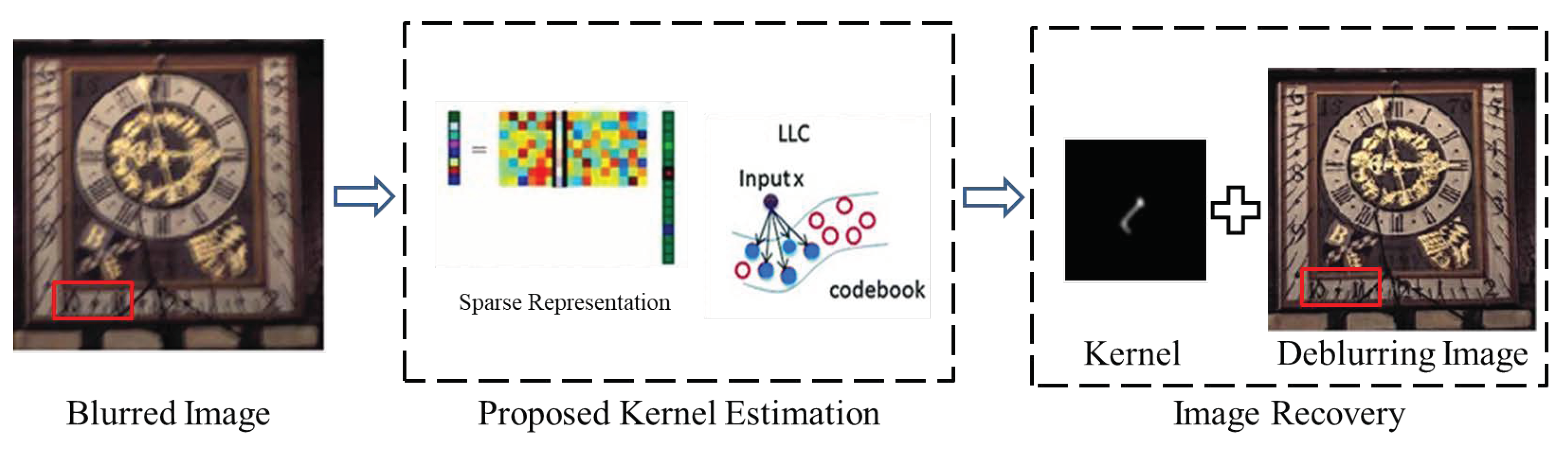
3. Method

In this section, the proposed method is presented to estimate blur kernel and an efficient minimization algorithm is developed to incorporate locality constraint. Some basic notations are presented in

Table 1. Notation and symbols.

Notation	Explanation
x	the latent sharp image
y	the input blurred image
k	the blur kernel
$\mathbf{N}$	the additive noise
*	the convolution operator
$D\in {\mathbb{R}}^{m\times n}$	the over-complete dictionary
$\alpha \in {\mathbb{R}}^{n\times n}$	the sparse coefficient matrix

.

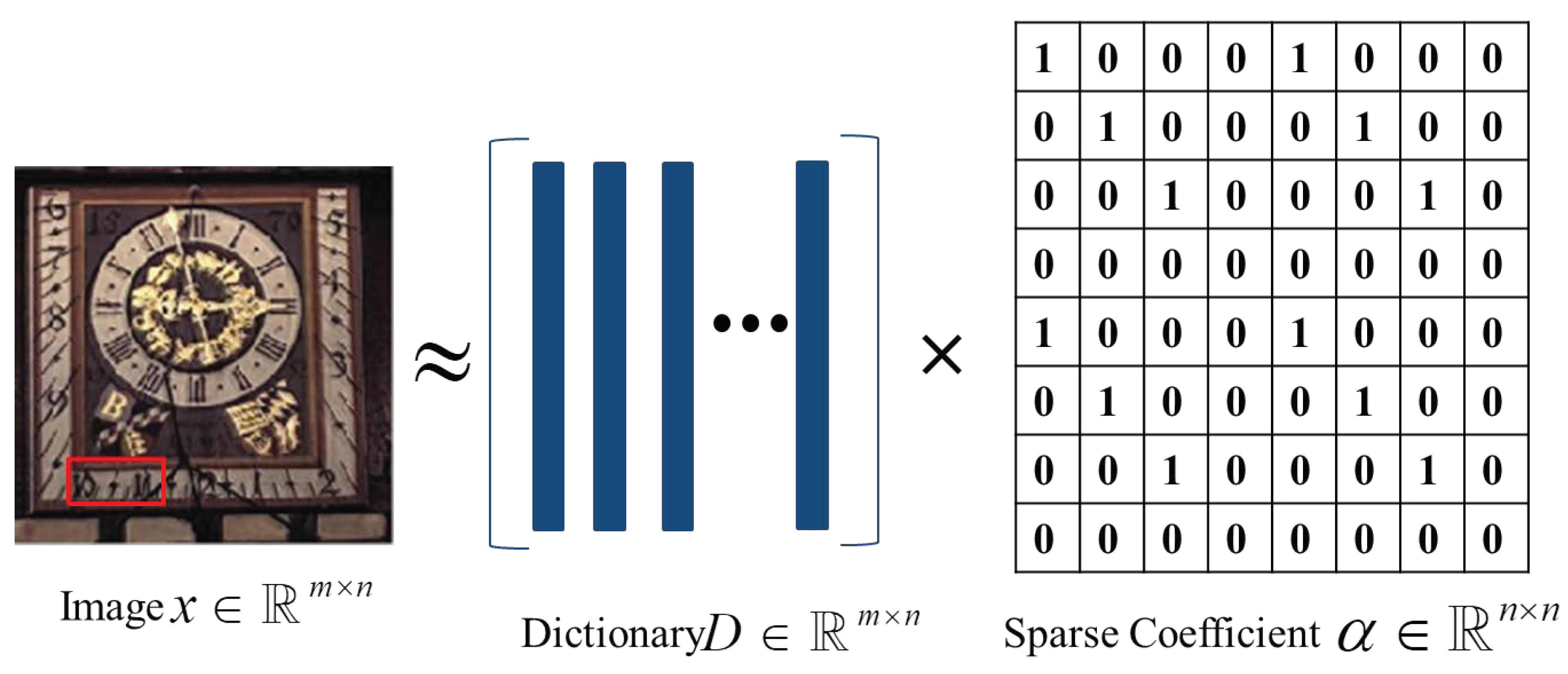
3.1. Sparse Representation

Sparse representation assumes that natural images can be sparsely represented under a basis or an overcomplete dictionary, which has been used in the field for several years. Let $x=[x_1,x_2,\dots ,x_n]\in {\mathbb{R}}^{m\times n}$ denote a clean image. Image x can be represented as

$$x=D\alpha ,$$

(2)

where $D=[D_1,D_2,\dots ,D_n]\in {\mathbb{R}}^{m\times n}$ is an over-complete dictionary with n atoms and $\alpha \in {\mathbb{R}}^{n\times n}$ is the sparse coefficient matrix. As shown in Figure 4, the sparse coefficient matrix $\alpha$ can be recovered by:

$$\begin{array}{c}\underset{\alpha }{min}{∥\alpha ∥}_0,\hfill \\ s.t.{∥x-D\alpha ∥}_2^2\le \epsilon ,\hfill \end{array}$$

(3)

where ${∥·∥}_0$ is the $l_0$ norm and $\epsilon \ge 0$ is the error tolerance. Generally, the optimization of $l_0$ norm problem is NP-hard. When $\alpha$ is sparse enough, Equation (3) can be solved through Lagrange multiplier, namely the following $l_1$ problem:

$$\widehat{\alpha }=\underset{\alpha }{argmin}||x-{D\alpha ||}_2^2+\lambda ||\alpha |{|}_1.$$

(4)

3.2. Structure Sparse Prior

A classic method for the blind deconvolution problem of Equation (1) is to solve the following objective function:

$$\{\widehat{x},\widehat{k}\}=\underset{x,k}{argmin}||y-{k\ast x||}_2^2+\eta \rho (x)+\gamma g(k),$$

(5)

where $\rho (x),g(k)$ is the regularization term on $x,k$, respectively, typically an $l_2$ norm penalty. With the sparsity prior as regularization, we can derive the following formulation:

$$\{\widehat{x},\widehat{k},\widehat{\alpha }\}=\underset{x,k,\alpha }{argmin}\left\{\begin{array}{c}||y-{k\ast x||}_2^2+\eta ||x-{D\alpha ||}_2^2\hfill \\ +\gamma g(k)+\beta \varphi (\alpha ),\hfill \end{array}\right\}$$

(6)

where $\varphi (\alpha )$ is the regularization term on $\alpha$, typically an $l_1$ norm penalty, and $\eta$, $\gamma$, and $\beta$ are the weight coefficients of different terms, respectively.

Considering the sparsity regularization and Locality-constrained Linear Coding (LLC) constraint, the proposed method exploits the structure relationships among pixels. LLC is a new coding scheme that considers the correlation between codes and ensures similar descriptors have similar codes, keeping the inherent nature of the image [25]. LLC uses the following criteria:

$$\underset{\alpha }{min}\sum _{i=1}^N||x_i-D{\alpha }_i|{|}^2+\lambda ||d_i\odot {\alpha }_i|{|}^2,$$

(7)

$$s.t.1^T{\alpha }_i=1,\forall i$$

where $D=[D_1,D_2,\dots ,D_n]$ and ⊙ denotes the element-wise multiplication. $d_i=exp(dist(x_i,D)/\sigma )$ and $dist(x_i,D_j)$ refers to the Euclidean distance between $x_i$ and $D_j$,

By introducing the sparsity regularization and the locality constraint, the objective function can be obtained as follows:

$$\underset{x,k,\alpha }{min}{||y-k\ast x||}_2^2+\eta ||x-{D\alpha ||}_2^2+{\lambda }_1||k|{|}_1+{\lambda }_2||d\odot {\alpha ||}_2^2,$$

(8)

where $d=[d_1,d_2,\dots ,d_n]$, $D=[D_1,D_2,\dots ,D_n]$, and ⊙ denotes the element-wise multiplication. $d_i=exp(dist(x_i,D)/\sigma )$, $dist(x_i,D)={[dist(x_i,D_1),dist(x_i,D_2),\dots ,dist(x_i,D_n)]}^T$, and $dist(x_i,D_j)$ refers to the Euclidean distance between $x_i$ and $D_j$.

We explain each term of the proposed objective function in Equation (8) in detail as follows.

• The first term in the objective function is a conventional constraint, which measures the likelihood between the recovered image and the blurred image.
• The second term means the recovered image is sparse representation.
• The third term represents the $l_1$-norm regularization on k to enforce sparsity.
• The last term, $||d\odot {\alpha ||}_2^2$, is the locality constraint, which ensures each descriptor is represented by multiple bases and regularizes the x and $\alpha$ at the same time.

The main purpose of the objective function in Equation (8) is to estimate the blur kernel. After the blur kernel is estimated, the final image can be recovered by a non-blind deconvolution algorithm (see next section for details). The proposed method combines LLC in the sparse regularization framework to keep the structure relationships among neighbor pixels in the blurred image during the blind deconvolution process. By taking the inherent attribute of the sharp image into consideration, the proposed method can get a more accurate kernel estimation.

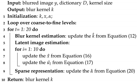
3.3. Optimization Procedure

The optimization problem in the proposed objective function in Equation (8) involves multiple variables, which is non-convex and hard to minimize directly. Fortunately, it is convex with respect to any one of the variables while fixing the other variables. Hence, we adopt the alternating minimization strategy by an iterative framework. The proposed objective function involves multiple variables, namely $x,k$, and $\alpha$, thus is hard to solve directly. An alternating minimization scheme is adopted, which reduces the original problem into three simpler sub-problems and alternately optimizes them. These three sub-problems of $x,k,\alpha$ are described as follows:

$$\widehat{k}=\underset{k}{argmin}||y-{k\ast x||}_2^2+{\lambda }_1||k|{|}_1,$$

(9)

$$\widehat{\alpha }=\underset{\alpha }{argmin}||x-{D\alpha ||}_2^2+{\lambda }_2||d\odot {\alpha ||}_2^2,$$

(10)

$$\widehat{x}=\underset{x}{argmin}||y-{k\ast x||}_2^2+\eta ||x-{D\alpha ||}_2^2+{\lambda }_2||d\odot {\alpha ||}_2^2.$$

(11)

Following this scheme, the sub-problems for optimizing each variable are addressed in an alternating fashion. In this case, the optimization problem can be solved by the following steps:

3.3.1. k Update

The k sub-problem is given by:

$$\widehat{k}=\underset{k}{argmin}||y-{k\ast x||}_2^2+{\lambda }_1||k|{|}_1,$$

(12)

$$s.t.\sum _i{k}_i=1,k\ge 0.$$

We can use the unconstrained iterative re-weighted least squares (IRLS) algorithm [8] to solve the problem. Similar to other deconvolution methods, we perform multiscale estimation of the kernel using a coarse-to-fine pyramid of image resolutions. To increase the robustness to noise, we set threshold to ensure small elements of the kernel are zero after recovering the kernel at the finest level.

3.3.2. x Update

The x sub-problem is given by:

$$\widehat{x}=\underset{x}{argmin}||y-{k\ast x||}_2^2+\eta ||x-{D\alpha ||}_2^2+{\lambda }_2||d\odot {\alpha ||}_2^2.$$

(13)

The third term, $||d\odot {\alpha ||}_2^2$, is a regularization on x, where $d=[d_1,d_2,\dots ,d_n]$, and $d_i$ is connected with $x_i$ and D. The element-wise multiplication of d and $\alpha$ makes it too difficult to solve x from the equation. Therefore, to make the problem easier to solve, an approximation can be applied to this sub-problem. We adopt the same regularization on x as Levin et al. [15], and the new object function becomes

$$\underset{x}{min}{∥y-k\ast x∥}_2^2+\eta {∥x-D\alpha ∥}_2^2+{\lambda }_2\sum _{l=1}^2{\left|e_l\ast x\right|}^s,$$

(14)

where $|e_l{\ast x|}^s$ takes the place of the third regularization term $||d\odot {\alpha ||}_2^2$ to get the problem solved more quickly. $e_l$ means a certain kind of derivative filter and typically $0.5\le s\le 0.8$. A new auxiliary variables $u_l(l\in 1,2)$ and the corresponding penalty term ${\sum }_{l=1}^2||u_l-e_l\ast x{||}_2^2$ are introduced in the function:

$$\underset{x,u_l}{min}||y-{k\ast x||}_2^2+\eta ||x-{D\alpha ||}_2^2+{\lambda }_2\sum _{l=1}^2|u_l{|}^s+\beta \sum _{l=1}^2{|u_l-e_l\ast x|}_2^2.$$

(15)

Similarly, the optimization problem can be divided into two sub-problems:

$$\widehat{x}=\underset{x}{argmin}||y-{k\ast x||}_2^2+\eta ||x-{D\alpha ||}_2^2+\beta \sum _{l=1}^2||u_l-e_l\ast x{||}_2^2,$$

(16)

$$\widehat{u_l}=\underset{u_l}{argmin}|u_l{|}^s+\beta ||u_l-e_l\ast x{||}_2^2.$$

(17)

The x sub-problem can be solved by FFT:

$$\widehat{x}=F^{-1}(\frac{\overline{F(k)}\odot F(y)+\eta F(D\alpha )+\beta {\sum }_{l=1}^2\overline{F(e_l)}\odot F(u_l)}{\overline{F(k)}\odot F(k)+\eta I+\beta {\sum }_{l=1}^2\overline{F(e_l)}\odot F(e_l)}),$$

(18)

where $F(·)$ represents Fast Fourier Transform (FFT), $F^{-1}(·)$ means inverse FFT, $\overline{F(·)}$ is the complex conjugate of $F(·)$, and ⊙ denotes element-wise multiplication.

As to $\widehat{u_l}$, we set $s=0.8,e_1=[1,-1]$, and $e_2={[1,-1]}^T$. Equation (17) can be solved efficiently through the algorithm proposed by Krishnan and Fergus [26].

3.3.3. $\alpha$ Update

The $\alpha$ sub-problem is given by:

$$\widehat{\alpha }=\underset{\alpha }{argmin}||x-{D\alpha ||}_2^2+{\lambda }_2||d\odot {\alpha ||}_2^2.$$

(19)

Inspired by Wang et al. [25], the solution of the sub-problem is

$$\widehat{{\alpha }_i}=(C_i+\lambda diag(d))\setminus 1,$$

(20)

$${\alpha }_i=\widehat{{\alpha }_i}/1^T\widehat{{\alpha }_i},$$

where $C_i=(D-1x_i^T){(D-1x_i^T)}^T$ denotes the data covariance matrix.

Details about the procedure of blur kernel estimation can be found in Algorithm 1. To start, we initialize the sparse representation $\alpha$ as that recovered from y with respect to D, and the latent sharp image x as $D\alpha$. Then, we fix two variables, namely x and $\alpha$, and update k. Similarly, x and $\alpha$ can be updated, respectively. We repeat the operation until obtaining a stable result of k.

Algorithm 1: Blur kernel estimation by structure sparse prior.

3.4. Final Image Recovery

After blur kernel estimation, a non-blind deblurring method is adopted to recover the final sharp image:

$$\underset{x}{min}\lambda ||k\ast x-{y||}_2^2+||{\nabla }_{x}y|{|}_{\alpha }+||{\nabla }_{y}y|{|}_{\alpha },$$

(21)

where ${\nabla }_x=[1,-1],{\nabla }_y={[1,-1]}^T$, $\lambda =3000$, and $\alpha =0.8$. The optimization approach can be obtained from Krishnan and Fergus [26]. This non-blind deblurring method is easy to solve and works very quickly.

4. Experiments and Results

In this part, details about experiments are described. In Section 4.1, the competitors and the metrics are introduced. In Section 4.2, the choices of parameters are presented. In Section 4.3, the results of the competitors and ours are compared.

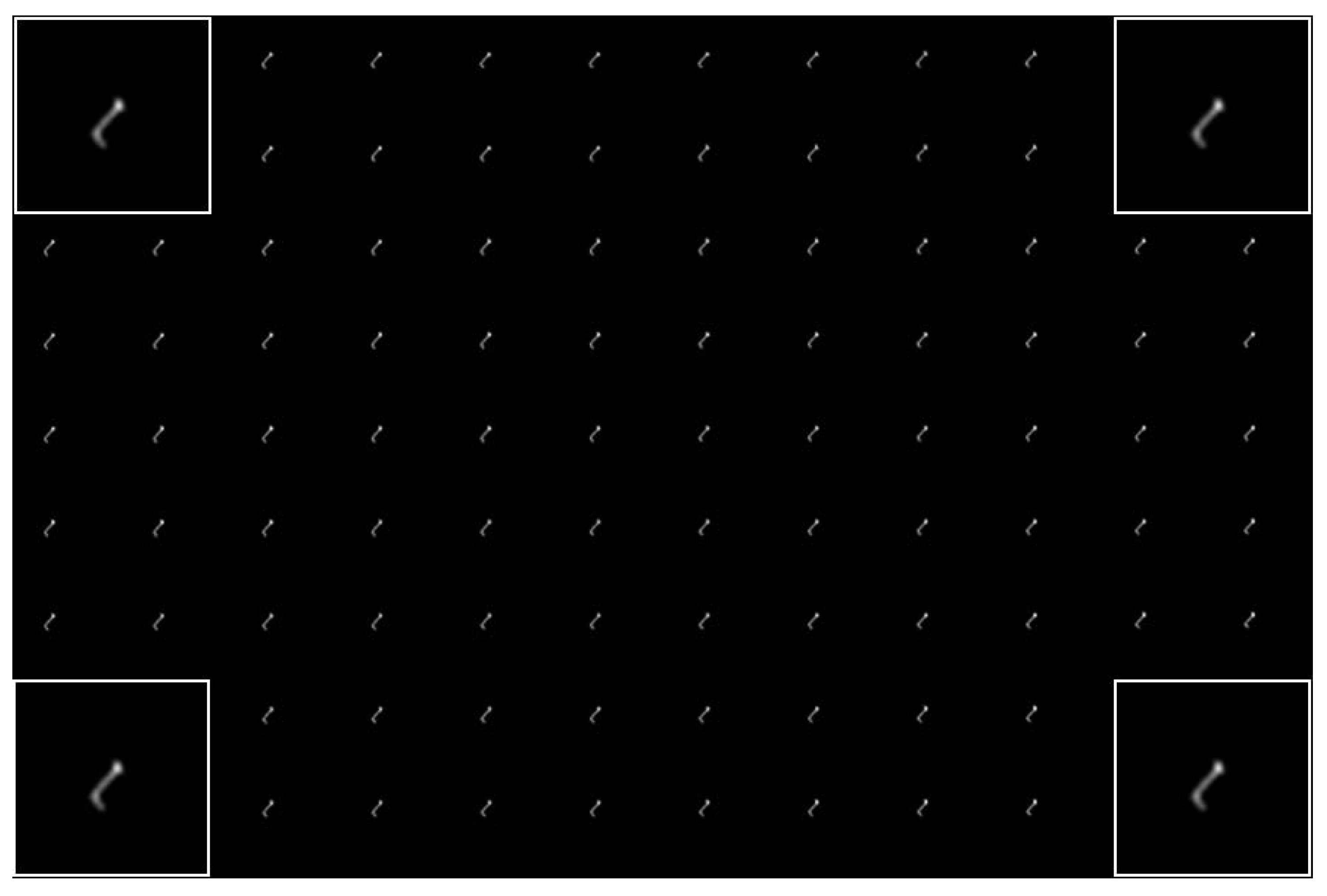
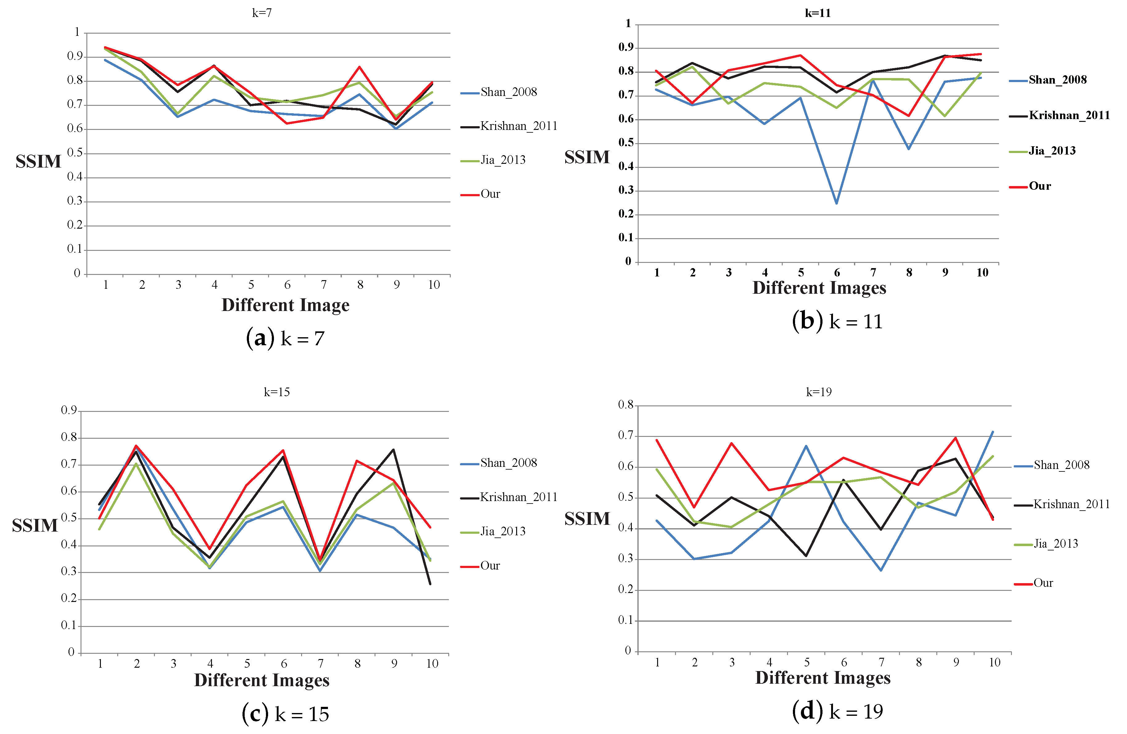
4.1. The Competitors and Experimental Images

To evaluate the proposed method, three different methods [8,27,28] were used as the competitors.

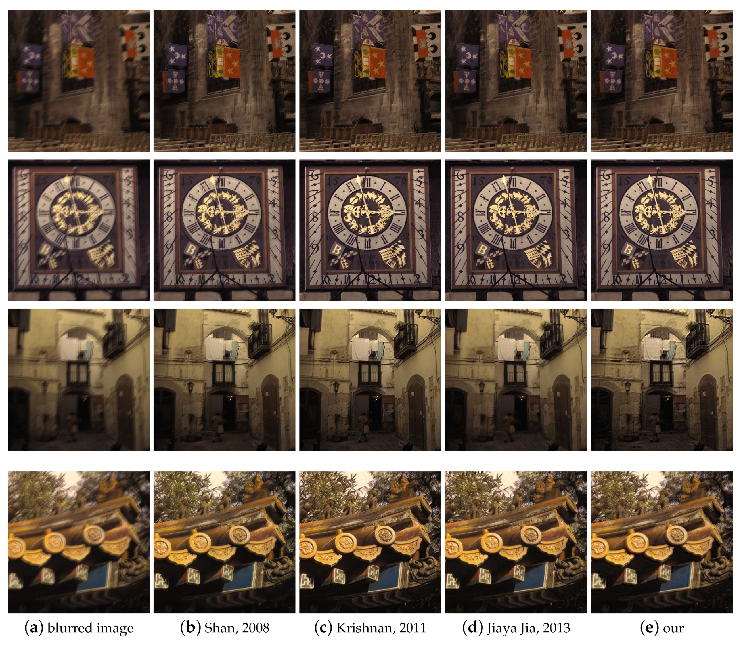
• Shan_2008: The first method is from Q. Shan et al. [27]. The method recovers the clear image in a unified probabilistic model, including blur kernel estimation and image restoration.
• Krishnan_2011: The second method is from D. Krishnan et al. [8]. The method introduces a new type of regularization term, namely $l_1/l_2$ norm, which gives lowest cost for the true sharp image.
• Jia_2013: The final method is from L. Xu et al. [28]. The method provides a unified framework for removing the blur kernel. A generalized and mathematically sound $l_0$ sparse expression is proposed.

In fact, two kinds of experiments from different perspectives were conducted. First, the experiment on the recovery performance of the proposed method was conducted on the benchmark from Köhler et al. [29]. Then, the experiment on robustness was conducted on Berkeley Segmentation Database (http://www.eecs.berkeley.edu/Research/Projects/CS/vision/grouping/segbench) [30]. We chose 40 images from this database and randomly divided them into four groups (10 images in each group). Then, we generated blurred images with different blur kernels, where the kernel size was 7–19 pixels (kernel size = 7, 11, 15, 19). To evaluate the performances of comparison, two quantitative metrics were considered: Structure SIMilarity (SSIM) and Peak Signal to Noise Ratio (PSNR). These metrics evaluate the performances by comparing the similarity between the original image and the deblured image.

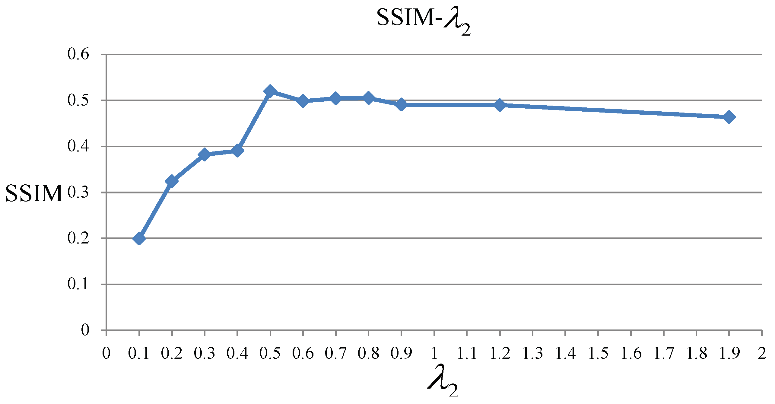
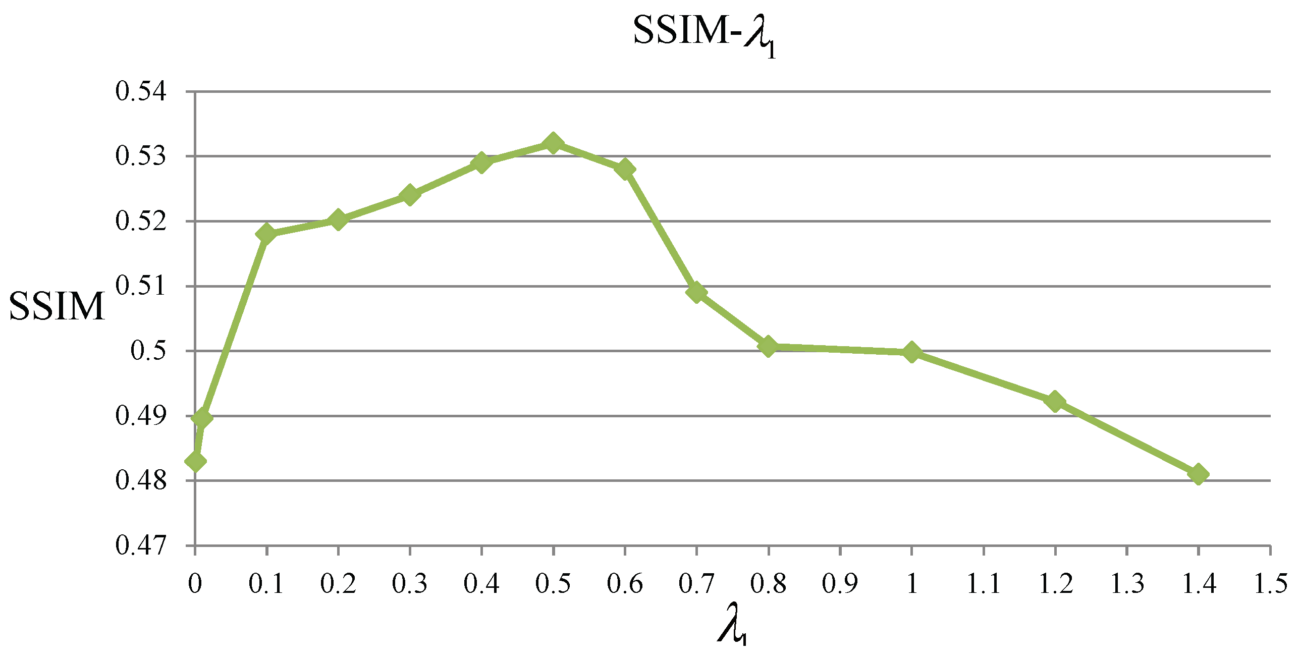
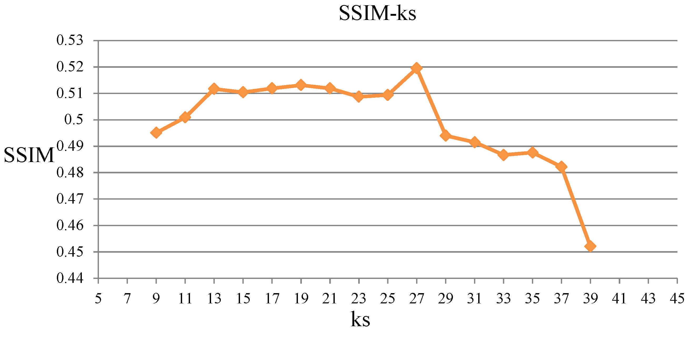
4.2. Evaluation of The Parameters

In the proposed method, four parameters can be adjusted to improve the deblurring performance: $\eta ,{\lambda }_1$, ${\lambda }_2$ and $ks$. Among them, ${\lambda }_1$ is the weight coefficient in Equation (10); $\eta$ and ${\lambda }_2$ are the weight coefficients in Equation (12); and $ks$ represents the size of kernel k. The size of kernel k was initialized as $3\times 3$ and it grew with the ratio of $\sqrt{2}$ between different levels. The number of levels was decided by the final size of kernel k.

We set $\eta =0.001$, while the size of kernel, ${\lambda }_1$, and ${\lambda }_2$ were flexible to ensure the best recovery effect for different input images. The parameters were initialized as follows: $ks=19,{\lambda }_1=0.1$, and ${\lambda }_2=0.5$.

First, we fixed ${\lambda }_1$ and ${\lambda }_2$, and chose the best $ks$ for kernel estimation. If the kernel size we set were too small or too large, it would not be good for accurately estimating the kernel. Experimental results can be found in Figure 5, from which we can get that the best size of kernel is 27. Then we fixed $ks$ and ${\lambda }_1$ and chose the best value for ${\lambda }_2$. If the ${\lambda }_2$ we set were too small, it would not have the effect of stabilizing the solution and the regularization term on x would have little influence in the process. However, if ${\lambda }_2$ were too large, x would be over constrained. Experimental result can be found in Figure 6, from which we can get that the best value for ${\lambda }_2$ is 0.5. Finally we fixed $ks$ and ${\lambda }_2$ and chose the best value for ${\lambda }_1$. Similarly, ${\lambda }_1$ cannot be too large as k would be over constrained. However, if ${\lambda }_1$ were too small, the regularization on k would not have the function of enforcing sparsity. Experimental result can be found in Figure 7, from which we can get that the best value for ${\lambda }_1$ is 0.5.

4.3. Result

In this section, several experimental evaluations are presented. The PSNR and SSIM values with various deblurring methods are shown in

Table 2. Comparison on four images from a real-world benchmark dataset. SSIM values of the debluring images by different methods.

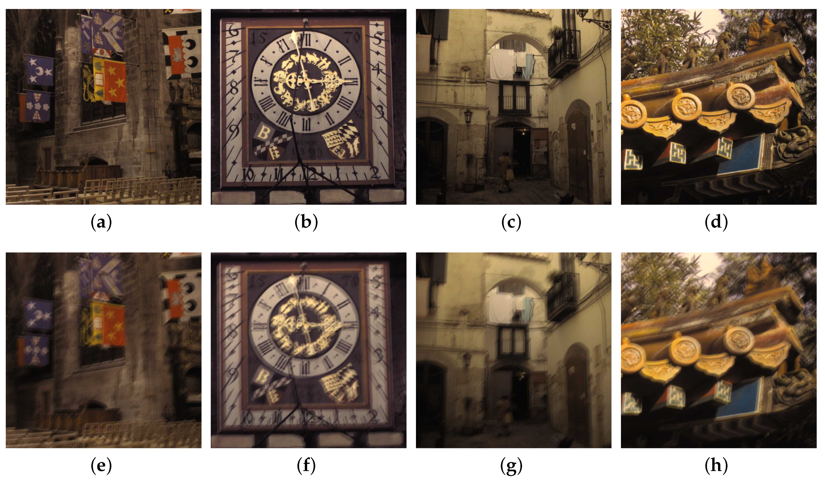
Image	Image Size	Shan [27]	Krishnan [8]	Jia [28]	Our
Image1 (church)	800 × 800	0.5884	0.6145	0.6128	0.6180
Image2 (clock)	800 × 800	0.334	0.2874	0.3872	0.4847
Image3 (backyard)	800 × 800	0.6395	0.6245	0.6463	0.6851
Image4 (roof)	800 × 800	0.4899	0.4748	0.4819	0.5200

and

Table 3. Comparison on four images from a real-world benchmark dataset. PSNR values of the debluring images by different methods.

Image	Image Size	Shan [27]	Krishnan [8]	Jia [28]	Our
Image1 (church)	800 × 800	23.05	22.951	23.031	23.3618
Image2 (clock)	800 × 800	26.002	28.448	28.448	28.521
Image3 (backyard)	800 × 800	22.1814	21.6318	22.197	23.3827
Image4 (roof)	800 × 800	18.1483	17.1282	17.6505	18.9445

, respectively. It can be seen that our proposed method can achieve higher SSIM and PSNR than other methods. Besides, Figure 8 shows the corresponding visual illustration. It is observed that our proposed method obtains better performance compared with other methods. The reason is that the proposed method takes into account the structure relationship among neighbor pixels of the input image to help alleviate the ill-posed problem. Figure 9 shows the blur kernel estimation by different methods. The proposed method achieves better blur field than the competitors.

In experiments, the parameters should be adjusted for each test image. To verify the effectiveness of our proposed method, experiments with different the size of kernel were conducted. Figure 10 shows the SSIM values with different kernel sizes. The comparison results of different methods in regard to SSIM are shown. Figure 10 shows that our proposed method achieves the best SSIM performance most of the time under different kernel sizes. No parameters were changed except the size of the kernel. It can be seen that our proposed method has its advantage in different kernel sizes. The reason is that both the sparsity regularization and the locality constraint are incorporated to obtain less reconstruction error and preserve the structure information of the image.

5. Discussion

From the experiments, we can see that the proposed method achieves better performance than the competitors. The experimental results show that structure sparse prior can improve the performance of image deblurring. Both the sparsity regularization and the locality constraint are incorporated to exploit the structure relationships among pixels. We further observe that the proposed method obtains the best SSIM index for most cases, which indicates the effective of the proposed method.

6. Conclusions

In this paper, a novel blur kernel estimation method is proposed, which incorporates the sparsity prior and the locality constraint. To avoid the weakness of sparse representation, the proposed method utilizes the correlations between different image pixels. A structure sparse prior is proposed by introducing the locality constraint into sparse representation framework. By utilizing the locality constraint and the sparsity regularization, the proposed method can preserve the structure information of image. The structure sparse prior can preserve the inherent attribute of the sharp image. Extensive experiments showed that the proposed method outperforms other deblurring methods.

References

- Uzer, F. Camera Motion Blur and Its Effect on Feature Detectors. Master’s Thesis, Middle East Technical University, Ankara, Turkey, 2010. [Google Scholar]
- Zheng, X.; Yuan, Y.; Lu, X. Hyperspectral Image Denoising by Fusing the Selected Related Bands. IEEE Trans. Geosci. Remote Sens. 2019, 57, 2596–2609. [Google Scholar] [CrossRef]
- Donatelli, M.; Estatico, C.; Martinelli, A.; SerraCapizzano, S. Improved image deblurring with antireflective boundary conditions and reblurring. Inverse Probl. 2006, 22, 2035–2053. [Google Scholar] [CrossRef]
- Levin, A.; Fergus, R.; Durand, F.; Freeman, W.T. Image and depth from a conventional camera with a coded aperture. ACM Trans. Graph. 2007, 26, 70. [Google Scholar] [CrossRef]
- Yuan, L.; Sun, J.; Quan, L.; Shum, H.Y. Progressive inter-scale and intra-scale non-blind image deconvolution. ACM Trans. Graph. 2008, 27, 74. [Google Scholar] [CrossRef]
- Gupta, A.; Joshi, N.; Zitnick, L.; Cohen, M.; Curless, B. Single image deblurring using motion density functions. In European Conference on Computer Vision; Springer: Berlin/Heidelberg, Germany, 2010; pp. 171–184. [Google Scholar]
- Bar, L.; Sapiro, G. Generalized Newton methods for energy formulations in image procesing. In Proceedings of the IEEE International Conference on Image Processing, San Diego, CA, USA, 12–15 October 2008; pp. 809–812. [Google Scholar]
- Krishnan, D.; Tay, T.; Fergus, R. Blind deconvolution using a normalized sparsity measure. In Proceedings of the IEEE Conference on Computer Vision and Pattern Recognition, Providence, RI, USA, 20–25 June 2011; pp. 233–240. [Google Scholar]
- Levin, A.; Weiss, Y.; Durand, F.; Freeman, W.T. Understanding and evaluating blind deconvolution algorithms. In Proceedings of the IEEE Conference on Computer Vision and Pattern Recognition, Miami, FL, USA, 20–25 June 2009; pp. 1964–1971. [Google Scholar]
- Chen, Y.; Ding, J.; Lai, W.; Chen, Y.; Chang, C.W.; Chang, C.C. High Quality Image Deblurring Scheme Using the Pyramid Hyper-Laplacian L2 Norm Priors Algorithm. In Pacific-Rim Conference on Multimedia; Springer: Cham, Switzerland, 2013; pp. 134–145. [Google Scholar]
- Almeida, M.; Almeida, L. Blind and semi-blind deblurring of natural images. IEEE Trans. Image Process. 2010, 19, 36–52. [Google Scholar] [CrossRef] [PubMed]
- Dong, W.; Shi, G.; Li, X. Image Deblurring with Low-rank Approximation Structured Sparse Representation. In Proceedings of the Signal & Information Processing Association Annual Summit and Conference, Hollywood, CA, USA, 3–6 December 2012; pp. 1–5. [Google Scholar]
- Wipf, D.P.; Zhang, H. Revisiting Bayesian Blind Deconvolution. J. Mach. Learn. Res. 2014, 15, 3595–3634. [Google Scholar]
- Babacan, S.; Molina, R.; Do, M.N.; Katsaggelos, A.K. Bayesian blind deconvolution with general sparse image priors. In Proceedings of the European Conference on Computer Vision, Florence, Italy, 7–13 October 2012; pp. 341–355. [Google Scholar]
- Levin, A.; Weiss, Y.; Durand, F.; Freeman, W. Efficient marginal likelihood optimization in blind deconvolution. In Proceedings of the IEEE Conference on Computer Vision and Pattern Recognition, Providence, RI, USA, 20–25 June 2011; pp. 2657–2664. [Google Scholar]
- Fergus, R.; Singh, B.; Hertzmann, A.; Roweis, S.T.; Freeman, W.T. Removing camera shake from a single photograph. ACM Trans. Graph. 2006, 25, 787–794. [Google Scholar] [CrossRef]
- Zhang, H.; Wipf, D.; Zhang, Y. Multi-Observation Blind Deconvolution with an Adaptive Sparse Prior. IEEE Trans. Pattern Anal. Mach. Intell. 2014, 36, 1628–1643. [Google Scholar] [CrossRef] [PubMed]
- Cho, T.; Joshi, N.; Zitnick, C.L.; Sing, K.; Szeliski, R.; Freeman, W.T. A content-aware image prior. In Proceedings of the IEEE Conference on Computer Vision and Pattern Recognition, San Francisco, CA, USA, 13–18 June 2010; pp. 169–176. [Google Scholar]
- Cai, J.; Hui, J.; Liu, C.; Shen, Z. Blind motion deblurring from a single image using sparse approximation. In Proceedings of the IEEE Confernece on Computer Vision and Pattern Recognition, Miami, FL, USA, 20–25 June 2009; pp. 104–111. [Google Scholar]
- Aharon, M.; Elad, M.; Bruckstein, A. K-svd: An algorithm for designing overcomplete dictionaries for sparse representation. IEEE Trans. Signal Process. 2006, 54, 4311–4322. [Google Scholar] [CrossRef]
- Zhang, H.; Yang, J.; Nasrabadi, N.M.; Huang, T.S. Close the loop: Joint blind image restoration and recognition with sparse representation prior. In Proceedings of the IEEE Confenece on Computer Vision and Pattern Recognition, Barcelona, Spain, 6–13 November 2011; pp. 770–777. [Google Scholar]
- Jia, C.; Brain, L. Patch-based image deconvolution via joint modeling of sparse priors. In Proceedings of the IEEE International Conference on Image Processing, Brussels, Belgium, 11–14 September 2011; pp. 681–684. [Google Scholar]
- Elad, M.; Figueiredo, M.; Ma, Y. On the role of sparse and redundant representations in image processing. Proc. IEEE 2010, 98, 972–982. [Google Scholar] [CrossRef]
- Cho, S.; Lee, S. Fast motion deblurring. ACM Trans. Graph. 2009, 28, 145. [Google Scholar] [CrossRef]
- Wang, J.; Yang, J.; Yu, K.; Lv, F.; Huang, T. Locality-constrained linear coding for image classification. In Proceedings of the IEEE Conference on Computer Vision and Pattern Recognition, San Francisco, CA, USA, 13–18 June 2010; pp. 3360–3367. [Google Scholar]
- Krishnan, D.; Fergus, R. Fast image deconvolution using hyper-Laplacian priors. In Proceedings of the Advances in Neural Information Processing Systems, Vancouver, BC, Canada, 7–10 December 2009; pp. 1033–1041. [Google Scholar]
- Shan, Q.; Jia, J.; Agarwala, A. High-Quality Motion Deblurring from a Single Image. ACM Trans. Graph. 2008, 27, 73. [Google Scholar] [CrossRef]
- Xu, L.; Zheng, S.; Jia, J. Unnatural L0 Sparse Representation for Natural Image Deblurring. In Proceedings of the IEEE International Conference on Image Processing, Portland, OR, USA, 23–28 June 2013; pp. 1107–1114. [Google Scholar]
- Köhler, R.; Hirsch, M.; Mohler, B.; Schölkopf, B.; Harmeling, S. Recording and playback of camera shake: Benchmarking blind deconvolution with a real-world database. In European Conference on Computer Vision; Springer: Berlin/Heidelberg, Germany, 2012; pp. 27–40. [Google Scholar]
- Martin, D.; Fowlkes, C.; Tal, D.; Malik, J. A Database of Human Segmented Natural Images and its Application to Evaluating Segmentation Algorithms and Measuring Ecological Statistics. In Proceedings of the 8th International Conference on Computer Vision, Vancouver, BC, Canada, 9–12 July 2001; pp. 416–423. [Google Scholar]