Heat Transfer Performance of Fruit Juice in a Heat Exchanger Tube Using Numerical Simulations


Abstract
1. Introduction
2. Numerical Simulations
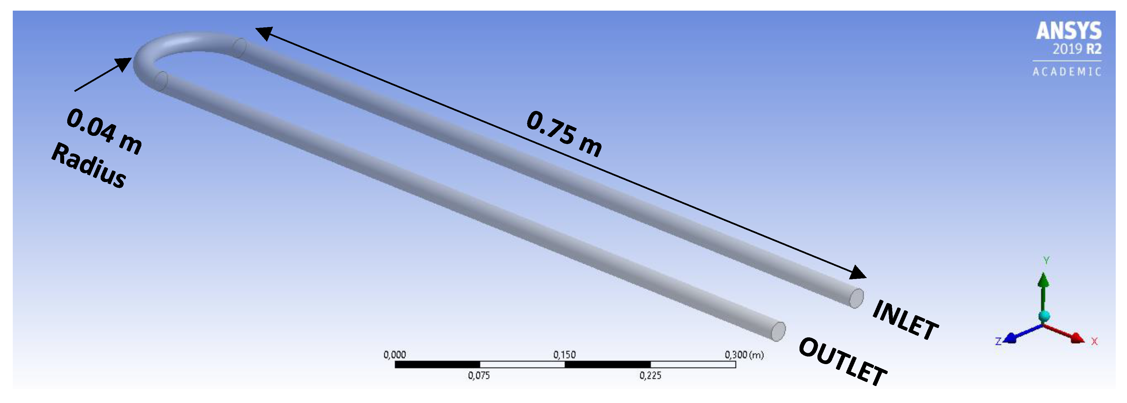
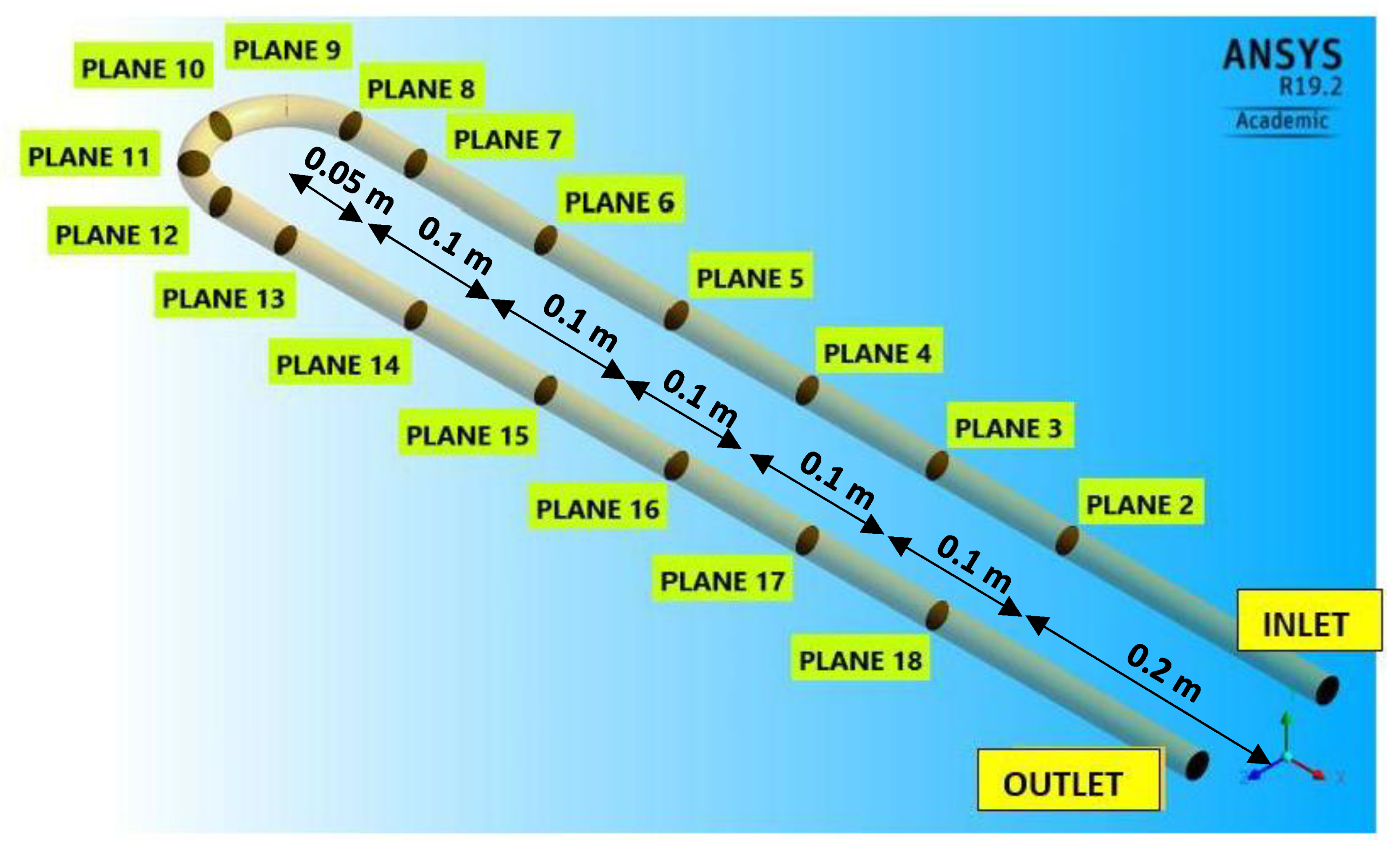
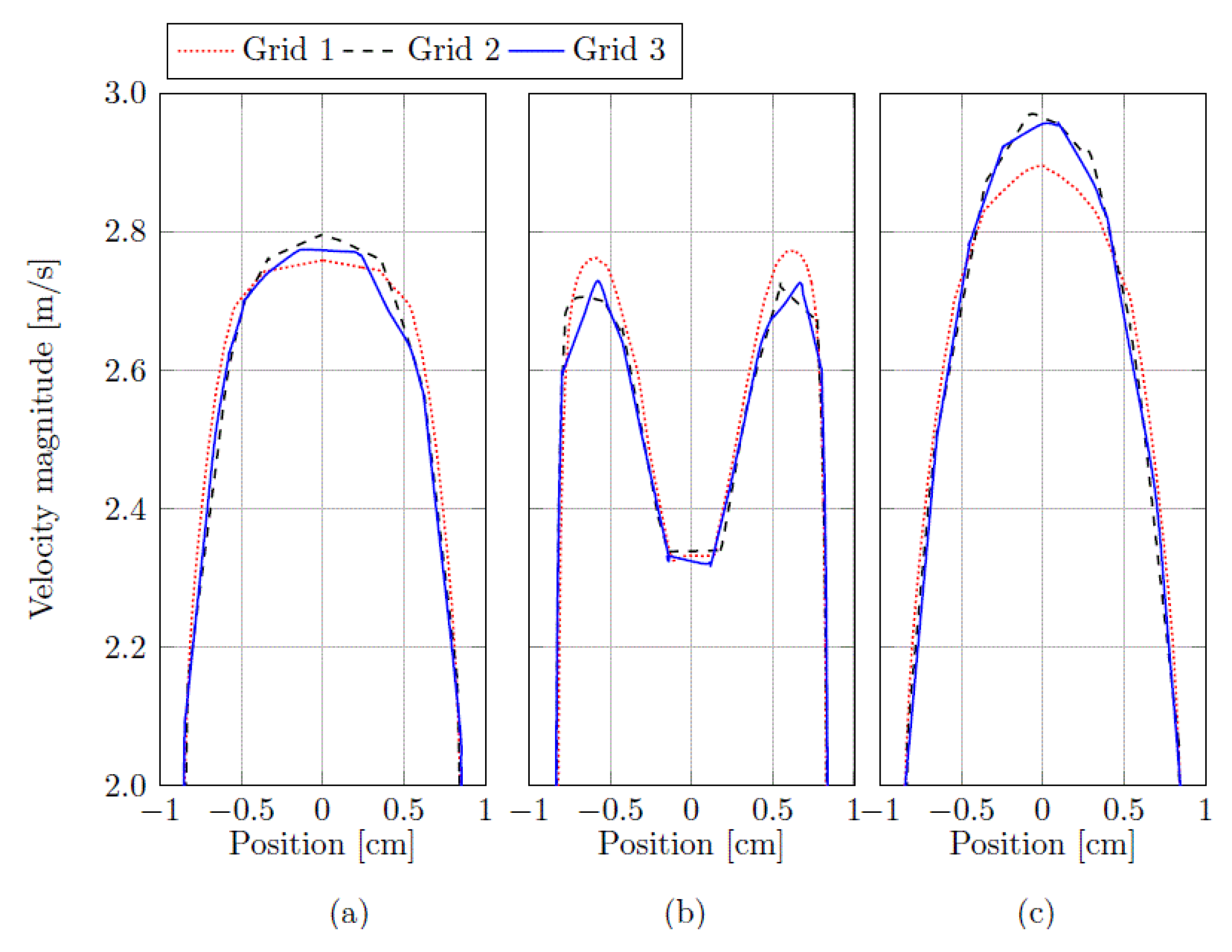
2.1. Case Study and Mesh Generation
2.2. Governing Equations
2.3. Boundary Conditions
2.4. Numerical Procedure
3. Results and Discussion
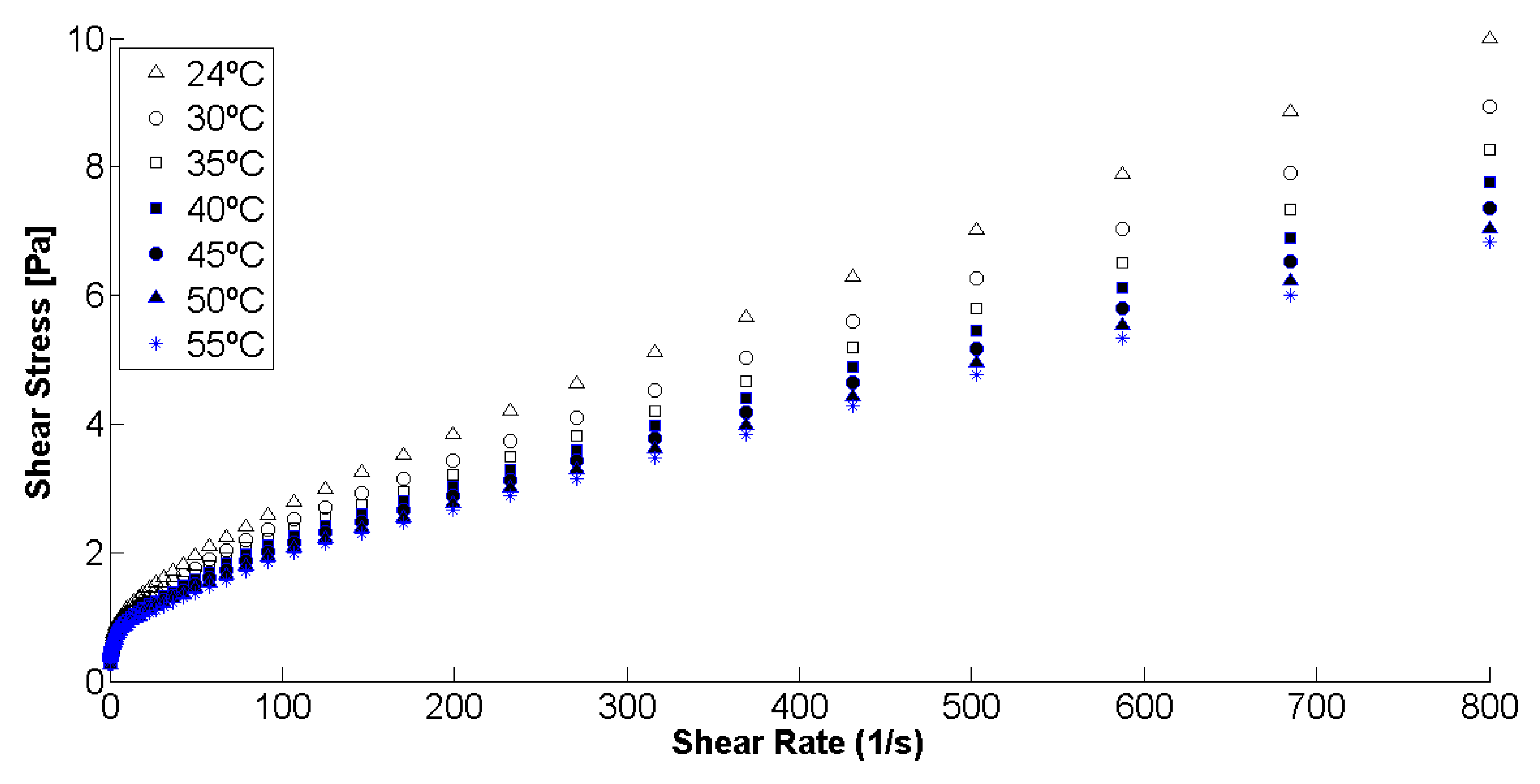
3.1. Rheological Measurements
3.2. Model Validation with Liquid Water
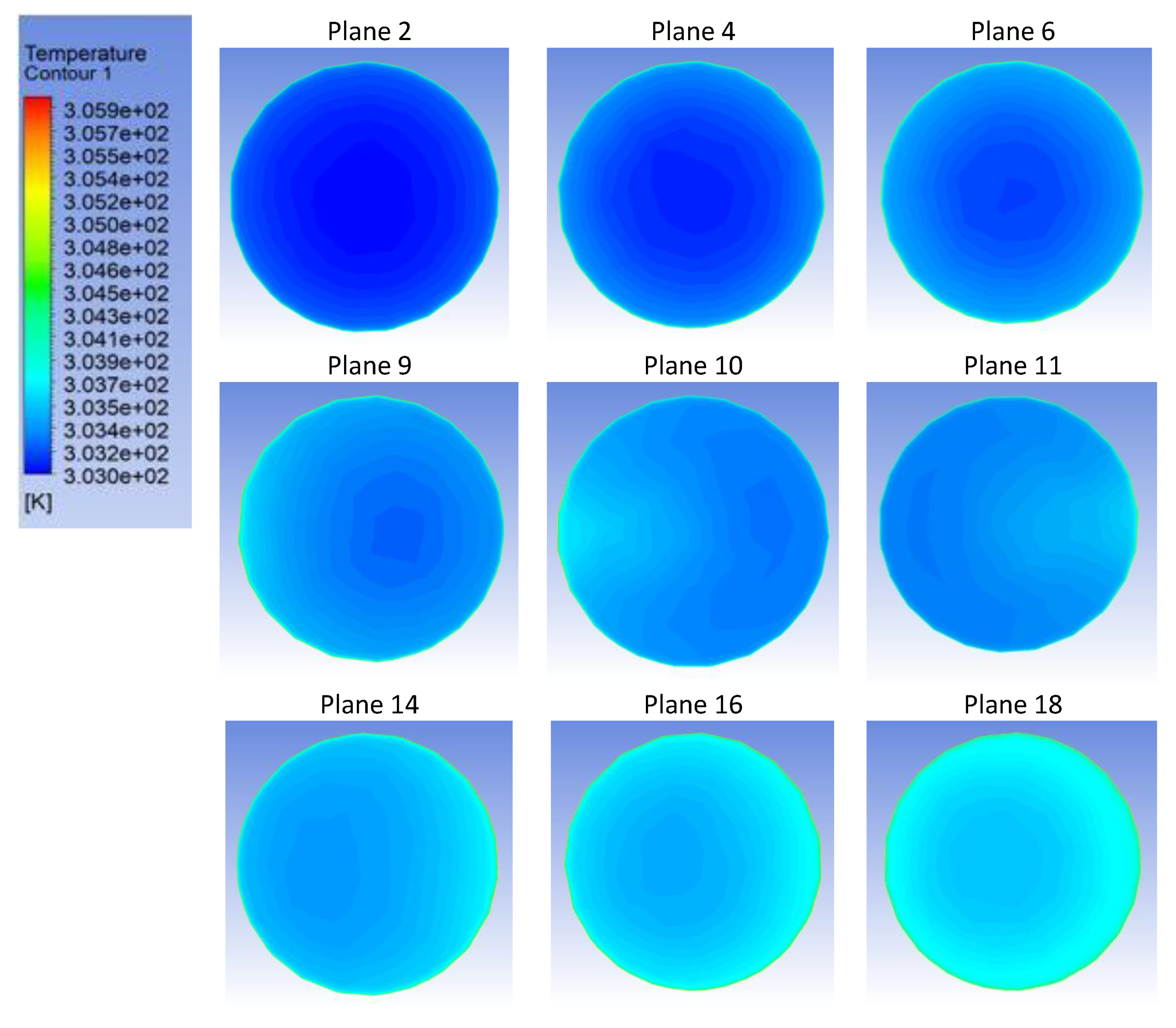
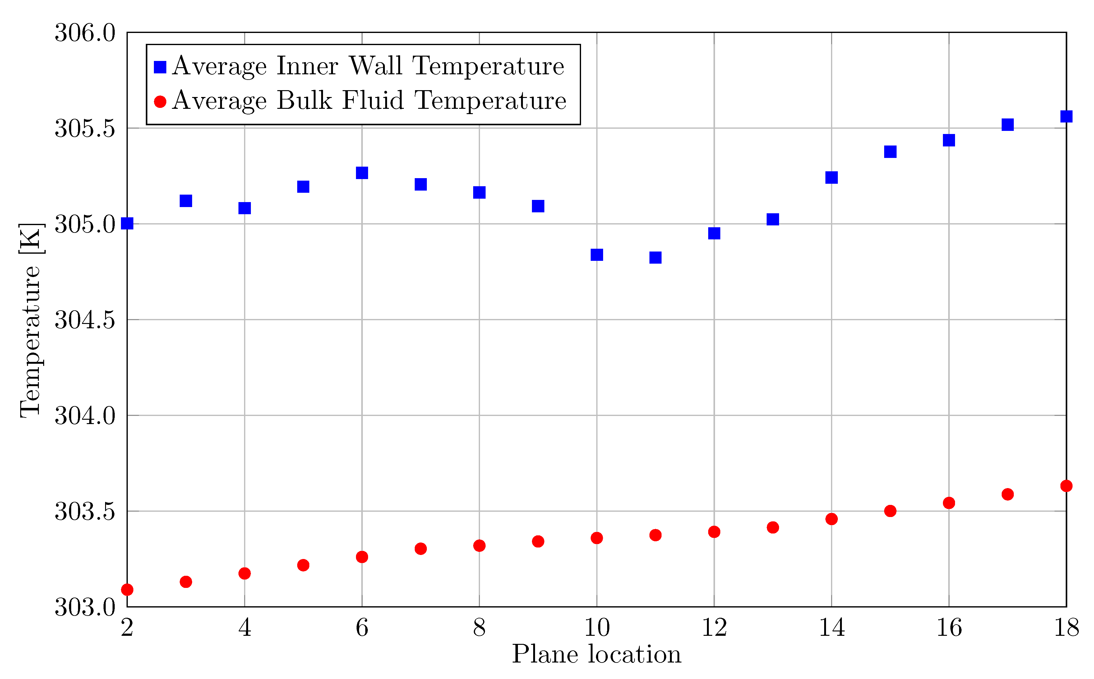
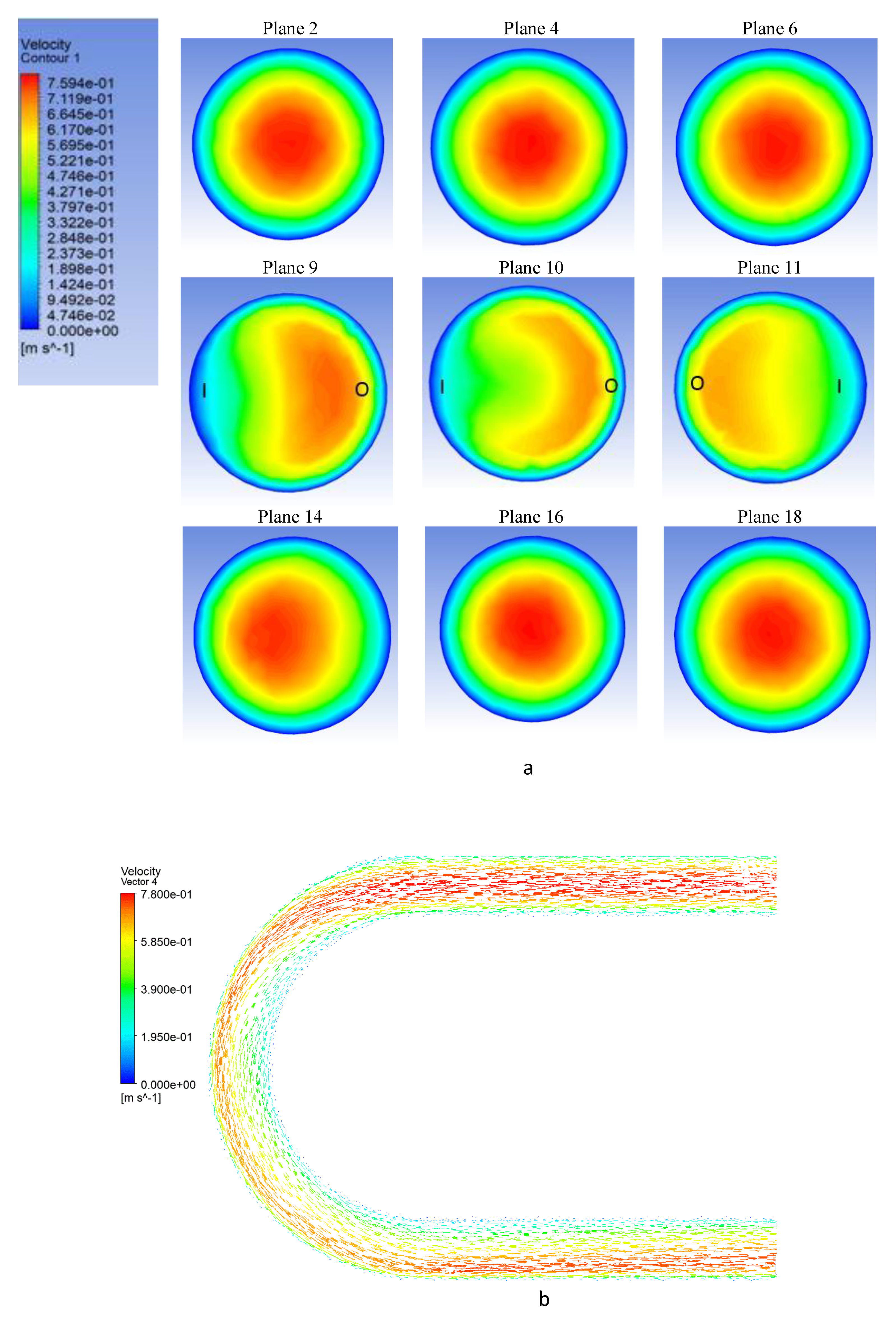
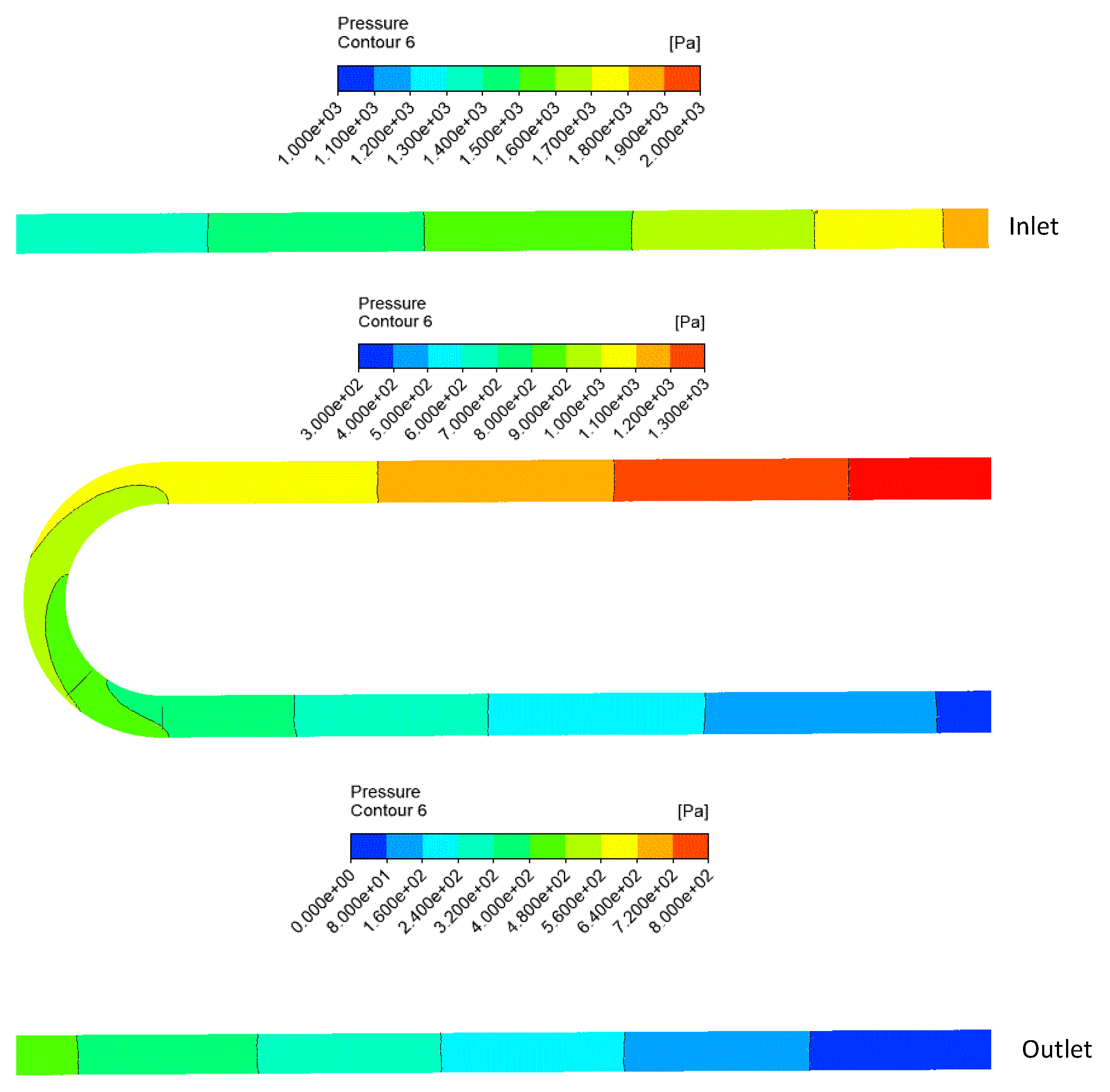
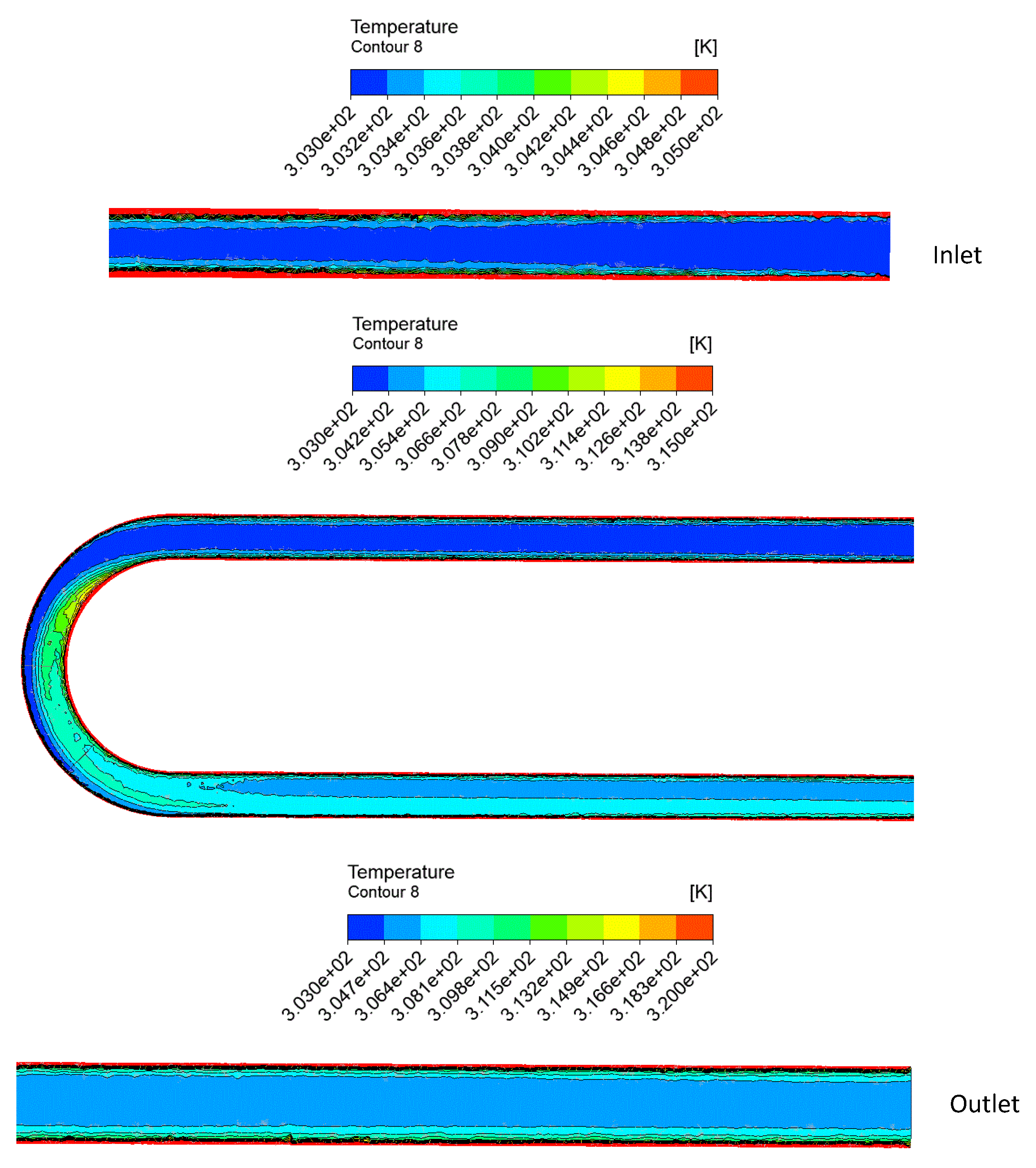
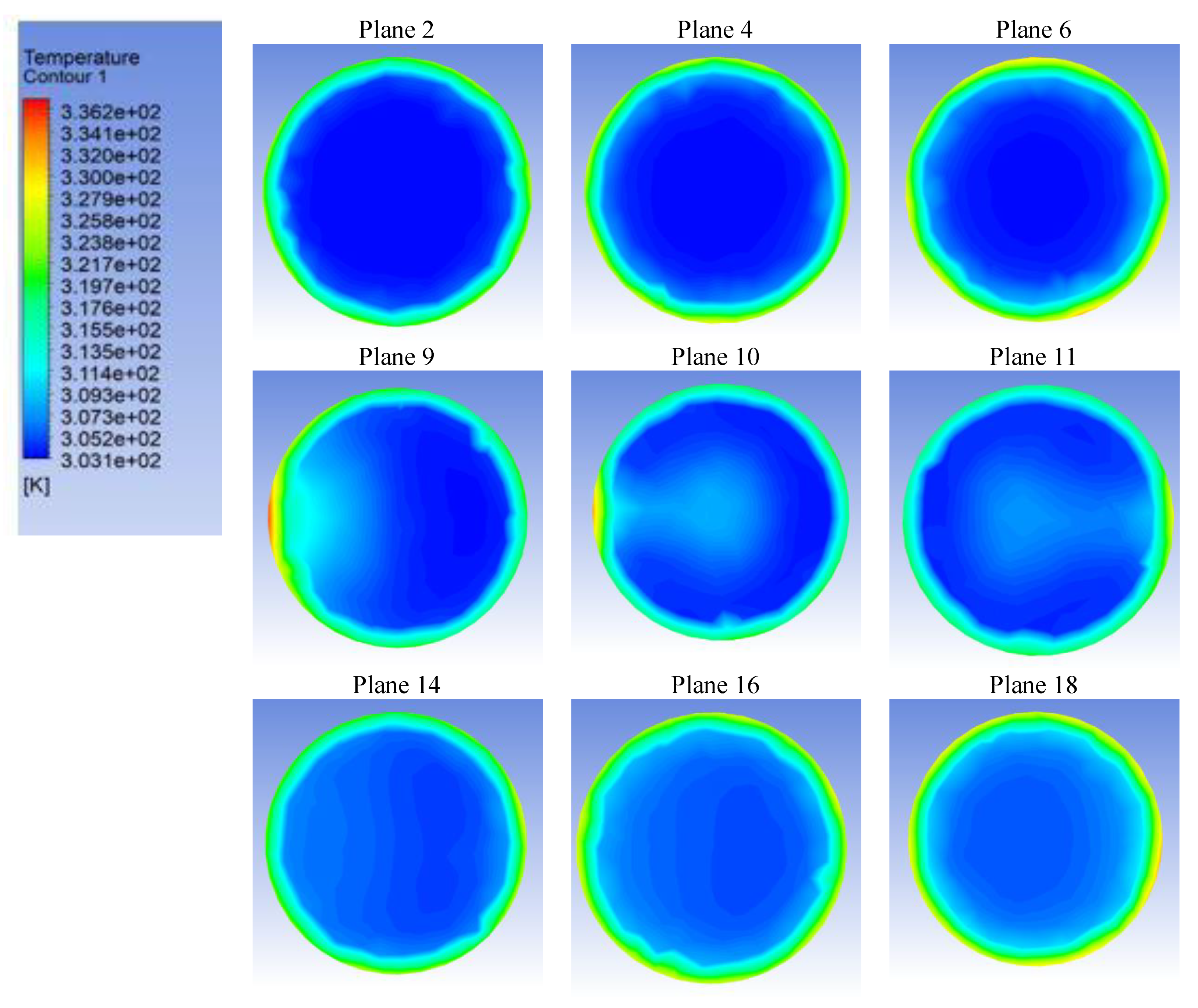
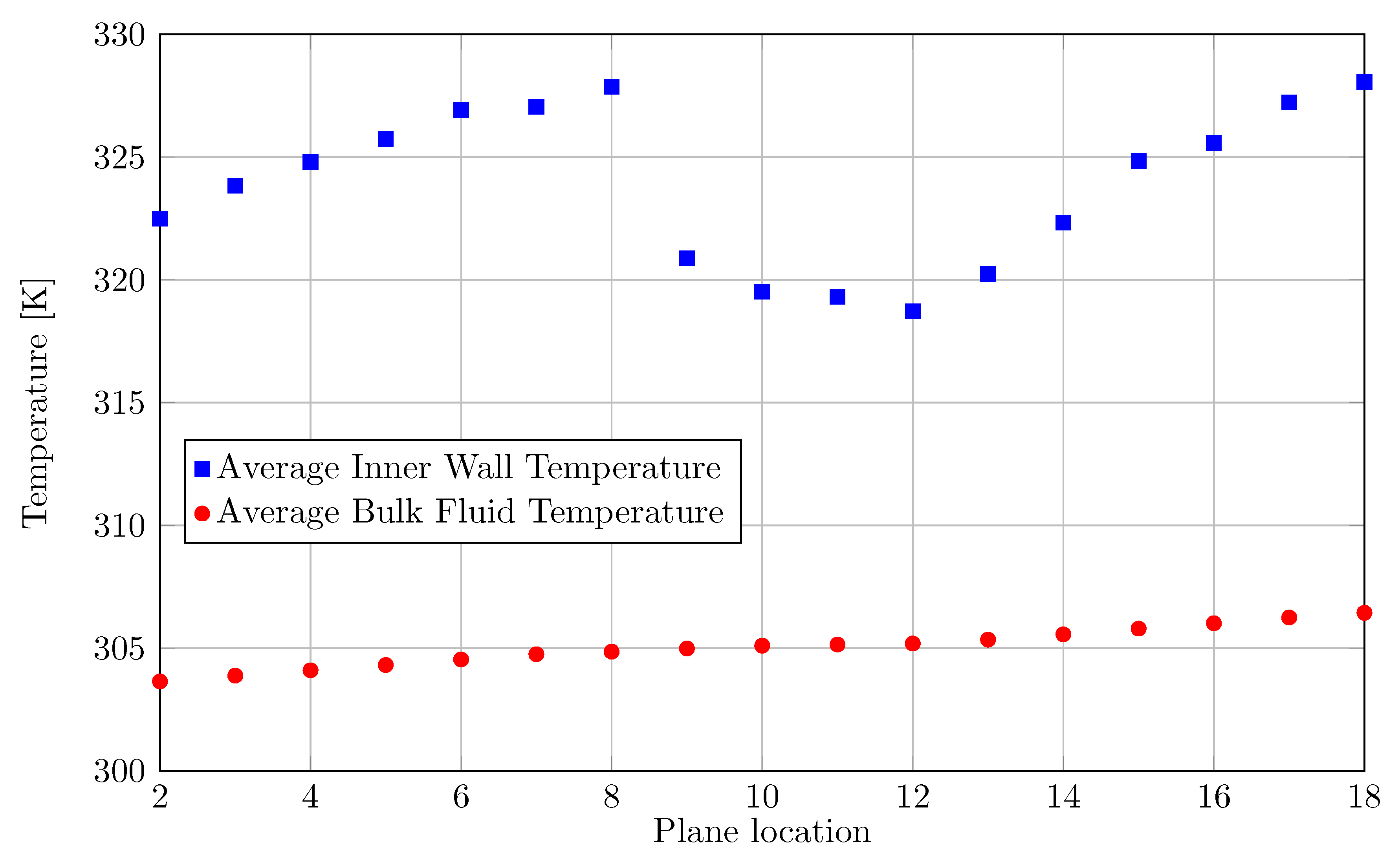
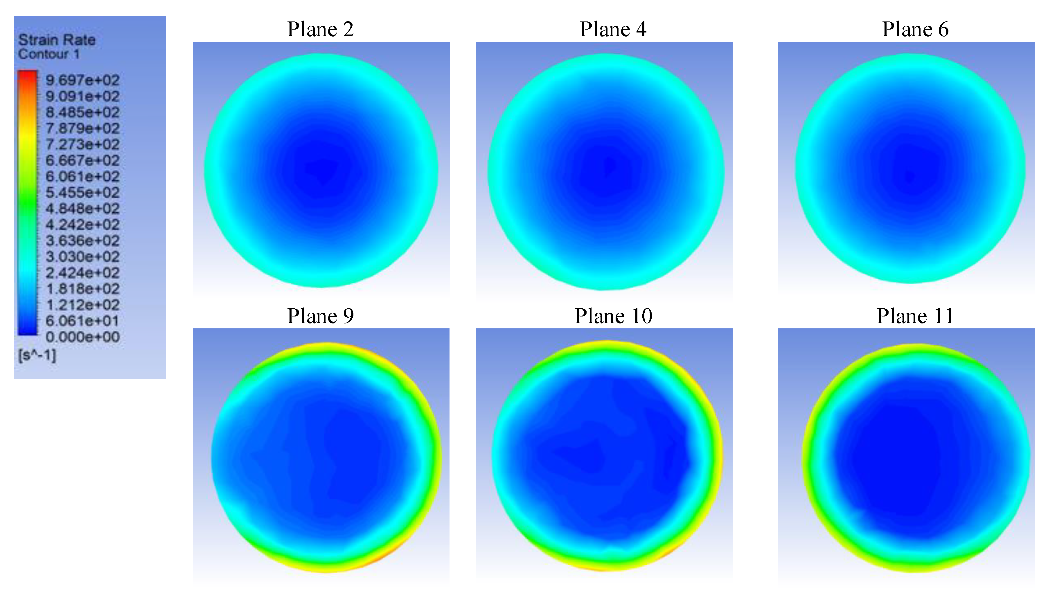
3.3. Simulation Results with a Non-Newtonian Fruit Juice in Laminar Regime
4. Conclusions
Author Contributions
Funding
Acknowledgments
Conflicts of Interest
Notation
| A | Constant (Pa·s) |
| a | Tube inside radius (mm) |
| , | turbulence model constants |
| Computational Fluid Dynamics | |
| Fanning friction factor | |
| Fanning friction factor for curved tube | |
| Fanning friction factor for straight tube | |
| Specific heat (J/(kg K)) | |
| D | Inner tube diameter (m) |
| De | Dean number |
| Hydraulic diameter (m) | |
| Activation energy () | |
| Generation of turbulent kinetic energy due to buoyancy | |
| Generation of turbulent kinetic energy due to the mean velocity gradients | |
| Graetz number | |
| Local heat transfer coefficient (W/(mK)) | |
| Heat Transfer Fluid | |
| I | Turbulent intensity (%) |
| K | Consistency index (Pa·s) |
| Constant (Pa·s) | |
| Loss coefficient in a bend | |
| L | Length (m) |
| Length of the straight tube (m) | |
| n | Flow behaviour index |
| Average Nusselt number | |
| Nusselt for curved coil | |
| Nusselt for straight tube in turbulent regime | |
| Nusselt for straight tube in laminar regime | |
| Local Nusselt number | |
| p | Pressure (Pa) |
| Pressure outlet (Pa) | |
| Prandtl number | |
| Turbulent Prandtl number | |
| Heat transfer flux (W/m) | |
| R | Radius of curvature (mm) |
| Reynolds number | |
| Generalised Reynolds number | |
| Universal gas constant () | |
| Deformation tensor | |
| Mean strain-rate of the flow | |
| User-defined source term | |
| User-defined source term | |
| T | Temperature (K) |
| Average temperature of the fluid at position x (K) | |
| Average inner wall temperature at position x (K) | |
| u | Fluid velocity (m/s) |
| Friction velocity (m/s) | |
| Dimensionless distance to the wall | |
| Greek symbols | |
| Pressure drop in a bend (Pa) | |
| Apparent viscosity (Pa·s) | |
| Pressure drop (Pa) | |
| Density () | |
| Dynamic viscosity (Pa·s) | |
| Turbulent viscosity (Pa·s) | |
| Thermal conductivity (W/(m K)) | |
| Thermal conductivity at position x (W/(m K)) | |
| Viscous Stress Tensor | |
| Turbulence Prandtl number for k | |
| Turbulence Prandtl number for | |
| Dissipation rate of k () | |
| Turbulent kinetic energy () | |
| Kinematic viscosity () | |
| Shear stress exerted by the fluid (Pa) | |
| Shear rate () | |
| Bend angle (degrees) | |
| Superscripts | |
| Fluctuating component | |
| Subscripts | |
| i,j,k | Direction of coordinate |
References
- Garakani, A.K.; Mostoufi, N.; Sadeghi, F.; Fatourechi, H.; Sarrafzadeh, M.; Mehrnia, M. Comparison between different models for rheological characterization of activated sludge. J. Environ. Health Sci. Eng. 2011, 8, 255–264. [Google Scholar]
- Ibarz, A.; Falguera, V.; Garza, S.; Garvín, A. Rheology of redcurrant juices. Afinidad 2010, 67, 335–341. [Google Scholar]
- Chin, N.; Chan, S.; Yusof, Y.; Chuah, T.; Talib, R. Modelling of rheological behaviour of pummelo juice concentrates using master-curve. J. Food Eng. 2009, 93, 134–140. [Google Scholar] [CrossRef]
- Belibağli, K.B.; Dalgic, A.C. Rheological properties of sour-cherry juice and concentrate. Int. J. Food Sci. Technol. 2007, 42, 773–776. [Google Scholar] [CrossRef]
- Rozzi, S.; Massini, R.; Paciello, G.; Pagliarini, G.; Rainieri, S.; Trifiro, A. Heat treatment of fluid foods in a shell and tube heat exchanger: Comparison between smooth and helically corrugated wall tubes. J. Food Eng. 2007, 79, 249–254. [Google Scholar] [CrossRef]
- Liebenberg, L.; Meyer, J.P. In-tube passive heat transfer enhancement in the process industry. Appl. Therm. Eng. 2007, 27, 2713–2726. [Google Scholar] [CrossRef]
- Kareem, Z.S.; Jaafar, M.M.; Lazim, T.M.; Abdullah, S.; Abdulwahid, A.F. Passive heat transfer enhancement review in corrugation. Exp. Therm. Fluid Sci. 2015, 68, 22–38. [Google Scholar] [CrossRef]
- Seban, R.; McLaughlin, E. Heat transfer in tube coils with laminar and turbulent flow. Int. J. Heat Mass Transf. 1963, 6, 387–395. [Google Scholar] [CrossRef]
- Pawar, S.; Sunnapwar, V.K.; Mujawar, B. A critical review of heat transfer through helical coils of circular cross section. J. Sci. Ind. Res. 2011, 10, 835–843. [Google Scholar]
- Mori, Y.; Nakayama, W. Study of forced convective heat transfer in curved pipes (2nd report, turbulent region). Int. J. Heat Mass Transf. 1967, 10, 37–59. [Google Scholar] [CrossRef]
- Rajasekharan, S.; Kubair, V.; Kuloor, N. Heat transfer to non-Newtonian fluids in coiled pipes in laminar flow. Int. J. Heat Mass Transf. 1970, 13, 1583–1594. [Google Scholar] [CrossRef]
- Rao, B. Turbulent heat transfer to power-law fluids in helical passages. Int. J. Heat Fluid Flow 1994, 15, 142–148. [Google Scholar] [CrossRef]
- Mujawar, B.A.; Roa, M.R. Flow of Non-Newtonian Fluids through Helical Coils. Ind. Eng. Chem. Process Des. Dev. 1978, 17, 22–27. [Google Scholar] [CrossRef]
- Mashelkar, R.; Devarajan, G. Secondary flows of non-Newtonian fluids: Part I—Laminar boundary layer flow of a generalized non-Newtonian fluid in a coiled tube. Trans. Inst. Chem. Eng. 1976, 54, 100–107. [Google Scholar]
- Gratão, A.; Silveira, V., Jr.; Telis-Romero, J. Laminar forced convection to a pseudoplastic fluid food in circular and annular ducts. Int. Commun. Heat Mass Transf. 2006, 33, 451–457. [Google Scholar] [CrossRef]
- Marn, J.; Ternik, P. Laminar flow of a shear-thickening fluid in a 90 pipe bend. Fluid Dyn. Res. 2006, 38, 295–312. [Google Scholar] [CrossRef]
- Manzar, M.; Shah, S. Particle distribution and erosion during the flow of Newtonian and non-Newtonian slurries in straight and coiled pipes. Eng. Appl. Comput. Fluid Mech. 2009, 3, 296–320. [Google Scholar] [CrossRef]
- Pawar, S.; Sunnapwar, V.K. Experimental and CFD investigation of convective heat transfer in helically coiled tube heat exchanger. Chem. Eng. Res. Des. 2014, 92, 2294–2312. [Google Scholar] [CrossRef]
- Mirgolbabaei, H.; Taherian, H.; Domairry, G.; Ghorbani, N. Numerical estimation of mixed convection heat transfer in vertical helically coiled tube heat exchangers. Int. J. Numer. Methods Fluids 2011, 66, 805–819. [Google Scholar] [CrossRef]
- Bandyopadhyay, T.; Das, S. Non-Newtonian and gas-non-newtonian liquid flow through elbows-CFD analysis. J. Appl. Fluid Mech. 2013, 6, 131–141. [Google Scholar]
- Fluent, I.A. User Guide; ANSYS Inc.: Canonsburg, PA, USA, 2019. [Google Scholar]
- Ağra, Ö.; Demir, H.; Atayılmaz, Ş.Ö.; Kantaş, F.; Dalkılıç, A.S. Numerical investigation of heat transfer and pressure drop in enhanced tubes. Int. Commun. Heat Mass Transf. 2011, 38, 1384–1391. [Google Scholar] [CrossRef]
- Córcoles-Tendero, J.; Belmonte, J.; Molina, A.; Almendros-Ibáñez, J. Numerical simulation of the heat transfer process in a corrugated tube. Int. J. Therm. Sci. 2018, 126, 125–136. [Google Scholar] [CrossRef]
- Salim, S.M.; Cheah, S. Wall y+ strategy for dealing with wall-bounded turbulent flows. In Proceedings of the International Multiconference of Engineers and Computer Scientists, Hongkong, China, 18–20 March 2009; Volume 2, pp. 2165–2170. [Google Scholar]
- Han, H.; Li, B.; Shao, W. Effect of flow direction for flow and heat transfer characteristics in outward convex asymmetrical corrugated tubes. Int. J. Heat Mass Transf. 2016, 92, 1236–1251. [Google Scholar] [CrossRef]
- Córcoles, J.; Belmonte, J.; Molina, A.; Almendros-Ibáñez, J. Influence of corrugation shape on heat transfer performance in corrugated tubes using numerical simulations. Int. J. Therm. Sci. 2019, 137, 262–275. [Google Scholar] [CrossRef]
- White, F.M. Fluid Mechanics; McGraw Hill: New York, NY, USA, 2008. [Google Scholar]
- Petukhov, B. Heat transfer and friction in turbulent pipe flow with variable physical properties. In Advances in Heat Transfer; Elsevier: Amsterdam, The Netherlands, 1970; Volume 6, pp. 503–564. [Google Scholar]
- Metzner, A.; Reed, J. Flow of non-newtonian fluids, correlation of the laminar, transition, and turbulent-flow regions. Aiche J. 1955, 1, 434–440. [Google Scholar] [CrossRef]
- Crespí-Llorens, D.; Vicente, P.; Viedma, A. Generalized Reynolds number and viscosity definitions for non-Newtonian fluid flow in ducts of non-uniform cross-section. Exp. Therm. Fluid Sci. 2015, 64, 125–133. [Google Scholar] [CrossRef]
- Jayakumar, J.; Mahajani, S.; Mandal, J.; Vijayan, P.; Bhoi, R. Experimental and CFD estimation of heat transfer in helically coiled heat exchangers. Chem. Eng. Res. Des. 2008, 86, 221–232. [Google Scholar] [CrossRef]
- Chang, T.H. An investigation of heat transfer characteristics of swirling flow in a 180 circular section bend with uniform heat flux. KSME Int. J. 2003, 17, 1520–1532. [Google Scholar] [CrossRef]
- Besserman, D.; Tanrikut, S. Comparison of heat transfer measurements with computations for turbulent flow around a 180 degree bend. In ASME 1991 International Gas Turbine and Aeroengine Congress and Exposition; American Society of Mechanical Engineers: Orlando, FL, USA, 1991; pp. 865–871. [Google Scholar]
- Rogers, G.; Mayhew, Y. Heat transfer and pressure loss in helically coiled tubes with turbulent flow. Int. J. Heat Mass Transf. 1964, 7, 1207–1216. [Google Scholar] [CrossRef]
- Xin, R.; Ebadian, M. The effects of Prandtl numbers on local and average convective heat transfer characteristics in helical pipes. J. Heat Transf. 1997, 119, 467–473. [Google Scholar] [CrossRef]
- Shah, R.K.; Joshi, S.D. Convective heat transfer in curved ducts. In Handbook of Single-Phase Convective Heat Transfer; John Wiley and Sons Inc.: New York, NY, USA, 1987; pp. 5–8. [Google Scholar]
- Kakaç, S.; Liu, H.; Pramuanjaroenkij, A. Heat Exchangers: Selection, Rating, and Thermal Design; CRC Press: Boca Raton, FL, USA, 2002. [Google Scholar]
- Itō, H. Friction factors for turbulent flow in curved pipes. J. Basic Eng. 1959, 81, 123–132. [Google Scholar] [CrossRef]
- Di Liberto, M.; Ciofalo, M. A study of turbulent heat transfer in curved pipes by numerical simulation. Int. J. Heat Mass Transf. 2013, 59, 112–125. [Google Scholar] [CrossRef]
- Di Piazza, I.; Ciofalo, M. Transition to turbulence in toroidal pipes. J. Fluid Mech. 2011, 687, 72–117. [Google Scholar] [CrossRef]
- Nellis, G.; Klein, S. Heat Transfer; Cambridge University Press: New York, NY, USA, 2009. [Google Scholar]


| Fluid | Density () | Thermal Conductivity (W/m K) | Specific Heat (J/kg K) |
|---|---|---|---|
| Water | 998.2 | 0.618 | 4175 |
| Fruit juice | 1016.5 | 0.550 | 3910 |
| T °C | n | ||
|---|---|---|---|
| 24 | 0.247 | 0.539 | 0.987 |
| 30 | 0.234 | 0.529 | 0.984 |
| 35 | 0.237 | 0.514 | 0.982 |
| 40 | 0.239 | 0.503 | 0.980 |
| 45 | 0.238 | 0.495 | 0.978 |
| 50 | 0.233 | 0.491 | 0.976 |
| 55 | 0.222 | 0.493 | 0.975 |
| T (°C) | 24 | 30 | 35 | 40 | 45 | 50 | 55 |
|---|---|---|---|---|---|---|---|
| Apparent viscosity (, Pa·s) | 0.0296 | 0.0268 | 0.0254 | 0.0242 | 0.0232 | 0.0223 | 0.0215 |
| Activation Energy () | A (Pa·s) | |
|---|---|---|
| 8.203 | 0.001047647 | 0.983 |
| Variable | Grid 1 | Grid 2 | Grid 3 | Smooth Pipe |
|---|---|---|---|---|
| Fanning factor () | 0.0049 | 0.0055 | 0.0056 | 0.0054 |
| Nusselt number () | 318.4 | 304.8 | 306.1 | 275.6 |
© 2020 by the authors. Licensee MDPI, Basel, Switzerland. This article is an open access article distributed under the terms and conditions of the Creative Commons Attribution (CC BY) license (http://creativecommons.org/licenses/by/4.0/).
Share and Cite
Córcoles, J.I.; Marín-Alarcón, E.; Almendros-Ibáñez, J.A. Heat Transfer Performance of Fruit Juice in a Heat Exchanger Tube Using Numerical Simulations. Appl. Sci. 2020, 10, 648. https://doi.org/10.3390/app10020648
Córcoles JI, Marín-Alarcón E, Almendros-Ibáñez JA. Heat Transfer Performance of Fruit Juice in a Heat Exchanger Tube Using Numerical Simulations. Applied Sciences. 2020; 10(2):648. https://doi.org/10.3390/app10020648
Chicago/Turabian StyleCórcoles, Juan Ignacio, Ernesto Marín-Alarcón, and Jose Antonio Almendros-Ibáñez. 2020. "Heat Transfer Performance of Fruit Juice in a Heat Exchanger Tube Using Numerical Simulations" Applied Sciences 10, no. 2: 648. https://doi.org/10.3390/app10020648
APA StyleCórcoles, J. I., Marín-Alarcón, E., & Almendros-Ibáñez, J. A. (2020). Heat Transfer Performance of Fruit Juice in a Heat Exchanger Tube Using Numerical Simulations. Applied Sciences, 10(2), 648. https://doi.org/10.3390/app10020648