A Contactless Respiratory Rate Estimation Method Using a Hermite Magnification Technique and Convolutional Neural Networks

Abstract

The monitoring of respiratory rate is a relevant factor in medical applications and day-to-day activities. Contact sensors have been used mostly as a direct solution and they have shown their effectiveness, but with some disadvantages for example in vulnerable skins such as burns patients. For this reason, contactless monitoring systems are gaining increasing attention for respiratory detection. In this paper, we present a new non-contact strategy to estimate respiratory rate based on Eulerian motion video magnification technique using Hermite transform and a system based on a Convolutional Neural Network (CNN). The system tracks chest movements of the subject using two strategies: using a manually selected ROI and without the selection of a ROI in the image frame. The system is based on the classifications of the frames as an inhalation or exhalation using CNN. Our proposal has been tested on 10 healthy subjects in different positions. To compare performance of methods to detect respiratory rate the mean average error and a Bland and Altman analysis is used to investigate the agreement of the methods. The mean average error for the automatic strategy is $3.28\pm 3.33$% with and agreement with respect of the reference of ≈98%.

1. Introduction

The monitoring of Respiratory Rate (RR) is a relevant factor in medical applications and day-to-day activities. Contact sensors have been used mostly as a direct solution and they have shown their effectiveness, but with some disadvantages. In general, the main inconveniences are related to the correct and specific use of each contact sensor, the stress, pain, and irritation caused, mainly on some vulnerable skins, like neonates and burns patients [1]. For a review of contact-based methods and comparisons see [2]. Contactless breathing monitoring is a recent research interest for clinical and day-to-day applications; a review, and comparison of contactless monitoring techniques can be seen in [3]. In this paper, the literature review is restricted to respiratory activity and the works concerning the detection of cardiac activity are not included voluntarily.

There are three main categories for contactless RR monitoring methods. The first group includes non-image-based proposals, like radar sensor approaches [4,5] and sound-based approaches [6]. The main disadvantage of radar methods is that the antenna must be in front of the thoracic area, a restriction that cannot always be met [7], and for sound-based approaches ambient noise remains a difficulty for the extraction of signal [3]. Other recent approaches include smart textiles for respiratory monitoring with evident restriction in some medical applications [8]. The second group includes different kinds of image sensing. Thermal images [9,10,11] measure the temperature variations between inhalation and exhalation phases with it not working if the nasal area is not visible. In recent years, several works have used the photoplethysmography technique, employed initially to measure cardiac frequency [12], to measures skin blood changes to track RR [13,14,15,16,17,18]. Some works such as [18] train a CNN using respiratory raw signal as reference and a skin reflection model to represent the color variations of the image sequence as input. This technique is robust for extracting signal in both dark and light lighting conditions [14]; the motion artifacts can be corrected [17] and can be introduced to a multi-camera system for tracking cardiorespiratory signals for multiple people [19]. This method is promising; however, the skin must always be visible, a condition that is not met in some positions of the subject. Other methods directly extract the respiratory signal from the motion detected on the RGB video. Different strategies to track motion are proposed. For example, Massaroni et al. [20] employed frame subtraction and temporal filtering to extract signal, and Chebin et al. detected the motion of the face and the shoulders for a spirometry study [21]. Several works have used magnification video motion technique to track subtle motions [22]. This last technique allows revelation of invisible motions due to respiratory rhythm [23,24,25,26,27]. The third category uses hybrid techniques applying image-based and non-image-based approaches. For example, in [28], a sleep monitoring system using infrared cameras and motion sensors is proposed.

Motion magnification methods compute respiratory rate by detecting motions of the thoracic cavity. Their main advantages are that they need only an RGB camera, and the measurement can be taken in different thorax cavity regions, as opposed to thermal and photoplethysmography techniques that require a specific region to extract signal. Motion magnification can be categorized according to the magnification of the amplitude [23,24,29,30] or the phase of the signal [25,26]. It is shown in [31] that phase amplitude produces a lower noise level in magnified signal compared to amplitude magnification; however, algorithm complexity is higher. Phase magnification also allows discrimination of large motions not related to respiratory activity as shown by Alinovi et al. [25] or a motion compensation strategy to stabilize RR reported by [26]. Different decomposition techniques are used to carry out magnification. Al-Najia and Chahl [30] present a remote respiratory monitoring system to magnify motion using the Wavelet decomposition obtaining smaller errors in RR estimation than with use of traditional Laplacian decomposition. Other works [27,32] show that the magnification Hermite approach allows a better reconstruction and a better robustness to the noise than traditional Laplacian decomposition used in [22]. The camera distance to the subject is an important parameter; in general, systems use short distances but as shown by Al-Najia et al. [23], magnification techniques allow usage of long ranges for monitoring vital signs. Another important characteristic is the possibility of processing after magnification using other techniques as optical flow [24].

Major research using motion-detection techniques to estimate RR is reviewed and summarized in Table 1. Most studies listed in Table 1 were limited to use of motion magnification method from a single subject and for short distances. In this Table 1, the characteristics of each method to extract RR is summarized: choice of ROI (manually [20,29,30], automatically [18,24,25], or not ROI [26] ), the kind of signal extracted to estimate RR (raw respiratory signal [18,20,24,25] or binary signal corresponding to inhalations and exhalations [26,29,30]), the method to obtain motion (amplitude magnification [24,29,30], phase magnification [25,26], frame subtraction [18]), the obtaining of the reference used to validate the method (visually using magnified video directly [24,26,29,30], using an electronic device [20,25,26]) and the number of subjects used in the work to validate the method. All works in this review use their own database. In the last column in Table 1 the metric error to measure the assessment of each method is shown. Most methods use Mean Absolute Error (MAE) defined as the absolute value of the difference between the reference value and the estimated value with units of breaths per minute (bpm), or its version in percentage, normalizing the error by reference value. Other works [25] use Root Mean Squared Error (RMSE) between estimated RR and the reference one. Bland–Altman (BA) analysis [33] was used to obtain the Mean of the Differences (MOD) between the reference value and the estimated value and the limits of Agreements (LOAs) values that are typically reported in other studies and very useful for comparing our results to relevant scientific literature [20,30]. In addition, correlation coefficients as Spearman coefficients (SCC) and Pearson coefficients (PCC) are also reported in some works [30].

Table 1. Principal motion detection works to detect respiratory activity.

Paper	Choice of ROI	Reference	Signal to estimate de RR	Method	Nb of Subjects	Metric Error
Brieva  et al. [29]	Manually	Visual (from Mag. Video)	Frame Binary signal, Inhalation–Exhalation	Amplitude Magnification IPM	4	MAE
Massaroni  et al. [20]	Manually	Electronic Device	Respiratory Signal	Filtering on original video	10	MAE, BA
Al Naji  et al. [30]	Manually	Visual (from Mag. Video)	Binary signal Inhalation–Exhalation	Amplitude Magnification IPM	1	MAE, BA, SCC, PCC
Ganfure [24]	Automatic	Visual (from Mag. Video)	Respiratory Signal	Amplitude Magnification Optical flow	10	MAE
Alinovi et al. [25]	Automatic	Electronic Device	Respiratory Signal	Phase magnification	6	RMSE
Alam  et al. [26]	No ROI	Visual (from Mag. Video)	Binary signal Inhalation–Exhalation	Phase magnification, Peak detections	1	MAE
Chen  et al. [18]	Automatic	Electronic Device	Respiratory Signal	Frame difference CNN	25	MAE
Our proposal	No ROI	Visual (from Mag. Video)	Binary signal, Inhalation–Exhalation	Amplitude Magnification CNN	10	MAE, BA, RMSE, SCC, PCC

In this paper, we present a combined strategy using motion magnified video and a Convolutional Neural Network (CNN) to classify inhalations and exhalations frames to estimate respiratory rate. First, a Eulerian magnification technique based on Hermite transform is carried out.

Then, the CNN is trained using tagged frames of reconstructed magnified motion component images. Two strategies are used as input to the CNN. In the first case, a region of interest (ROI) is selected manually on the image frame (CNN-ROI approach) and in the second case, the whole image frame is selected (CNN-Whole-Image proposal). The CNN-Whole-Image proposal includes three approaches: using as input the original video, the magnified video, and the magnified components of the sequence.

Finally, RR is estimated from the classified tagged frames. The CNN-ROI proposal is tested on five subjects lying face down and it is compared to a procedure using different image processing methods (IPM) presented in [29,30] to tag the frames as inhalation or exhalation, while the final CNN-Whole-Image proposal is tested on ten subjects in four different positions (lying face down, lying face up, seat and lying fetal). We compared the different approaches computing a percentage error regarding a visual reference of the RR.

The contribution of this work is that the final proposed system does not require the selection of a ROI as others methods have reported in the literature [18,20,23,24,25,26,34]. In addition, to the best of our knowledge, this is the first time that a CNN is trained using tagged frames as inhalation and exhalation, instead of a raw respiratory rate signal used to train other CNN strategies [18]. Our tagging strategy for training the CNN uses only two classes and is simple to implement. Table 1 puts into context our proposal with respect to the other important works in the literature.

The paper is organized as follows. Section 2 presents the methodology of the proposed system including the description of the motion magnification technique, the two training strategies, and the respiratory rate measuring method. Section 3 presents the experimental protocol and the results obtained from the trained CNN. Finally, conclusions are given in the last section.

2. Materials and Methods

2.1. Data Set Creation and Ethical Approval

In this work, we enrolled ten subjects (males) with a mean age of $22\pm 5$ years old, mean height of $174\pm 0.02$ cm and mean body mass of $72\pm 14$ Kg. All the study participants agreed to participate and signed their consent. All healthy young adults without impairment that participated in this study previously filled out an agreement with the principal investigator and the School of Engineering, considering the regulations and data policies applicable. The decision to participate in these experiments was voluntary. The Research Committee of Engineering Faculty of Universidad Panamericana approved all study procedures.

A dataset was created to evaluate the system proposed in this paper. The experiments were carried out using a digital camera EOS 1300D (Canon, Ohta-ku, Tokyo, Japan) and we acquired video sequences with duration between 60 s, at 30 frames ($480\times 640$ pixels) per second (fps). The subjects were at rest during the experiment and choose one of the following four positions: seat (‘S’), lying face down (‘LD’), lying face up (‘LU’) and lying in fetal (‘LF’) position (for some subjects more than one trial was recorded in other positions, hence for some subjects the four positions were tested). We obtained a set of 25 trials combining the ten subjects and the four positions. The camera was located to a fixed distance of approximately 1 m from the subject with an angle of 30 degrees from the horizontal line for the ‘LD’, ‘LU’ and ‘LF’ position and 0 degrees for the ‘S’ position, respectively. All the subjects had on a t-shirt during the acquisition but no restrictive condition about the slim-fit or loose-fit was demanded. The respiratory rate reference was obtained visually from the magnified videos of approximately one minute duration.

2.2. Overall Method Description

The proposed system is based on the motion magnification technique and a training-testing strategy based on a CNN. The output of the CNN classified the frames as an inhalation (‘I’) or an exhalation (‘E’) of the video sequence corresponding to the breathing signal. Finally, from the temporal labeled vector, RR is computed. The whole system is depicted in Figure 1.

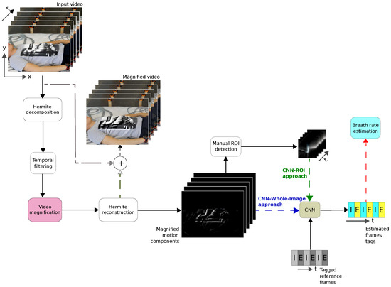
Figure 1. Block diagram of the breath rate estimation system showing the CNN-ROI and CNN-Whole-Image approaches.

2.2.1. Hermite Transform–Motion Magnification

In this work, we used an implementation of the Eulerian motion magnification method [22] through Hermite transform (HT) [32] to represent the spatial features of the image sequence. The Hermite transform description can be seen in Appendix A.

Following this, we present the Eulerian motion magnification basis, and we describe its implementation using Hermite transform.

Let $I(X,t)$ an image sequence, where $X={(x,y)}^{\top }$ represent the pixel position; $W\left(t\right)={\left({\delta }_x\left(t\right),{\delta }_y\left(t\right)\right)}^{\top }$ represents the corresponding displacements within the image domain and t is the time associated with each image in the sequence.

Thus, the intensities of pixel X on the image sequence can be expressed as a function of displacement $W\left(t\right)$:

$$I(X,t)=f\left(X+W\left(t\right)\right),$$

(1)

where $I(X,0)=f\left(X\right)$ is the first image of the sequence.

Applying the Hermite transform to Equation (1), we obtain a set of functions defined in terms of the displacement function $W\left(t\right)$ as shown in Equation (2):

$$I_{m,n-m}(X,t)=f_{m,n-m}\left(X+W\left(t\right)\right),$$

(2)

with $I_{m,n-m}(X,0)=f_{m,n-m}\left(X\right)$.

The Eulerian motion magnification method [22] consists of amplifying the displacement function $W\left(t\right)$ by a factor $\alpha$ to obtain a synthesized representation of the Hermite coefficients:

$${\widehat{I}}_{m,n-m}(X,t)=f_{m,n-m}\left(X+(1+\alpha )W\left(t\right)\right).$$

(3)

If we applied in Equation (2) a first-order Taylor decomposition to $I_{m,n-m}(X,t)$, we obtain:

$$I_{m,n-m}(X,t)\approx f_{m,n-m}\left(X\right)+W{\left(t\right)}^T(\nabla f_{m,n-m}\left(X\right)),$$

(4)

where ∇ represents the gradient operator and $W{\left(t\right)}^T(\nabla f_{m,n-m}\left(X\right))$ represents the high-order terms of the Taylor expansion, i.e., the motion components of the Hermite coefficients.

Next, we applied a broadband temporal band filter to Equation (4) to retain the displacement vector $W\left(t\right)$ obtaining:

$$B_{m,n-m}(X,t)=W{\left(t\right)}^T(\nabla f_{m,n-m}\left(X\right)).$$

(5)

Multiplying $B_{m,n-m}(X,t)$ by the factor $\alpha$ and summing it to $I_{m,n-m}(X,t)$ we obtain:

$${\tilde{I}}_{m,n-m}(X,t)=I_{m,n-m}(X,t)+\alpha \left(W{\left(t\right)}^T(\nabla f_{m,n-m}\left(X\right))\right).$$

(6)

Replacing $I_{m,n-m}$ in Equation (6) by the Taylor expansion of Equation (4) we obtain:

$$\begin{array}{cc}\hfill {\tilde{I}}_{m,n-m}(X,t)& \approx f_{m,n-m}\left(X\right)+W{\left(t\right)}^T\left(\nabla f_{m,n-m}\left(X\right)\right)+\alpha \left(W{\left(t\right)}^T(\nabla f_{m,n-m}\left(X\right))\right)\hfill \\ \hfill & \approx f_{m,n-m}\left(X\right)+W{\left(t\right)}^T(1+\alpha )\left(\nabla f_{m,n-m}\left(X\right)\right).\hfill \end{array}$$

(7)

We can demonstrate that if the first-order Taylor series holds in Equation (7), the amplification of the temporal bandpass signal $B_{m,n-m}(X,t)$ is related to the motion amplification of Equation (3):

$${\tilde{I}}_{m,n-m}(X,t)\approx f_{m,n-m}\left(X+(1+\alpha )W\left(t\right)\right).$$

(8)

Finally, the motion magnification sequence $\tilde{I}(X,t)$ can be obtained by applying the inverse Hermite transform to Equation (8) (see Appendix A):

$$\tilde{I}(X,t)=\sum _n^{\infty }\sum _{m=0}^n\sum _{\left(X_0\right)\in S}{\tilde{I}}_{m,n-m}(X_0,t)·P_{m,n-m}(X-X_0)$$

(9)

In practical terms, instead of summing the magnified spatial components and then performing the inverse Hermite transform, we can interchange it and first perform the reconstruction of the magnified spatial components and then sum it with the original image. This is because the inverse Hermite transform (Equation (A4)) and the motion magnification technique (Equation (6)) are both linear processes.

The Eulerian motion magnification proposal used in this work can be summarized as follows:

• Carry out a spatial decomposition of the image sequence using Hermite transform. This allows decomposition of the image sequence into different spatial frequency bands that are related with different motions (see Equation (4))
• Perform a temporal filtering of the spatial decomposition to retain the motion components (Equation (5)). The cut frequencies of the filter are chosen to retain the motions components depending the application. In this case, the cut frequencies are related to the human respiratory frequencies.
• Amplify the different spatial frequency bands by the $\alpha$ factor.
• Reconstruct the magnified motion components through an inverse spatial decomposition process (inverse Hermite transform).
• Add the reconstructed magnified motion components to the original image sequence by means of (Equation (6)).

In Figure 2 we show some reconstructed images by using the magnified motion components ($\alpha B(X,t)$) before summing it to the original image sequence, where the reconstructed images correspond to inhalation (‘I’) and exhalation (‘E’) frames. Later, the reconstructed magnified motion component images will be used as input to the CNN net.

Figure 2. Reconstructed images using the magnified motion components from the image sequence showing some respiratory phases. (a,c,e,g,i) Frames representing the inhalation ‘I’ phase. (b,d,f,h,j) Frames representing the exhalation ‘E’ phase.

2.2.2. Convolutional Neural Networks

CNNs are nets inspired on the nature of visual perception in living creatures mainly applied for image processing [35,36]. There exist different topologies which include two basic steps: feature extraction and classification model. In the feature extraction step, several neural layers are employed such as convolutional and pooling. A convolutional layer aims to compute feature representations of the input, a pooling layer aims to reduce the resolution of feature maps. In the classification model step, dense networks are the most used ones that include a fully connected layer that aims to perform high-level reasoning. In addition, for classification purposes a SoftMax layer is mainly implemented at the end of the network [36].

We propose a CNN that receives an input image of the video magnification and returns an output class representing ‘I’ or ‘E’, as shown in Figure 2. The input image is resized to the fixed dimensions $28\times 28$ pixels. The topology of the CNN consists of: an input layer that receives a grayscale image, a convolutional layer with 25 filters of size $12\times 12$ with a rectified linear unit (ReLU); then, there is a 2-size fully connected layer that feeds a SoftMax layer; and finally, a classification layer is occupied to compute the corresponding output class. Finally, we obtained a temporal vector labeled in each frame position as ‘I’ or ‘E’. In Figure 3 we show the topology of the CNN including the two strategies for training the network: the CNN-ROI and CNN-Whole-Image approaches.

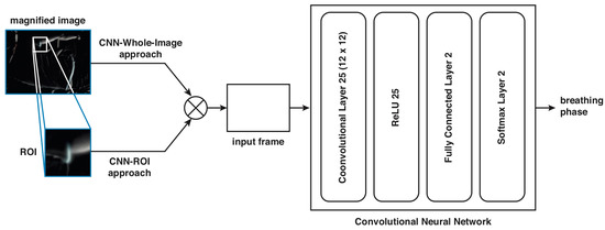
Figure 3. CNN-topology for detecting the two phases of breathing: inhalation (‘I’) or exhalation (‘E’).

2.2.3. Respiratory Rate Estimation

The proposed respiratory rate measuring system is based on motion magnification technique using Hermite transform and a CNN to classify the frames. Respiratory rate estimation is computed using the method proposed by [30] as explained next.

Once the CNN classifies each frame in the image sequence, and it is assigned a label inhalation (‘I’) or exhalation (‘E’), a binary vector $A=\left[A\right(1),A(2),\dots ,A(N\left)\right]$ is formed where for each one of the frames the label ‘I’ is changed by ‘1’ and the label ‘E’ by ‘0’, and N corresponds to the number of frames of the video. In Figure 4 we show an example of the binary vector A.

Figure 4. Example of the distances computed (number of frames) for an inhalation–exhalation cycle to form the binary vector A, each color represents a different cycle.

Next, we measure the distances (in number of frames) $D\left(k\right)$ that the signal takes to complete each one of the breathing cycles (see Figure 4), e.g., from inhalation (‘1’) to exhalation (‘0’), and we calculated an average distance $D_{mean}$ as follows:

$$D_{mean}=\frac{1}{p}\sum _{k=1}^{p}D\left(k\right),$$

(10)

where p is the number of $D\left(k\right)$ calculated distances.

Finally, the breath rate $RR$ (in bpm) is calculated using Equation (11):

$$RR=\frac{\left(60\right)\left(N\right)}{\left(T\right)\left(D_{mean}\right)},$$

(11)

where T is the duration in seconds of the video.

2.3. Experimentation

2.3.1. Parameters Setting

Before applying the Hermite transform–motion magnification method to the datasets, the following parameters must be defined: the size of the Gaussian window, the order maximum of the spatial decomposition, the cutting frequencies in the temporal filtering, and the amplification factor used.

In Appendix A.1, we present the suitable values to the Gaussian window and consequently, the maximum expansion order $2\mathcal{N}$ of the Hermite transform; thus, to avoid the blur artifacts in the reconstruction step, we used a Gaussian window of $5\times 5$ pixels ($\mathcal{N}=4$), which allows us a maximum order of the expansion of 8 ($2\mathcal{N}=2\times 4$) giving a perfect reconstruction of the image sequence. A Gaussian window of $3\times 3$ pixels ($\mathcal{N}=2$) also would avoid the blurring effect in the edges but would limit the expansion order to 4, giving a less quality of the reconstructed images.

On the other hand, in [37] was presented a multi-resolution version of the Hermite transform, which allows us to analyze the spatial structures in the image at different scales. This multi-resolution analysis is independent to the reconstruction process, whence we performed a spatial decomposition of 8 levels of resolution with a sub-sampling factor of 2 without affecting of the quality of the reconstructed image sequence.

For motion magnification, we applied a temporal band pass filter to the Hermite coefficients through the difference of two IIR (Infinite Impulse Response) low-pass filter as in [22], where the cutting frequencies for the band pass filter were fixed to 0.15–0.4 Hz corresponding to 9–24 breaths per minute. This range is sufficient to detect breathing rate in healthy subjects at rest.

The amplification factor $\alpha$ was set to 20, in such a way that allowed effortlessly seeing the respiratory movements in the thorax. In Appendix B, we describe the value limit of the amplification factor, the relation of it with the spatial wavelength of the image sequence, and how it is applied in each level of the spatial decomposition.

For the approach including a ROI, the user selects a point in the thoracic region, and a window of size ($48\times 64$ pixels ) centered in the selected point is created, the size of the ROI window must be equal or higher to $28\times 28$ pixels, since the CNN resizes the input images to correspond with $28\times 28$ pixels. The size of the original frame video, as mentioned above, is $480\times 640$ pixels. The size of the ROI was chosen experimentally but in relation to the distance of the camera and the spatial resolution. In this case the size of the ROI is $\frac{1}{10}$ of the size of the image frame. This manual strategy allows choice of a zone including the thoracic area where its motion is clearly appreciated facilitating in this way the classification to the algorithm.

2.3.2. Experiment Settings

Two kinds of experiments were carried out: the CNN-ROI proposal using 5 trials (5 subjects in ‘LD’ position) and the CNN-whole-image proposal using 25 trials (ten subjects, 6 in ‘LU’ position, 8 in ‘LD’ position, 6 in ‘LF’ position and 5 in ‘S’ position). For this last experiment, we tested three different approaches for detecting the two phases of breathing: (i) using the original video without any processing, (ii) using the magnification component video, and (iii) using the magnification video, i.e., original video added to the magnification components.

In the two experiments, we develop a CNN-model using the information of all the subjects (depending of the experiment), splitting data in 70% training and 30% testing sets. For implementation purposes, we trained the CNN using the stochastic gradient descent algorithm with initial learning rate of 1E-6, regularization coefficient of 1E-4, maximum number of epochs 200, and mini-batch size of 128. The binary classification response (inhalation/exhalation) of the CNN is evaluated using the accuracy metric as shown in Equation (12), where $TP$ and $TN$ are the true positives and true negatives, and $FP$ and $FN$ are the false positives and false negatives.

$$accuracy=\frac{TP+TN}{TP+TN+FP+FN}$$

(12)

For the two approaches, we compute the Mean Absolute Error (MAE) to evaluate the estimation of the RR as:

$$MAE=\frac{\parallel R{R}_{ref}-RR\parallel }{R{R}_{ref}}\times 100$$

(13)

The reference $R{R}_{ref}$ was obtained visually from the magnified video.

3. Results

3.1. Training of Convolutional Neural Networks

For the CNN-ROI proposal the dataset was split in 70% training (7867 samples) and 30% (3372 samples) testing sets. Table 2 shows the evaluation results when testing ROI images as inputs to the CNN-model. As shown, the accuracy obtained was $98.42\pm 0.173\%$ (mean ± standard deviation), representing that $98\%$ of the time the estimation is the same as the targets.

Table 2. Performance results for the CNN-ROI proposal.

Subject	Accuracy (%)
2	98.25
3	98.35
5	98.30
7	98.56
8	98.65
Mean	98.42
SD	$\pm 0.173$

For the CNN-whole-image proposal, we tested three different approaches for detecting the two phases of breathing, depending on the input images to the CNN: (i) the CNN-model with original video (OV) without processing, (ii) the CNN-model with the reconstructed magnified components video (MCV), and (iii) the CNN-model with the magnified video (MV). In the three cases, we split the data into a 70% training set (34,660) and a 30% (14,854) testing set. Table 3 summarizes the performance of the CNN models using the testing set, where the subject and his/her pose are listed in the first two columns. As shown, the least accurate CNN-model corresponds to the one using the original video without any processing ($83.33\pm 4.92\%$ for OV approach) while the other two approaches look similar in response ($97.30\pm 1.32\%$ for MCV approach and $97.66\pm 1.26\%$ for MV approach).

Table 3. Accuracy results of the CNN, in testing, using different approaches.

Subject	Pose	OV Video (%)	MCV (%)	MV (%)
1	LU	81.36	94.13	93.54
1	LF	80.79	97.86	98.41
2	LD	76.77	97.92	98.88
3	LD	84.25	97.48	97.86
3	S	92.87	98.01	98.40
4	LU	88.46	98.05	98.57
4	LF	79.75	97.27	97.43
4	LD	76.44	98.11	98.46
4	S	85.24	97.71	98.15
5	LU	87.49	96.94	97.16
5	LD	78.42	98.35	97.97
5	S	76.57	97.54	97.54
6	LU	79.43	93.16	94.09
6	LD	80.09	95.10	97.03
7	LU	92.33	98.12	98.57
7	LF	87.53	98.63	98.21
7	LD	85.37	97.23	98.34
7	S	93.41	98.30	99.34
8	LU	84.56	96.04	97.85
8	LF	80.33	97.76	98.09
8	LD	84.06	98.27	98.33
8	S	81.34	97.32	97.65
9	LF	80.40	97.03	97.40
9	LD	80.20	98.28	98.50
9	S	87.33	97.65	97.77
10	LF	81.86	97.62	97.62
Mean		83.33	97.30	97.66
SD		$\pm 4.92$	$\pm 1.32$	$\pm 1.26$

3.2. Respiratory Rate Estimation Using CNN-ROI

We compared the CNN-ROI method with the IPM proposal [29]. For details of the IPM method see [29,30].

Results of the RR estimation in breaths per minute (bpm) are shown in Table 4. It shows the respiratory rate estimation from the five subjects. In column one, the subject is displayed, in column two the ground-truth of respiratory rate, in column three and four the respiratory rate estimation using the CNN estimation method and the associated error in percentage. In column five and six the respiratory rate estimation and the associated error using the IPM method is displayed. The mean average error (MAE) obtained by the CNN proposal is $1.830\pm 1.610\%$ and MAE obtained by the IPM method is $2.470\pm 2.300\%$. Bland–Altman analysis was carried out for our CNN-ROI approach obtaining a MOD of 0.163 and LOAs of +1.01 and −0.68. The $95\%$ of limits of agreements were defined as the mean difference $\pm 1.96\sigma$, where $\sigma$ is the standard deviation of the differences. The bias is then $0.16\pm 0.85$ bpm ($\mathrm{MOD}\pm 1.96\sigma$), $\mathrm{PCC}=0.99$, $\mathrm{SCC}=0.91$ and $\mathrm{RMSE}=0.41$ as shown in Table 5.

Table 4. Results of respiratory rate estimation (bpm) using the CNN-ROI proposal.

Subject	Ref.	CNN	Err. CNN (%)	IPM	Err. IPM (%)
2	15	15.009	0.06	15.153	1.002
3	21	20.678	1.533	22.320	6.285
5	13	13.453	3.366	13.270	2.034
7	13	12.926	0.569	12.957	0.386
8	20	20.752	3.625	20.545	2.629
Mean	16.42	16.56	1.83	16.84	2.47
SD	$\pm 3.84$	$\pm 3.86$	$\pm 1.61$	$\pm 4.31$	$\pm 2.30$

Table 5. Metrics quality to evaluate the estimation of the RR.

	RMSE (bpm)	MAE (bpm)	MAE (%)	MOD (bpm)	LOAs (bpm)	$\mathbf{MOD}\pm 1.96\mathit{\sigma }$ (bpm)	SCC, PCC
Brieva et al. [29]	-	-	$2.47\pm 2.30$	-	-	-	-
Massaroni et al. [20]	-	$0.39$	-	$-0.01$	$+1$, $-1.02$	$-0.01\pm 1.01$	-
Al-Naji et al. [30]	-	-	1.314	$0.21$	$+0.88$, $-0.46$	$0.21\pm 0.67$	$0.956$, $0.966$
Ganfure [24]	-	-	$15.34$	-	-	-	-
Alinovi et al. [25]	$0.05$	-	-	-	-	-	-
Alam et al [26]	-	-	$20.11$	-	-	-	-
Chen et al. [18]	-	$3.02$	-	-	-	-	-
Our proposal using ROI	$0.41$	$0.32$	$1.83\pm 1.61$	$0.16$	$+1.01$, $-0.68$	$0.16\pm 0.85$	$0.91$, $0.99$
Our proposal without ROI	$0.85$	$0.56$	$3.28\pm 3.33$	$0.347$	$+1.8$, $-1.1$	$0.347\pm 1.45$	$0.975$, $0.977$

3.3. Respiratory Rate Estimation Using CNN-Whole-Image

In Figure 5, we show the tagged results obtained for each approach with Trial 1 of Patient 7 in ‘LF’ position. The first row shows the tagged reference, where the x-axis indicates the frame number where the breathing changes from inhalation (‘I’) to exhalation (‘E’) or vice versa. The next rows show the tagged estimation for each approach, where both the MVC and MV approaches overcome the approach that uses the original video as input to the CNN.

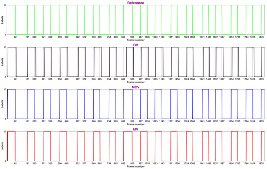
Figure 5. Tagged results obtained for the trial 1 of patient 7 in ‘LF’ position.

Later, we applied Equation (11) to the estimated temporal vectors obtained from the CNN. Results of this process are summarized in Table 6. The subject and the pose are listed in the first and second columns, respectively. Then, in columns three, four and five the estimations of RR from the reconstructed magnified components video (MCV) as input, the magnified video (MV) as input and the original video (OV) as input, respectively, are shown. Then, the reference RR for each subject is reported in column six. After that, it is the MAE for the three approaches in columns seven, eight, and nine. The MEA obtained by the CNN-Whole-Image proposal in the three approaches are $3.28\pm 3.33$ for the MCV, $3.15\pm 5.04$ for the MV and $6.84\pm 9,79$ for the OV. The MAE obtained using the MCV strategy for different positions of the subject are: for the ‘LD’ position $2.14\pm 1.17\%$, for the ‘S’ position $1.51\pm 1.10\%$, for the ‘LU’ position $6.14\pm 4.21\%$ and for ‘LF’ position $4.63\pm 4.51\%$.

Table 6. Error (bpm) of the CNN-whole-image proposal using the three approaches.

S	Pose	RR MCV	RR MV	RR OV	RR Reference	MCV %	MV %	OV %
1	LU	21.2	24.08	21.65	19	11.579	26.737	13.947
1	LF	13.243	13.235	19.388	13	1.869	1.808	49.138
2	LD	15.367	15.358	14.041	15	2.447	2.387	6.393
3	LD	20.69	20.69	20.442	21	1.476	1.476	2.657
3	S	17.024	17.045	16.092	17	0.141	0.265	5.341
4	LD	17.387	17.459	16.422	17	2.276	2.700	3.400
4	LU	13.664	13.699	13.623	14	2.400	2.150	2.693
4	LF	18.859	17.811	17.067	18	4.772	1.050	5.183
4	S	21.563	21.976	21.451	22	1.986	0.109	2.495
5	LD	13.44	13.419	14.279	13	3.385	3.223	9.838
5	LU	10.49	10.508	10.514	11	4.636	4.473	4.418
5	S	14.086	14.055	14.063	14	0.614	0.393	0.450
6	LD	18.912	18.728	18.761	19	0.463	1.432	1.258
6	LF	20.432	18.905	13.969	18	13.511	5.028	22.394
7	LD	12.911	12.911	12.05	13	0.685	0.685	7.308
7	LU	14.251	13.195	13.579	13	9.623	1.500	4.454
7	LF	15.634	16.311	15.376	16	2.288	1.944	3.900
7	S	15.162	15.135	15.162	15	1.080	0.900	1.080
8	LD	20.715	19.344	19.054	20	3.575	3.280	4.730
8	LU	20.499	21.2	19.042	20	2.495	6.000	4.790
8	LF	22.835	22.898	24.098	22	3.795	4.082	9.536
8	S	21.453	21.526	20.385	21	2.157	2.505	2.929
9	LD	18.445	18.462	18.388	19	2.921	2.832	3.221
9	LF	18.284	18.254	18.388	18	1.578	1.411	2.156
9	S	21.659	21.649	21.669	21	3.138	3.090	3.186
10	LF	15.929	15.91	15.817	16	0.444	0.562	1.144
Mean		17.46	17.45	17.10	17.11	3.28	3.15	6.84
SD		$\pm 3.42$	$\pm 3.59$	$\pm 3.40$	$\pm 3.21$	$\pm 3.33$	$\pm 5.04$	$\pm 9.79$

The Bland–Altman method was used to assess the level of agreement between the experimental results obtained from the proposed system and those obtained from the reference. The $95\%$ of limits of agreements were defined as MOD $\pm 1.96\sigma$, where $\sigma$ is the standard deviation of the differences. The bias is then MOD $\pm 1.96\sigma$. In addition, the relationship between the estimated values and the reference was evaluated using Pearson’s correlation coefficient (PCC), the Spearman correlation coefficient (SCC) and the root mean square error (RMSE). The Bland–Altman plots and the statistics for RR measurements based on our CNN-whole-image proposal are shown in Figure 6. This was obtained for the MCV strategy a MOD of $0.347$ with limits of agreement of $+1.8$ and $-1.10$ corresponding to a bias of $0.347\pm 1.45\mathrm{bpm}$ with statistics $\mathrm{PCC}=0.977$, $\mathrm{SCC}=0.975$ and $\mathrm{RMSE}=0.805$ as shown in Table 5. For the MV strategy a MOD of $0.33$ was obtained with limits of agreement of $+2.43$ and $-1.76$ corresponding to a bias of $0.33\pm 2.1$ bpm and statistics $\mathrm{PCC}=0.956$, $\mathrm{SCC}=0.965$ and $\mathrm{RMSE}=1.1$. Finally, for the OV strategy, a MOD of $-0.01$ was obtained with limits of agreement or $+3.469$ and $-3.496$ corresponding to a bias of $-0.01\pm 3.468$ bpm and statistics $\mathrm{SCC}=0.836$, $\mathrm{PCC}=0.858$ and $\mathrm{RMSE}=1.74$. When the results are compared between the three strategies, with the use of the MCV strategy, the higher correlation ($\mathrm{PCC}=0.977$, $\mathrm{SCC}=0.975$) is obtained, along with the smallest error ($\mathrm{RMSE}=0.805$) and the least limits of agreement ($+1.8$ and $-1.10$). Concerning the position of the subject, using the MCV strategy, a MOD of $0.157$ was obtained for the Bland–Altman analysis and the statistics for the ‘S’ position, with limits of agreement of $+0.899$ and $-0.583$ corresponding to a bias of $0.157\pm 0.742$ bpm with statistics $\mathrm{SCC}=0.910$, $\mathrm{PCC}=0.994$, $\mathrm{RMSE}=0.38$; for the ‘LD’ position a MOD of $0.108$ with limits of agreement of $+0.957$ and $-0.741$ corresponding to a bias of $0.108\pm 0.84$ bpm with statistics $\mathrm{SCC}=0.964$, $\mathrm{PCC}=0.991$ and $\mathrm{RMSE}=0.42$; for the ‘LU’ position a MOD of $0.620$ with limits of agreement of $+2.834$ and $-1.592$ corresponding to a bias of $0.620\pm 2.21$ bpm with statistics $\mathrm{SCC}=0.91$, $\mathrm{PCC}=0.98$ and $\mathrm{RMSE}=1.19$ and for the ‘F’ position a MOD of $0.602$ with limits of agreement of $+2.407$ and $-1.203$ corresponding to a bias of $0.602\pm 1.8$ bpm and statistics $\mathrm{SCC}=0.954$, $\mathrm{PCC}=0.965$ and $\mathrm{RMSE}=1.04$. The Bland–Altman plots and the statistics are shown in Figure 7. It is observed that the less RMSE, the less limits of agreements are obtained for the ‘S’ position ($\mathrm{RMSE}=0.38$, $+2.407$, $-1.203$) and the ‘LD’ position ($\mathrm{RMSE}=0.42$, $+2.407$, $-1.203$).

Figure 6. Bland–Altman plot obtained considering all the subjects: black line is the MOD, red lines are the LOAs. (a) Using the original video. (b) Using the magnified video. (c) Using the reconstructed motion components.

Figure 7. Bland–Altman plot obtained for each position: black line is the bias, red lines are the Limits of agreements. (a) ‘LD’ position. (b) ‘LU’ position. (c) ‘S’ position. (d) ‘F’ position.

4. Discussion

The proposed system succeeded in measuring RR for subjects at rest in different positions. In Table 5 the quality metrics used in the reviewed works and in our proposal are shown. It is clear that using the MCV strategy, estimation was in close agreement (≈98%, $\mathrm{bias}=0.347\pm 1.45\mathrm{bpm}$) with the reference obtained by visual counting in contrast to the MV, where the agreement fell to ≈97% ($\mathrm{bias}=0.33\pm 2.1\mathrm{bpm}$) and to the OV strategy, where the agreement fell to ≈96% ($\mathrm{bias}=-0.01\pm 3.468\mathrm{bpm}$). Hence, it is observed that the difference error with respect to the reference based on the MCV strategy fell to $<\pm 2$ bpm with a MAE of $3.28\pm 3.33\%$ while the MV strategy fell to $<\pm 3$ bpm with a MAE of $3.15\pm 5.05\%$ and the OV strategy fell to $<\pm 4$ bpm a MAE of $6.84\pm 9.79\%$. We observe then that the use of the magnification process and particularly the use of magnifying components instead of the original video or the magnified video improves detection. The use of the magnification process can produce artifacts in the video, but if we take only the magnified components, the presence of these artifacts is minimized. Concerning the position of the subject using the MCV strategy, the results were in close agreement for the ‘S’ position (≈99%, $\mathrm{bias}=0.157\pm 0.742\mathrm{bpm}$) and ‘LD’ position (≈99%, $\mathrm{bias}=0.108\pm 0.84\mathrm{bpm}$) and fall for ‘F’ position (≈98%, $\mathrm{bias}=0.602\pm 1.80\mathrm{bpm}$) and ‘LU’ position (≈97 %, $\mathrm{bias}=0.620\pm 2.21\mathrm{bpm}$). These results confirm that our strategy can be used for different positions despite some variability in the agreement.

Compared to other recent works using Bland–Altman analysis, the work of Massaroni et al. [20] obtains an agreement of ≈98% ($\mathrm{bias}=-0.01\pm 1.01$) falling to a difference error with respect of the reference $<\pm 2$ bpm, consistent with our results. The work of Al-Naji et al. [30] obtains an agreement of ≈99% ($\mathrm{bias}=0.21\pm 0.62$) falling to a difference error with respect to the reference $<\pm 1$ bpm, consistent with our work. The two latter methods are dependent on the choice of the ROI in contrast to our CNN-Whole-Image strategy, which is independent of the choice of the ROI. In addition, our approach uses the tagged inhalation and exhalation frames as reference for training the CNN as opposed to other strategies that use a reference obtained by means of a contact standard sensor. Some reviewed works did not use the Bland–Altman analysis as quality metric to compare to other strategies. As shown in Table 5, Alinovi et al. [25] obtained a RMSE of 0.05 consistent value compared to our ROI strategy ($\mathrm{RMSE}=0.41$) and to our CNN-Whole-Image strategy ($\mathrm{RMSE}=0.85$). Alam et al. [26] proposed a method that did not need to use a ROI to obtain a MAE of 20.11% greater than our CNN-Whole-Image strategy with a MAE of $3.28\pm 3.33\%$. Ganfure et al. [24] proposed a method based on an automatic choosing of the ROI obtain a MAE of 15.4% greater than our two strategies. Finally, Chan et al. [18] obtained a MAE of 3.02 bpm greater than our ROI strategy ($\mathrm{MAE}=0.32\mathrm{bpm}$) and to our CNN-Whole-Image strategy ($\mathrm{MAE}=0.56\mathrm{bpm}$). Some of the limitations of this work are the limited number of subjects for the statistical analysis. The influence of the distance of the camera for all the tests was not studied. The influence of the kind of clothes of the participants, for example the use of a close-fit or loose-fit t-shirt, and the influence of some motions of the participant were not taken into account. Further strategies must be carried out to address these points. Our approach is simple to implement, using a basic CNN structure and requiring only the classification of the stages of the respiratory cycle. The conditions of acquisitions take into account not only the thorax area but the surrounding environment, thus it would work in some routine medical examinations where RR in controlled conditions is only required.In addition, we show that our CNN-Whole-Image strategy that did not need the selection of a ROI is competitive to all the strategies using a ROI.

5. Conclusions

In this work, we implemented a new non-contact strategy based on the Eulerian motion magnification technique using the Hermite transform and a CNN approach to estimate the respiratory rate. We implemented and tested two different strategies to estimate the respiratory rate, a CNN-ROI method that needs a manual ROI definition, and a CNN-Whole-Image strategy without requiring ROI. We proposed a CNN training method using the tagged inhalation and exhalation frames as reference. Our proposal, based on the CNN estimation, does not require any additional processing on the reconstructed sequence after the motion magnification instead of other video processing methods. The proposed system has been tested on healthy participants in different positions, in controlled conditions but taking into account the surroundings of the subject. The experimental results of the RR were successfully estimated at different positions obtaining a MAE for the automatic strategy of $3.28\pm 3.33$% agreement with respect to the reference of ≈98%. For future work we must test our approach in different kinds of scenarios, such as in the presence of some simple motions of the subject during acquisition, different camera distances, and different kind of clothes for the participants. This method can be tested for monitoring during longer periods of time.

Appendix A.1. The Discrete Hermite Transform

The expansion of the image sequence $I(X,t)$ of Equation (A2) requires convolution of the image at time t with an infinity set of Hermite filters $D_{m,n-m}$ with $n=0,\cdots ,\infty$, $m=0,\dots ,n$, in the discrete case, we limit the number of Hermite coefficients by [38]:

$$\begin{array}{cc}\hfill n& =0,\cdots ,2\mathcal{N}\hfill \\ \hfill m& =0,\dots ,n,\hfill \end{array}$$

(A7)

where $\mathcal{N}+1$ is the size of the Gaussian kernel, thus, the maximum order of the expansion is limited by the size of the discrete Gaussian window. For large values of $\mathcal{N}$ the discrete Gaussian kernel reduces to the Gaussian window.

Furthermore, instead of recovering the original image, we obtain an approximation of the original image $\widehat{I}(X,t)$, where the quality of this reconstruction improves by increasing the maximum order of the expansion $2\mathcal{N}$, i.e., the size of the Gaussian window $\mathcal{N}+1$ [38]. In terms of the artifacts in the approximated image $\widehat{I}(X,t)$, small values of the Gaussian windows causes “speckles”, while high values result in Gibbs-phenomenon-like artifacts such as ringing and blur [41].

Thus, to determine the maximum order or the expansion $2\mathcal{N}$ and consequently the size of the Gaussian window $\mathcal{N}+1$, in [41] van Dijk and Martens determined that using an expansion of the Hermite transform equal to 3, the reconstructed image will contain the largest quantity of AC energy ($84\%$) according to Parseval’s theorem. In general, with $2\mathcal{N}\ge 3$ we can obtain a good reconstruction and with much greater values we will obtain a perfect reconstruction of the image, e.g., $2\mathcal{N}=8$.

References

- Zhao, F.; Li, M.; Qian, Y.; Tsien, J. Remote Measurements of Heart and Respiration Rates for Telemedicine. PLoS ONE 2013, 8, e71384. [Google Scholar] [CrossRef] [PubMed]
- Massaroni, C.; Nicola, A.; Lo Presti, D.; Sacchetti, M.; Silvestri, S.; Schena, E. Contact-Based Methods for Measuring Respiratory Rate. Sensors 2019, 19, 908. [Google Scholar] [CrossRef] [PubMed]
- Al-Naji, A.; Gibson, K.; Lee, S.H.; Chahl, J. Monitoring of Cardiorespiratory Signal: Principles of Remote Measurements and Review of Methods. IEEE Access 2017, 5, 15776–15790. [Google Scholar] [CrossRef]
- Li, C.; Chen, F.; Jin, J.; Lv, H.; Li, S.; Lu, G.; Wang, J. A method for remotely sensing vital signs of human subjects outdoors. Sensors 2015, 15, 14830–14844. [Google Scholar] [CrossRef] [PubMed]
- Lee, Y.; Pathirana, P.; Evans, R.; Steinfort, C. Noncontact detection and analysis of respiratory function using microwave Doppler Radar. J. Sens. 2015, 2015. [Google Scholar] [CrossRef]
- Dafna, E.; Rosenwein, T.; Tarasiuk, A.; Zigel, Y. Breathing rate estimation during sleep using audio signal analysis. In Proceedings of the 2015 37th Annual International Conference of the IEEE Engineering in Medicine and Biology Society (EMBC), Milan, Italy, 25–29 August 2015; Volume 2015, pp. 5981–5984. [Google Scholar] [CrossRef]
- Min, S.; Kim, J.; Shin, H.; Yun, Y.; Lee, C.; Lee, M. Noncontact respiration rate measurement system using an ultrasonic proximity sensor. IEEE Sens. J. 2010, 10, 1732–1739. [Google Scholar] [CrossRef]
- Massaroni, C.; Venanzi, C.; Silvatti, A.P.; Lo Presti, D.; Saccomandi, P.; Formica, D.; Giurazza, F.; Caponero, M.A.; Schena, E. Smart textile for respiratory monitoring and thoraco-abdominal motion pattern evaluation. J. Biophotonics 2018, 11, e201700263. [Google Scholar] [CrossRef]
- Mutlu, K.; Rabell, J.; Martin del Olmo, P.; Haesler, S. IR thermography-based monitoring of respiration phase without image segmentation. J. Neurosci. Methods 2018, 301, 1–8. [Google Scholar] [CrossRef]
- Schoun, B.; Transue, S.; Choi, M.H. Real-time Thermal Medium-based Breathing Analysis with Python. In Proceedings of the 7th Workshop on Python for High-Performance and Scientific Computing, New York, NY, USA, 13–16 November 2017. [Google Scholar] [CrossRef]
- Nguyen, V.; Javaid, A.; Weitnauer, M. Detection of motion and posture change using an IR-UWB radar. In Proceedings of the 7th Workshop on Python for High-Performance and Scientific Computing, Salt Lake City, Utah, 13–18 November 2016; Volume 2016, pp. 3650–3653. [Google Scholar] [CrossRef]
- Moreno, J.; Ramos-Castro, J.; Movellan, J.; Parrado, E.; Rodas, G.; Capdevila, L. Facial video-based photoplethysmography to detect HRV at rest. Int. J. Sport. Med. 2015, 36, 474–480. [Google Scholar] [CrossRef]
- Tarassenko, L.; Villarroel, M.; Guazzi, A.; Jorge, J.; Clifton, D.A.; Pugh, C. Non-contact video-based vital sign monitoring using ambient light and auto-regressive models. Physiol. Meas. 2014, 35, 807–831. [Google Scholar] [CrossRef]
- Van Gastel, M.; Stuijk, S.; De Haan, G. Robust respiration detection from remote photoplethysmography. Biomed. Opt. Express 2016, 7, 4941–4957. [Google Scholar] [CrossRef] [PubMed]
- Nilsson, L.; Johansson, A.; Kalman, S. Monitoring of respiratory rate in postoperative care using a new photoplethysmographic technique. J. Clin. Monit. Comput. 2000, 16, 309–315. [Google Scholar] [CrossRef] [PubMed]
- L’Her, E.; N’Guyen, Q.T.; Pateau, V.; Bodenes, L.; Lellouche, F. Photoplethysmographic determination of the respiratory rate in acutely ill patients: Validation of a new algorithm and implementation into a biomedical device. Ann. Intensive Care 2019, 9. [Google Scholar] [CrossRef] [PubMed]
- Bousefsaf, F.; Maaoui, C.; Pruski, A. Continuous wavelet filtering on webcam photoplethysmographic signals to remotely assess the instantaneous heart rate. Biomed. Signal Process. Control 2013, 8, 568–574. [Google Scholar] [CrossRef]
- Chen, W.; McDuff, D. DeepPhys: Video-Based Physiological Measurement Using Convolutional Attention Networks. Lect. Notes Comput. Sci. 2018, 11206 LNCS, 356–373. [Google Scholar] [CrossRef]
- Al-Naji, A.; Chahl, J. Simultaneous Tracking of Cardiorespiratory Signals for Multiple Persons Using a Machine Vision System With Noise Artifact Removal. IEEE J. Transl. Eng. Health Med. 2017, 5, 1–10. [Google Scholar] [CrossRef] [PubMed]
- Massaroni, C.; Lo Presti, D.; Formica, D.; Silvestri, S.; Schena, E. Non-Contact Monitoring of Breathing Pattern and Respiratory Rate via RGB Signal Measurement. Sensors 2019, 19, 2758. [Google Scholar] [CrossRef]
- Liu, C.; Yang, Y.; Tsow, F.; Shao, D.; Tao, N. Noncontact spirometry with a webcam. J. Biomed. Opt. 2017, 22, 1–8. [Google Scholar] [CrossRef]
- Wu, H.Y.; Rubinstein, M.; Shih, E.; Guttag, J.; Durand, F.; Freeman, W.T. Eulerian Video Magnification for Revealing Subtle Changes in the World. ACM Trans. Graph. 2012, 31, 1–8. [Google Scholar] [CrossRef]
- Al-Naji, A.; Gibson, K.; Chahl, J. Remote sensing of physiological signs using a machine vision system. J. Med. Eng. Technol. 2017, 41, 396–405. [Google Scholar] [CrossRef]
- Ganfure, G. Using video stream for continuous monitoring of breathing rate for general setting. Signal Image Video Process. 2019. [Google Scholar] [CrossRef]
- Alinovi, D.; Ferrari, G.; Pisani, F.; Raheli, R. Respiratory rate monitoring by video processing using local motion magnification. In Proceedings of the 2018 26th European Signal Processing Conference (EUSIPCO), Rome, Italy, 3–7 September 2018; Volume 2018, pp. 1780–1784. [Google Scholar] [CrossRef]
- Alam, S.; Singh, S.; Abeyratne, U. Considerations of handheld respiratory rate estimation via a stabilized Video Magnification approach. In Proceedings of the 2017 39th Annual International Conference of the IEEE Engineering in Medicine and Biology Society (EMBC), Seogwipo, South Korea, 11–15 July 2017; pp. 4293–4296. [Google Scholar] [CrossRef]
- Brieva, J.; Moya-Albor, E.; Gomez-Coronel, S.; Ponce, H. Video motion magnification for monitoring of vital signals using a perceptual model. In Proceedings of the 12th International Symposium on Medical Information Processing and Analysis, Tandil, Argentina, 5–7 December 2017; Volume 10160. [Google Scholar]
- Deng, F.; Dong, J.; Wang, X.; Fang, Y.; Liu, Y.; Yu, Z.; Liu, J.; Chen, F. Design and Implementation of a Noncontact Sleep Monitoring System Using Infrared Cameras and Motion Sensor. IEEE Trans. Instrum. Meas. 2018, 67, 1555–1563. [Google Scholar] [CrossRef]
- Brieva, J.; Moya-Albor, E.; Rivas-Scott, O.; Ponce, H. Non-contact breathing rate monitoring system based on a Hermite video magnification technique. OPENAIRE 2018, 10975. [Google Scholar] [CrossRef]
- Al-Naji, A.; Chahl, J. Remote respiratory monitoring system based on developing motion magnification technique. Biomed. Signal Process. Control 2016, 29, 1–10. [Google Scholar] [CrossRef]
- Brieva, J.; Moya-Albor, E. Phase-based motion magnification video for monitoring of vital signals using the Hermite transform. Med. Inf. Process. Anal. 2017, 10572. [Google Scholar] [CrossRef]
- Brieva, J.; Moya-Albor, E.; Gomez-Coronel, S.L.; Escalante-Ramírez, B.; Ponce, H.; Mora Esquivel, J.I. Motion magnification using the Hermite transform. In Proceedings of the 11th International Symposium on Medical Information Processing and Analysis, Cuenca, Ecuador, 17–19 November 2015; Volume 9681, pp. 96810Q–96810Q-10. [Google Scholar] [CrossRef]
- Altman, D.G.; Bland, J.M. Measurement in Medicine: The Analysis of Method Comparison Studies. J. R. Stat. Soc. Ser. D 1983, 32, 307–317. [Google Scholar] [CrossRef]
- Janssen, R.; Wang, W.; Moço, A.; de Haan, G. Video-based respiration monitoring with automatic region of interest detection. Physiol. Meas. 2015, 37, 100–114. [Google Scholar] [CrossRef]
- Nogueira, K.; Penatti, O.; dos Santos, J. Towards better exploiting convolutional neural networks for remote sensing scene classification. Pattern Recognit. 2017, 61, 539–556. [Google Scholar] [CrossRef]
- Gu, J.; Wang, Z.; Kuen, J.; Ma, L.; Shahroudy, A.; Shuai, B.; Liu, T.; Wang, X.; Wang, G.; Cai, J.; et al. Recent advances in convolutional neural networks. Pattern Recognit. 2017, 2017, 1–24. [Google Scholar] [CrossRef]
- Escalante-Ramírez, B.; Silván-Cárdenas, J.L. Advanced modeling of visual information processing: A multiresolution directional-oriented image transform based on Gaussian derivatives. Signal Process. Image Commun. 2005, 20, 801–812. [Google Scholar] [CrossRef]
- Martens, J.B. The Hermite Transform-Theory. IEEE Trans. Acoust. Speech Signal Process. 1990, 38, 1595–1606. [Google Scholar] [CrossRef]
- Martens, J.B. The Hermite Transform-Applications. IEEE Trans. Acoust. Speech Signal Process. 1990, 38, 1607–1618. [Google Scholar] [CrossRef]
- Sakitt, B.; Barlow, H.B. A model for the economical encoding of the visual image in cerebral cortex. Biol. Cybern. 1982, 43, 97–108. [Google Scholar] [CrossRef] [PubMed]
- Van Dijk, A.M.; Martens, J.B. Image representation and compression with steered Hermite transforms. Signal Process. 1997, 56, 1–16. [Google Scholar] [CrossRef]
© 2020 by the authors. Licensee MDPI, Basel, Switzerland. This article is an open access article distributed under the terms and conditions of the Creative Commons Attribution (CC BY) license (http://creativecommons.org/licenses/by/4.0/).