Article

Fast Reaction to Sudden Concept Drift in the Absence of Class Labels

1
Computer Science and Information Technology, La Trobe University, Bundoora VIC 3086, Australia
2
Faculty of Information Technology, Monash University, Clayton 3800, Australia
*
Author to whom correspondence should be addressed.
Appl. Sci. 2020, 10(2), 606; https://doi.org/10.3390/app10020606
Submission received: 28 October 2019 / Revised: 12 December 2019 / Accepted: 8 January 2020 / Published: 14 January 2020
(This article belongs to the Section Computing and Artificial Intelligence)

Abstract

:

Featured Application

The proposed drift detector can be applied in areas such as intrusion detection, fraud detectors or monitoring and forecasting traffic.

Abstract

A data stream can be considered as a sequence of examples that arrive continuously and are potentially unbounded, such as web page visits, sensor readings and call records. One of the serious and challenging problems that appears in a data stream is concept drift. This problem occurs when the relation between the input data and the target variable changes over time. Most existing works make an optimistic assumption that all incoming data are labelled and the class labels are available immediately. However, such an assumption is not always valid. Therefore, a lack of class labels aggravates the problem of concept drift detection. With this motivation, we propose a drift detector that reacts naturally to sudden drifts in the absence of class labels. In a novel way, the proposed detector reacts to concept drift in the absence of class labels, where the true label of an example is not necessary. Instead of monitoring the error estimates, the proposed detector monitors the diversity of a pair of classifiers, where the true label of an example is not necessary to determine whether components disagree. Using several datasets, an experimental evaluation and comparison is conducted against several existing detectors. The experiment results show that the proposed detector can detect drifts with less delay, runtime and memory usage.

1. Introduction

Data stream classification is a challenging task due to three properties of data streams [1]: speed and size, which are concerning to a restricted amount of memory and time, forcing the learning algorithms to hold the incoming data temporarily and operate on them not more than once, and the third, which is the most critical, is variability, which indicates the evolving nature of data streams. The event of evolving incoming data is known as a concept drift [2,3]. Informally, concept drift occurs when the class labels of a set of examples change over time. The underlying distribution might change D i D j , for any two time points i and j. Accordingly, the concept of the two points becomes unstable, and the model will not be able to approximate the recent incoming data distribution. Consequently, the essential task of streaming data analytics is finding any significant changes in incoming data [4]. Such a problem influences the classification accuracy of a model that is trained on data used previously.
The scenario of customers’ behaviour in an online shop could serve as a real example of concept drift, where the behaviour of the customers may change over time. For example, a predictive model to predict a weekly goods sale has been developed and works satisfactorily. However, several metrics may affect sales such as promotions and the amount of money spent on advertising could be used as inputs. Consequently, the model is likely to become increasingly less accurate over time—this indicates a concept drift. In addition, seasonal goods sales might be a reason for concept drift, where shopping behaviour changes seasonally. For example, during the winter holiday season, there will be higher sales compared to the summer.
Mining data streams in the presence of concept drift is generally classified into active (trigger-based) and passive (evolving) approaches [5,6]. Active approaches are designed to detect concept drift using different types of detectors. If concept drift exists, the model is updated. On the other hand, passive approaches continuously update the model whenever new data become available, regardless as to whether drift is occurring or not. The main task of both active and passive approaches is the same, that is, keeping the model up to date, but the mechanisms by which they do this are different.
According to the authors of [7], most of the existing drift detection methods are based on fully supervised learning and assume that the entire incoming data stream is completely labelled and these labels can be served instantly. In addition, these methods have proven their effectiveness in their application/domain. However, in real-world scenarios, labelled data are not always available or are costly to obtain and time consuming. Therefore, in an environment where incoming data streams appear at high speed, it is not always possible to manually label all the data as soon as they arrive. Consequently, semisupervised learning could solve this problem by using the labelled and unlabelled data together for the learning process. Detecting concept drift in a semisupervised environment has received little attention from the research community [7]; thus, the main contributions of this paper can be summarized as follows.
First, we propose a drift detector based on a Diversity Measure as a Drift Detection Method (DMDDM) to detect concept drift in a semisupervised environment (DMDDM-S). The main advantage of calculating diversity is that for binary classification, the true label of an example is not necessary. Second, we apply the proposed drift detector to detect sudden drifts when class labels of incoming data are not available. To the best of our knowledge, this is the first work that uses such a method to detect concept drift. Third, we adopt k-prototype clustering as a solution to label the unlabelled data and use the newly labelled data along with the labelled ones to retrain the model to be consistent with the current concept. We show that the proposed drift detector using only 50% of labelled data can detect drifts faster and with minimal consumption in terms of memory and run time than the existing methods that use 100% of labelled data.
Finally, according to the authors of [8], four requirements need to be met by a model that operates in a nonstationary environment. Any predictive models must (i) detect a concept drift in a short time, (ii) differentiate noise from drift and be adaptive to changes but robust to noise, (iii) process in less time than incoming data arrival and (iv) use no more than a constant amount of memory. A good data stream model/classifier should be able to combine these four requirements. Therefore, we ensure that the evaluation of this work is in line with these requirements.
The remainder of this paper is organized as follows. We present the basic concepts and related work in Section 2. We describe the proposed DMDDM-S algorithm in Section 3. Section 4 presents the evaluation process and experiment results. Finally, we conclude the paper and discuss future work in Section 5.

2. Problem Definition and Related Work
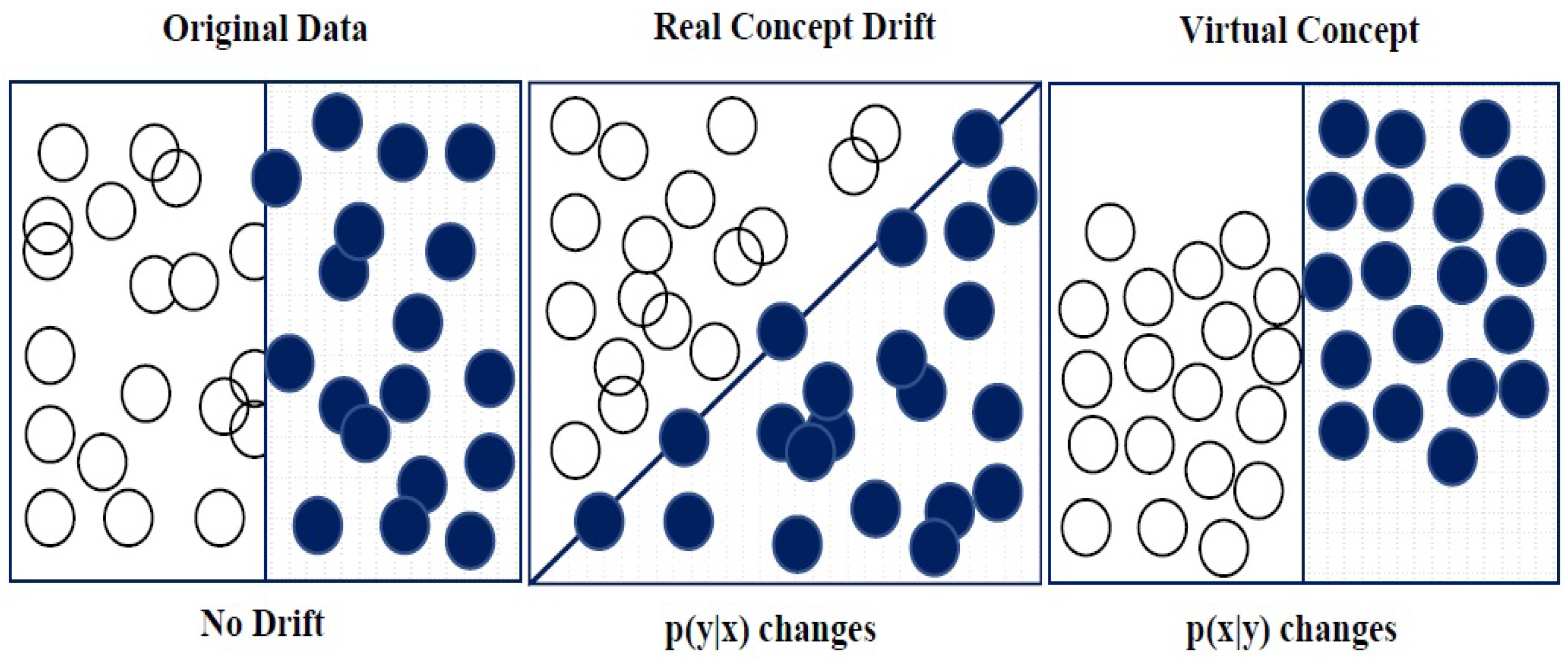
According to the Bayesian decision theory [9], a classification model can be described by the prior probabilities of classes p ( y ) and class conditional probabilities p ( x | y ) for all classes y∈ { K 1 , , K c }, where c is the number of predefined classes. A data point x i X has y j for all classes y { , 1 , , C } . If a data point x j X has y j = , then it is unlabelled. Therefore, the classification decision for instance X at equal costs of mistake is made based on maximal a posteriori probability, which for class y can be represented as p ( y | X ) = p ( y ) p ( X | y ) / p ( X ) where p ( X ) = y = 1 c p ( y ) p ( X | y ) .
In nonstationary environments, changes in a data stream are reflected by the probability distributions in an event called concept drift. Concept drift means that the concept about which the data are being collected may shift after some minimal stable period [8]. Formally, concept drift between time point t 0 and time point t 1 can be defined as follows.
Definition 1.
For a given data stream S, we say that concept drift occurs between two distinct points in time, t and t + Δ , i f   f     x :   p t ( x , y ) p t + Δ ( x , y ) where p t denotes the joint distribution at time t between the set of input attributes and the class label.
By considering this, any changes in incoming data can be characterized by changes in components of the Bayesian decision theory [10]:
  • Prior probabilities p ( y ) are prone to changes.
  • Probabilities p ( X | y ) of class conditional are also prone to changes.
  • Consequently, posterior probabilities p ( y | X ) may/may not change.
Based on the cause and effect of these changes, as shown in Figure 1, two types of drift are identified: real drift and virtual drift [8,11,12]. Real drift is defined as changes in p ( y | X ) . Note that such changes can occur with or without changes in p ( x ) ; thus, they may or may not be visible from the data distribution without knowing the true class labels. Virtual drift is defined as changes in the p ( x ) or class p ( y ) distributions that do not affect p ( y | X ) . As we are mostly interested in the effect of concept drift on classification, we focus on methods that use true class labels to detect drift. We, therefore, concentrate mainly on real drift, regardless of whether they are visible from the input data distribution p ( x ) .
Furthermore, in terms of class distribution, researchers differentiate how these changes happen, as shown in Figure 2. A sudden/abrupt drift happens when the source distribution in S t at a moment in time t is suddenly substituted by another distribution S t + 1 . Gradual drift is connected with a slower rate of change and it refers to a transition stage where examples of two different distributions P j and P j + 1 are mixed, whereas in recurring drift, after a period of time, previous concepts may reappear again. We emphasise that the proposed drift detector has been designed mainly for sudden/abrupt drift.

Existing Concept Drift Detection Methods

This section describes some well-known drift detectors that are related to our work:
DDM: Drift Detection Method. This method, developed in [13], is the most recognized work in this field. The method uses a classifier error that is normally reduced as more training examples are used. When an increase in the number of training examples also increases the classifier error, the model must be rebuilt. This indicates that sudden drift might have occurred. This model introduces a warning level when the error rates have increased to a certain level. Upon reaching the warning level, incoming new examples will be treated in a special window. If within this special window the error keeps increasing to a drift level, then the current classifier is rebuilt by learning from examples within the special window.
EDDM: This method, proposed by the authors of [14], is an adjustment of DDM. The same warning alarm mechanism that is used by DDM is used in EDDM, however; instead of monitoring error rate, EDDM monitors the distance between two sequential errors. Consequently, when the concepts of incoming data are stable, the distance between the two sequential errors decrease; otherwise, warnings and drifts are signalled.
FHDDM [15] is a method for detecting drifts using Hoeffding’s inequality through a window of size n. This window detects a drift if a considerable variation is observed between the current probabilities and the maximum of correct predictions. By using the error’s probability ( δ , default 10–7), FHDDM finds the variations among the probabilities ( Δ P ) and the threshold (∈). Consequently, FHDDM will signal a drift if Δ P .
PH Test: This method introduced in [16] is typically used for detecting drifts in applications of signal processing. In this work, between the observed values and their mean till current time T, a cumulative difference is represented as a variable m T . The variable of m T is calculated via m T = t = 1 T ( x t x T δ ) , where x T = 1 T t = 1 T x t and δ matches to the changes in magnitude that are allowed. The minimum m T which is denoted as M T , is also updated through M T   =   m i n ( m T , t = 1 T ) . Subsequently, a concept drift is signalled when there is a considerable variation between m T and M T i.e., P H T : m T M T > λ where λ is a user predefined threshold. However, increasing the value of λ causes fewer false alarms, but it increases the false negative rate.
SEED: This method, proposed in [17], within a window W, compares two sub-windows. The older part of this window is dropped when there is a distinct average exhibited by the two sub-windows. Hoeffding Inequality with Bonferroni correction is used by SEED to calculate its test statistic, performing block compression in order to remove unnecessary cut points and then blocks that are homogeneous in nature are merged.
STEPD: STEPD is a method proposed by [18] over two windows, namely, recent and older, which calculates statistical tests with continuity correction. Within a concept, the accuracy of the learner using the two windows is expected to be stable. When there is a significant difference in the accuracy of the recent window, warning and drift are signalled.
RDDM: This method, developed in [19], solves the problem of a performance losing of DDM, which is caused by decreasing sensitivity which requires many examples for drift detection. This method uses a mechanism to abandon older examples, regularly recalculating the statistics of RDDM which are responsible for detecting drifts. The authors found that RDDM delivers higher accuracy than DDM in most cases, by detecting drifts earlier, despite an increase in false positives and memory consumption.
DetectA: This method proposed in [20] is a proactive approach called Detect Abrupt Drift (DetectA) for sudden drift detection. Three steps are used to describe this method: (i) this method labels the patterns from the test set using an unsupervised method; (ii) from the training and test sets, some statistics will be computed, conditioned to the given class labels the training set; and (iii) a multivariate hypothesis test used to compare the training and testing statistics. Finally, based on this test, DetectA attempts to detect drift on the test set before the real labels are obtained.
NN-DVI: This method proposed by the authors of [21] uses a regional-density estimation as a drift detection method, named nearest neighbour-based density variation identification (NN-DVI). This method consists of three components: (i) k-nearest neighbour-based space-partitioning schema (NNPS), which transforms unmeasurable discrete data instances into a set of shared subspaces for density estimation; (ii) the density discrepancies are accumulated by a distance function in these subspaces and quantifies the overall differences; (iii) the statistical test defines the confidence interval to detect drift. Note that two windows of data are used by NN-DVI and these are compared to detect drift.
HLFR: This method by [22] uses Hierarchical Linear Four Rates. HLFR runs using two layers: the responsibility of detecting potential drifts belongs to the first layer, whereas the second layer validates the detected drift and communicates this information back to the first layer. Layer one observes the same four rates of the confusion matrix. Consequently, if a drift is detected, a permutation test is applied by layer two to confirm if the detected drift is true or false. However, if the drift is false, the testing process restarts.
FPDD, FSDD, and FTDD: These methods are proposed by [23]. Each of these methods uses a different statistical test and then measures the difference in errors rather than correct predictions. For example, when the number of errors or correct predictions is smaller than five, the Fisher’s Exact test will be used by FPDD. On the other hand, instead of using the test of equal proportions, the chi-square test for homogeneity of proportions is applied by FSDD.

3. The Proposed Approach

In nonstationary environments and in the presence of concept drift, existing drift detectors analyse the prediction results of the base learner and apply a certain decision model to signal a drift when changes are detected. Generally, most of the existing drift detectors, including the aforementioned methods, evaluate prediction results by analysing the error rate (accuracy) and its corresponding standard deviation, and find the difference between the means of the sub-windows or compare the accuracy of a model with different time windows, etc. [7]. This evaluation method is a measure of the classification performance to evaluate learning algorithms. Conversely, the drift detection method proposed in this paper for a nonstationary environment is quite different.
This paper proposes a data stream model that reacts quickly to sudden drift, consuming minimal time and memory compared to the state-of-the-art. In a novel way, we combine a diversity measure called a disagreement measure known from static learning in streaming scenarios with a modified PH test. Instead of monitoring the error estimates, DMDDM-S monitors the diversity of a pair of classifiers, where the true label of an example is not necessary to determine whether components disagree. In addition, we adopt k-prototype clustering as a solution to label the unlabelled data and use the newly labelled data with the labelled ones to retrain the model to be consistent with the current concept. In this paper, DMDDM-S is proposed to judge diversity based on an examination of classifier responses to changes in incoming data.

3.1. Pairwise Diversity Measures

Diversity is an important characteristic of ensembles in the standard, static data context. Measuring diversity can be useful to analyse the effectiveness of a diversity-inducing method. Therefore, many researchers consider diversity to prune a number of component classifiers [24,25], measure the diversity in decision forests [26] or characterize the diversity between classifiers [27].
In addition, there have been scant attempts at promoting diversity. For example, the authors of [28] discuss the impact of diversity on online ensemble learning and reactions to drift by modifying the Poisson distribution used in online bagging. However, by doing so, they only measure the accuracy of the modified ensemble, not its diversity. Recently, another work considers diversity [29] in an experiment using sliding windows. Therefore, to the best of our knowledge, our approach is the first semisupervised drift detection method to measure the diversity of component classifiers directly and use it as a base for drift detection. In contrast, the previous approaches used classification accuracy to detect drifts.
Informally, for a pair of classifiers in a binary classification problem, each component gives one of two possible predictions for each example, let us say 0 (negative class) or 1 (positive class). If we take the predictions of each component, we can calculate the disagreement between these predictions. Therefore, it is about the disagreement between the predictions of pairs of component classifiers, regardless of the true labels.
Formally, the diversity of component classifiers (e.g., disagreement) can be calculated in pairs, for example, let X = x 1 , , x n be a labelled data set and y v = [ y v ( x 1 ) , , y v ( x n ) ] an n-dimensional binary vector that represents the output of a classifier h v , such that y v ( x j ) = 1, if h v correctly predicts the class label, and 0 otherwise. Table 1 presents all the possible outcomes for a pair of classifiers h u and h v , such that h u = h v , where N a b is the number of instances x j X for which y u ( x j ) = a and y v ( x j ) = b . Therefore, all the probabilities of N a b are as follows.
  • N 10 number of examples where h u predicts class 1 and h v predicts class 0.
  • N 01 number of examples where h v predicts class 1 and h u predicts class 0.
  • N 11 number of examples where h u predicts class 1 and h v predicts class 1.
  • N 00 number of examples where h u predicts class 0 and h v predicts class 0.
Formally speaking, the disagreement measure is defined as the ratio of the number of inconsistent decisions over the total number of observations. Also, we can say it is the ratio between the number of observations for which one classifier is correct and the other is incorrect. Consequently, the diversity measure reflects the variety of responses of classifiers to changes of incoming data. The disagreement measure is probably the most intuitive measure of diversity between a pair of classifiers [30]. Thus, calculating the diversity between two base classifiers ( h u and h v ) using the disagreement measure is measured by Equation (1):
D u : v = N 10 + N 01
On the other hand, the PH test considers a variable m T which measures the accumulated differences between observed values e (error estimates). Two basic approaches to calculate these values prequentially are fading factors and sliding windows. Over time, the fading factors deduct outdated information via multiplying the former summary by a factor and then adding a new value calculated using the incoming data. Other approaches use the sliding windows to hold at each time point a set of d most current examples in order to limit the amount of analysed examples. According to the authors of [16], the fading factors approach uses less time and memory compared with the sliding windows approach. Therefore, the fading factors approach is the one that is used in this work.
Using the fading factor, we calculate the fading sum S x , α and fading increment N α at time t from a stream of objects x, as follows,
S x : α ( t ) = x t + α × S x : α ( t 1 )
N α ( t ) = 1 + α × N α ( t 1 )
where S x : α ( 1 ) / N α ( 1 ) = x 1 and α (0 ≪ α ⩽ 1 ) is a constant determining the forgetting factor of the sum, which should be close to 1 (for example 0.999). Then, the fading average is computed at observation i as
M α ( t ) = S x : α ( t ) N α ( t )
Consequently, in this work, we use the studied diversity measures as the observed value instead of the error rate. By applying the value of diversity from Equation (1) in Equation (2), we have the following equations.
S u : v : α ( t ) = D u : v + α × S u : v : α ( t 1 )
M α ( t ) = S u : v , α ( t ) N α ( t )
Equation (6) can be used with the PH test to monitor the diversity of a pair of classifiers. Then, Equation (7) is used to calculate the cumulative difference m T between the observed values and their mean till the current moment t where x T = 1 T t = 1 t x t and δ corresponds to the magnitude of changes that are allowed. The minimum value of this variable is also computed via Equation (8). As a final step, the test monitors the difference between M T and m T via Equation (9). When this difference is greater than a given threshold ( λ ), a drift is signalled.
m T = t = 1 T ( x t x T δ )
M T = m i n ( m t , t = 1 T ) .
P H T = m T M T

3.2. K-Prototype Clustering

To label the unlabelled data, it is worth mentioning some semisupervised learning methods. Some of these are appropriate for processing data streams incrementally, namely co-training, tri-training, self-training and K-prototype clustering. Considering incoming data have both numeric and categorical values, we propose to adopt K-prototype as a solution to our semisupervised drift detector, though a number of unlabelled data are extracted from the incoming data. Then, by applying K-prototype clustering to these data, we can get labels for all these unlabelled data.
The work in [31] proposes an algorithm based on the k-means paradigm but removes the numeric data limitation whilst preserving its efficiency. The K-prototype algorithm integrates the k-means and k-mode algorithms to deal with mixed data types. Therefore, the k-prototype algorithm is more useful practically because data collected in the real world are of mixed types. Assume a set of n objects, X = { X 1 , X 2 , , X n } ; X i = { X i 1 , X i 2 , , X i m } consists of m attributes. The goal of clustering is to partition n objects into k disjoint clusters C = { C 1 , C 2 , , C k } , where C i is an i-th cluster center. The distance d ( X i , C j ) between X i and C j can be calculated as follows,
d ( X i , C j ) = d r ( X i , C j ) + γ d c ( X i , C j )
where d r ( X i , C j ) is the distance between numerical attributes, d c ( X i , C j ) is the distance between categorical attributes, and γ is a weight for categorical attributes.
d r ( X i , C j ) = i = 1 p | x i l C j l | 2
d c ( X i , C j ) = i = p + 1 m δ ( x i l C j l )
In Equation (11), d r ( X i , C j ) is the squared Euclidean distance measure between cluster centres and an object on the numerical attributes; whereas, in Equation (12), d c ( X i , C j ) is the simple matching dissimilarity measure on the categorical attributes, where δ ( x i l C j l ) = 0 for x i l = C j l and δ ( x i l C j l ) = 1 for x i l C j l .

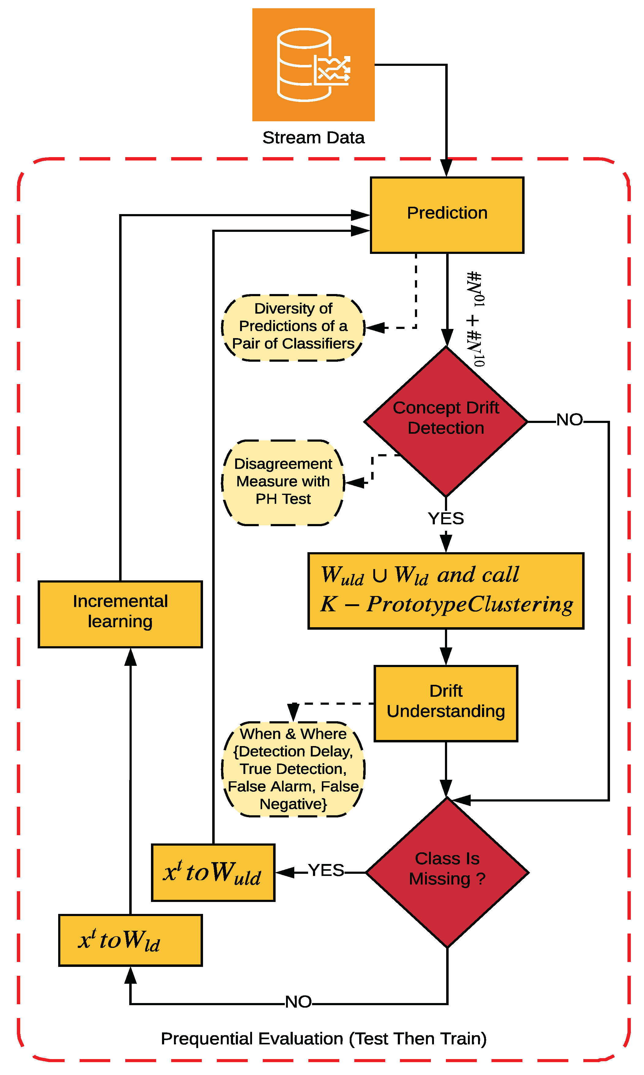
3.3. The DMDDM-S Algorithm

The DMDDM-S approach is presented in Algorithm 1 and its framework is shown in Figure 3. First, the algorithm processes each example from the data stream and obtains the predictions for a pair of classifiers on each example line (lines 1–3). Then, the algorithm builds the outputs, as shown in Table 1. As shown in Table 1, we need to find the two cases ( N 10 and N 01 ) where the pair of classifiers performs differently. Once we observe this disagreement, we count the number of observations on which one classifier is correct and the other is incorrect, shown in lines 4 to 9, respectively. These steps represent the first phase of the DMDDM-S framework (prediction phase).
Phase two (concept drift detection phase) uses these observed predictions using a disagreement measure with the PH test to detect drifts. In line 10, we apply the disagreement measure (Equation (1)) by aggregating these observations and dividing it by the number of component classifiers. Then, the fading factor approach is applied from lines 11 to 13 (Equation (5), Equation (3) and Equation (6)). In lines 11 and 12, the fading sum and fading increment are calculated, respectively. With the fading sum and fading increment, we use the value of diversity from line 10 as the observed value instead of the error estimates that were used in the original PH test. In line 13, the fading average is calculated. To monitor the diversity of a pair of classifiers from lines 14 to 19, the modified PH test considers a variable m T , which measures the accumulated difference between the observed value of diversity and their mean up to the current moment (Equation (7)). After each observation, the PH test checks whether the difference between the current m T and the smallest value up to this moment M T is greater than a given threshold (Equation (9)). If the difference exceeds the predefined threshold, a drift is signalled. When there is a drift, we need to label the current unlabelled data to use them to retrain the model and keep it consistent.
Therefore, line 20 combines the two windows of the labelled ( W l d ) and unlabelled data ( W u l d ) and sends the result to K-prototype clustering in order to label the unlabelled data in line 21, the third phase of the DMDDM-S framework. When there is a drift, phase four (drift understanding) starts, which evaluates the detected drift in terms of delay detection, true detection, false alarm and false negative. The evaluation method is explained in Figure 4.
Then, lines (22–24) incrementally train the current model and keep it up-to-date with the newly labelled data ( N l d ). Lines (26–39) check and handle the availability of each class, phase five (class is missing?). With each observation of x t and whether there is a drift or not, we need to check if x t is labelled or not. If the class of x t is missing, first line 27 checks if ( W u l d ) reached the pre-defined probability, removes the oldest instance in ( W u l d ) and adds the newest one to ( W u l d ); otherwise, x t is added to ( W u l d ) directly, line 30. On the other hand, if the class is not missing, line 33 will incrementally train the current model with the current labelled instance. Finally, lines (35–39) check the dynamic window of labelled data ( W l d ), If the size of this window reaches the pre-defined probability, we start removing the oldest one and add the newest labelled; otherwise, x t is added to ( W l d ).
Algorithm 1: Pseudocode of Diversity Measure as a Drift Detection Method in a Semi-Supervised Environment (DMDDM-S)
Applsci 10 00606 i001

4. Drift Detector Evaluation

The performance of DMDDM-S is evaluated against various drift detectors, namely, DDM, EDDM, FHDDM, PH Test, SEED, STEPD and RDDM. The main reasons for choosing these supervised methods over semisupervised methods are: (i) the limited access to the source code of some works, and (ii) we want to show the strengths of DMDDM-S, which can detect drifts faster when only 50% of the data is labelled with minimal consumption in terms of memory and run time than the existing methods that use 100% of labelled data.
Following the literature [13,14,15], we use the three synthetic datasets (https://github.com/alipsgh/data_streams) for the evaluation, namely Mixed, Sine1 and Sine2, with two classes and holding 100,000 instances. In addition, 10% of noise is added to each dataset. By doing this, we can determine how robust a drift detector is against a noisy data stream. Thus, the main advantage of using a synthetic dataset is that we are able to determine the true location of drifts in a data stream.
  • Mixed: This dataset has two numeric attributes, x and y, uniformly distributed in [0, 1] as well as two Boolean attributes v and w. The instances are classified as positive if at least two of the three following conditions are satisfied: v , w , y < 0.5 + 0.3 × sin ( 2 π x ) . The classification is reversed after drifts. Sudden drifts happen at every 20,000 instances.
  • Sine1: This comes with two attributes (x and y), which are uniformly distributed in [0, 1]. Following a function y = s i n ( x ) for classification, any instances below the curve are classified as positive, while the others are classified as negative, till the first drift occurs. At every 20,000 instances, a drift will occur and then the classification is reversed.
  • Sine2: This comes with two attributes (x and y) which are uniformly distributed in [0, 1]. Following a function 0.5 + 0.3 × sin ( 3 × π × x ) , instances under the curve are classified as positive while the other instances are classified as negative. At every 20,000 instances, a drift will occur and then the classification is reversed.
Furthermore, the proposed algorithm and the ones used for comparison are implemented in Java as part of the Massive Online Analysis (We had to remove the label from some training instances (50%) to simulate a semisupervised environment. Where a semisupervised setting assumes some input (training), the instances will not be labelled) (MOA) framework [32]. The experiments are conducted on a machine equipped with Intel Core i7 @ 3.4 GHz with 16GB of RAM running windows 10. To make the comparison more meaningful, we set the same parameter values for all the algorithms. For DMDDM-S, due to an experiment not mentioned in this work, we use the Hoeffding tree (HT) and Perceptron (PER) as our incremental classifiers. Because of their incremental nature, they are high-grade at describing changes over time. In addition, we use the PH test parameters ( λ = 100, δ = 0:1) as proposed in [16] and Forgetting factor ( α = 0.9996). For base classifier consistency, all the compared drift detectors are run using Hoeffding tree (HT) and Perceptron with the default parameters as set in MOA (or as in the original papers).
Regarding the evaluation process, recall the four requirements which need to be met by a model that operates in a nonstationary environment, hence we evaluate our detector and the competitors as shown in Figure 4. Figure 4 illustrates the DMDDM-S evaluation. The straight arrow represents the main stream of incoming data and the crosses show the real position of drifts. We calculate the delay of drift detection by defining a value Δ that represents the length of an acceptable drift delay. This value works as a threshold to locate the distance of the detected drift from the real position of the drift. Therefore, by considering this value Δ , we describe the following measures.
  • Detection Delay (Delay): The number of examples between the actual position of the drift and the detected one.
  • True Detection (TD): Detects a drift occurring at time t and within [ t + Δ ].
  • False Alarm: A detector falsely signals a drift outside [ t + Δ ].
The length of the acceptable drift delay Δ is set to 250 on the synthetic datasets as used in [15]. In addition to the above measures, the detection runtime (in milliseconds), memory usage (in bytes) and accuracy are also considered as shown below. Finally, in all the experiments, incoming data are processed prequentially, which means testing the instances first and then using them to train the model. In this direction, we run each detector 100 times and average the results.
  • Detection Runtime (Time): The time required to detect the drift.
  • Memory Usage: Memory requirement.
  • Accuracy: Accuracy of classifiers after the drift is detected (calculated by counting the number of correct predictions). This value is displayed by MOA.
  • MeanAccuracy: Mean accuracy over the data stream (also by MOA).

Experiment Results and Analysis

This section presents the results of the experiments and the analyses of each drift detector, where Table 2, Table 3 and Table 4 show the results of the experiments using Sine1, Sine2 and the Mixed datasets. The results of the Sine1 and Mixed datasets are similar. For example, the method that detects drift the fastest is STEPD, followed by our proposed method, DMDDM-S, and then FHDDM, SEED and RDDM in ascending order of delay detection. In addition, all methods detect all the drifts correctly. In relation to Sine2, DMDDM-S has the lowest average delay detection followed by STEPD, FHDDM, and SEED, respectively. In relation to computational time and memory usage, it is clearly seen that SEED, RDDM and FHDDM have the highest memory usage compared to the others. This is because these methods require more memory for storing the prediction results in the sliding windows or repositories and they use more computational time due to subwindow compression or reservoir sampling procedures. In addition to obtaining first and second place in delay detection, DMDDM-S has the lowest computational time and memory usage. The main reason for this is because DMDDM-S maintains a small number of variables compared with the others, which results in less memory usage and less execution runtime to update these variables.
Regarding false alarm, DMDDM-S has relatively high readings, due to the parameter sensitivity of DMDDM-S. For example, as shown in Figure 5a,c, increasing λ (100–200–300) will entail fewer false positives (as shown in Figure 5a) but might delay change or miss detection (as shown in Figure 5c), resulting in a trade-off between false positives and delay change detection.
Even with this increase, DMDDM-S is one of the highest in terms of delay detection and incurs the lowest time and memory consumption.
Furthermore, despite this trade-off, the accuracy of DMDDM-S is constant over the sensitivity of parameters, as shown in Figure 5e. As mentioned in [16], the trade-off exists with the use of the PH test; consequently, one possible solution to overcome this trade-off is to control the diversity of the disagreement method using two fading factors instead of one as used in this work. Such a solution is left for future work. Moreover, Figure 5b,d,f shows the stability of each detector in terms of accuracy and mean accuracy over the data stream, where DMDDM-S is among the highest and most stable compared to the others.

5. Conclusions

In this work, we introduced a new drift detector, called DMDDM-S, which adapts the disagreement measure and uses its calculations with the PH test to detect concept drift. DMDDM-S is proposed to calculate the diversity of classifier responses according to the evolving incoming data. Therefore, instead of monitoring the error estimates, DMDDM-S monitors the diversity of a pair of classifiers using the fading factor. In this way, the PH test is triggered whenever the predictions of components ( h u and h v ) start to disagree in an unusual way. The results of the experiments on the synthetic datasets indicate that with a lack of class labels, DMDDM-S detects drifts with shorter delay and with minimal detection runtime and memory usage compared to the existing methods. In the future, there is potential to improve DMDDM-S. DMDDM-S is designed for binary classification problems. For multiclass classification problems, the current method may fail to measure the differences between classifiers that incorrectly predict the same instance using different labels. Consequently, we plan to extend the proposed method using multiclass classification problems.

Author Contributions

Conceptualization, O.A.M. and E.P.; Methodology, O.A.M.; Software, O.A.M.; Validation, E.P., N.A. and E.P.; Formal analysis, O.A.M.; Investigation, O.A.M.; Data curation, O.A.M.; Writing—original draft preparation, O.A.M.; Writing—review and editing, E.P., J.C. and N.A.; Visualization, O.A.M.; Supervision, E.P. and J.C. All authors have read and agreed to the published version of the manuscript.

Funding

This research received no external funding.

Conflicts of Interest

The authors declare no conflicts of interest.

References

  1. Prasad, B.R.; Agarwal, S. Stream data mining: Platforms, algorithms, performance evaluators and research trends. Int. J. Database Theory Appl. 2016, 9, 201–218. [Google Scholar] [CrossRef]
  2. Haque, A.; Khan, L.; Baron, M.; Thuraisingham, B.; Aggarwal, C. Efficient handling of concept drift and concept evolution over stream data. In Proceedings of theIEEE 32nd International Conference On Data Engineering (ICDE), Helsinki, Finland, 16–20 May 2016; pp. 481–492. [Google Scholar]
  3. Chen, Y.; Li, O.; Sun, Y.; Li, F. Ensemble Classification of Data Streams Based on Attribute Reduction and a Sliding Window. Appl. Sci. 2018, 8, 620. [Google Scholar] [CrossRef] [Green Version]
  4. Khamassi, I.; Sayed-Mouchaweh, M.; Hammami, M.; Gh edira, K. Discussion and review on evolving data streams and concept drift adapting. Evol. Syst. 2018, 9, 1–23. [Google Scholar] [CrossRef]
  5. Alippi, C.; Qi, W.; Roveri, M. Learning in nonstationary environments: A hybrid approach. In Proceedings of the International Conference on Artificial Intelligence and Soft Computing, Zakopane, Poland, 11–15 June 2017; Springer: Cham, Switzerland, 2017; pp. 703–714. [Google Scholar]
  6. Ditzler, G.; Roveri, M.; Alippi, C.; Polikar, R. Learning in nonstationary environments: A survey. IEEE Comput. Intell. Mag. 2015, 10, 12–25. [Google Scholar] [CrossRef]
  7. Barros, R.S.M.; Santos, S.G.T.C. A large-scale comparison of concept drift detectors. Inf. Sci. 2018, 451, 348–370. [Google Scholar] [CrossRef]
  8. Gama, J.; Žliobaitė, I.; Bifet, A.; Pechenizkiy, M.; Bouchachia, A. A survey on concept drift adaptation. ACM Comput. Surv. 2014, 46, 44. [Google Scholar] [CrossRef]
  9. Duda, R.O.; Hart, P.E.; Stork, D.G. Pattern classification. Int. J. Comput. Intell. Appl. 2001, 1, 335–339. [Google Scholar]
  10. Gao, J.; Fan, W.; Han, J.; Yu, P.S. A general framework for mining concept-drifting data streams with skewed distributions. In Proceedings of the the 2007 SIAM International Conference on Data Mining SIAM (2007), Minneapolis, MN, USA, 26–28 April 2007; pp. 3–14. [Google Scholar]
  11. Pesaranghader, A.; Viktor, H.L.; Paquet, E. McDiarmid drift detection methods for evolving data streams. In Proceedings of the 2018 International Joint Conference on Neural Networks (IJCNN), Rio de Janeiro, Brazil, 8–13 July 2018; pp. 1–9. [Google Scholar]
  12. Brzezinski, D. Block-Based and Online Ensembles for Concept-Drifting Data Streams. Ph.D. Thesis, Poznan University of Technology, Poznań, Poland, 2015. [Google Scholar]
  13. Gama, J.; Medas, P.; Castillo, G.; Rodrigues, P. Learning with drift detection. In Proceedings of the Brazilian Symposium on Artificial Intelligence, São Luís, Brazil, 29 September–1 October 2004; pp. 286–295. [Google Scholar]
  14. Baena Garca, M.; del Campo Avila, J.; Fidalgo, R.; Bifet, A.; Gavalda, R.; Morales Bueno, R. Early drift detection method. In Proceedings of the Fourth International Workshop on Knowledge Discovery from Data Streams, Berlin, Germany, 18–22 September 2006; Volume 6, pp. 77–86. [Google Scholar]
  15. Pesaranghader, A.; Viktor, H.L. Fast hoeffding drift detection method for evolving data streams. In Proceedings of the Joint European Conference on Machine Learning and Knowledge Discovery in Databases, Riva del Garda, Italy, 19–23 September 2016; pp. 96–111. [Google Scholar]
  16. Gama, J.; Sebastiao, R.; Rodrigues, P.P. On evaluating stream learning algorithms. Mach. Learn. 2013, 90, 317–346. [Google Scholar] [CrossRef] [Green Version]
  17. Huang, D.T.J.; Koh, Y.S.; Dobbie, G.; Pears, R. Detecting volatility shift in data streams. In Proceedings of the 2014 IEEE International Conference on Data Mining, Shenzhen, China, 14–17 December 2014; pp. 863–868. [Google Scholar]
  18. Nishida, K.; Yamauchi, K. Detecting concept drift using statistical testing. In Proceedings of the International Conference on Discovery Science, Sendai, Japan, 1–4 October 2007; pp. 264–269. [Google Scholar]
  19. Barros, R.S.; Cabral, D.R.; Goncalves, P.M., Jr.; Santos, S.G. Rddm: Reactive drift detection method. Expert Syst. Appl. 2017, 90, 344–355. [Google Scholar] [CrossRef]
  20. Escovedo, T.; Koshiyama, A.; da Cruz, A.A.; Vellasco, M. DetectA: Abrupt concept drift detection in nonstationary environments. Appl. Soft Comput. 2018, 62, 119–133. [Google Scholar] [CrossRef]
  21. Liu, A.; Lu, J.; Liu, F.; Zhang, G. Accumulating regional density dissimilarity for concept drift detection in data streams. Pattern Recognit. 2018, 76, 256–272. [Google Scholar] [CrossRef] [Green Version]
  22. Yu, S.; Abraham, Z. Concept drift detection with hierarchical hypothesis testing. In Proceedings of the 2017 SIAM International Conference on Data Mining, Houston, TX, USA, 27–29 April 2017; pp. 768–776. [Google Scholar]
  23. de Lima Cabral, D.R.; de Barros, R.S.M. Concept drift detection based on Fisher’s Exact test. Inf. Sci. 2018, 442, 220–234. [Google Scholar] [CrossRef]
  24. Banfield, R.E.; Hall, L.O.; Bowyer, K.W.; Kegelmeyer, W.P. A new ensemble diversity measure applied to thinning ensembles. In Proceedings of the International Workshop on Multiple Classifier Systems, Guildford, UK, 11–13 June 2003; Springer: Berlin/Heidelberg, Germany, 2003; pp. 306–316. [Google Scholar]
  25. Giacinto, G.; Roli, F. An approach to the automatic design of multiple classifier systems. Pattern Recognit. Lett. 2001, 22, 25–33. [Google Scholar] [CrossRef]
  26. Ho, T.K. The random subspace method for constructing decision forests. IEEE Trans. Pattern Anal. Mach. Intell. 1998, 20, 832–844. [Google Scholar]
  27. Skalak, D.B. The sources of increased accuracy for two proposed boosting algorithms. In Proceedings of the American Association for Arti Intelligence, AAAI-96, Integrating Multiple Learned Models Workshop, Portland, OR, USA, 4–5 August 1996; pp. 120–125. [Google Scholar]
  28. Minku, L.L.; White, A.P.; Yao, X. The impact of diversity on online ensemble learning in the presence of concept drift. IEEE Trans. Knowl. Data Eng. 2009, 22, 730–742. [Google Scholar] [CrossRef]
  29. Brzezinski, D.; Stefanowski, J. Ensemble diversity in evolving data streams. In Proceedings of the International Conference on Discovery Science, Bari, Italy, 19–21 October 2016; Springer: Cham, Switzerland, 2016; pp. 229–244. [Google Scholar]
  30. Kuncheva, L.I. Combining Pattern Classifiers: Methods and Algorithms; Wiley Interscience: New York, NY, USA, 2004. [Google Scholar]
  31. Huang, Z. Clustering large data sets with mixed numeric and categorical values. In Proceedings of the First Pacifc Asia Conference on Knowledge Discovery and Data Mining, Singapore, 23–24 February 1997; pp. 21–34. [Google Scholar]
  32. Bifet, A.; Holmes, G.; Kirkby, R.; Pfahringer, B. MOA: Massive online analysis. J. Mach. Learn. Res. 2010, 11, 1601–1604. [Google Scholar]
Figure 1. Types of drifts: circles represent instances, different colors represent different classes.
Applsci 10 00606 g001
Figure 2. Concept Drift Patterns.
Applsci 10 00606 g002
Figure 3. Framework of DMDDM-S.
Applsci 10 00606 g003
Figure 4. Illustration of the DMDDM-S evaluation.
Applsci 10 00606 g004
Figure 5. Changing DMDDM-S threshold (a,c,e) and the stability of each detector’s accuracy (b,d,f).
Applsci 10 00606 g005
Table 1. The correlation of a pair of classifiers (2 × 2).
h u = h v h u c o r r e c t ( 1 ) h u i n c o r r e c t ( 0 )
h v c o r r e c t ( 1 ) N 11 N 10
h v i n c o r r e c t ( 0 ) N 01 N 00
Table 2. Results of Sine1 dataset with (10% noise).
Sine1 (A)Sine1 (B)
Classifier Detector Delay TP Time Memory MeanAccuracy
HT & PreDMDDM-S36.37541.616886.631
HTFHDDM47.37547.7104885.242
DDM196.22523.347266.633
PHTest238.2751.22.1124066.211
STEPD27.0546.493687.047
SEED58.44123572.58886.969
RDDM9342.6865686.894
EDDM244.5250.11.614483.34
PreFHDDM46.56247.75104887.177
DDM154.63642.54547286.870
PHTest249.5680.0901.363124072.199
STEPD27.3545.293687.199
SEED56.8411.53593.60887.098
RDDM99.87542.6865687.075
EDDM25001.614472.181
Table 3. Results of Sine2 dataset with (10% noise).
Sine2 (A)Sine2 (B)
Classifier Detector Delay TP Time Memory MeanAccuracy
HT & PreDMDDM-S23.7541.716878.294
HTFHDDM52.12549.2104879.834
DDM209.23.61.547277.399
PHTest23001.9124057.738
STEPD33.146.493679.855
SEED62.4411.43638.35479.729
RDDM134.57543.8865679.55
EDDM2500214457.738
PreFHDDM56.675410.5104874.843
DDM246.250.32.147274.269
PHTest25001124049.882
STEPD41.72546.593674.851
SEED70.4410.63688.57674.813
RDDM189.6253.42865674.623
EDDM25001.414474.256
Table 4. Results of Mixed dataset with (10% noise).
Mixed (A)Mixed (B)
Classifier Detector Delay TP Time Memory MeanAccuracy
HT & PreDMDDM-S36.4541.216883.171
HTFHDDM48.149104872.767
DDM214.5751.81.942769.828
PHTest236.0251.31.6124067.876
STEPD28.747.693683.373
SEED60411.13609.60683.294
RDDM100.12543.4865683.265
EDDM25002.114457.858
PreFHDDM47.4547.6104882.125
DDM220.9252.11.942779.316
PHTest246.550.21.4124076.743
STEPD30.7254793682.143
SEED604113641.58982.065
RDDM117.57542.5865682.006
EDDM244.650.11.514476.483

