Article

Development of Stochastic Fatigue Model of Reinforcement for Reliability of Concrete Structures

1
Department of Civil Engineering, Aalborg University, 9100 Aalborg, Denmark
2
Department of Mechanical Engineering, Technical University of Denmark, 2800 Lyngby, Denmark
*
Author to whom correspondence should be addressed.
Appl. Sci. 2020, 10(2), 604; https://doi.org/10.3390/app10020604
Submission received: 15 November 2019 / Revised: 6 January 2020 / Accepted: 8 January 2020 / Published: 14 January 2020
(This article belongs to the Section Civil Engineering)

Abstract

:
This paper presents recent contributions to the Marie Skłodowska-Curie Innovative Training Network titled INFRASTAR (Innovation and Networking for Fatigue and Reliability Analysis of Structures-Training for Assessment of Risk) in the field of reliability approaches for decision-making for wind turbines and bridges . Stochastic modeling of uncertainties for fatigue strength parameters is an important step as a basis for reliability analyses. In this paper, the Maximum Likelihood Method (MLM) is used for fitting the statistical parameters in a regression model for the fatigue strength of reinforcement bars. Furthermore, application of the Bootstrapping method is investigated. The results indicate that the latter methodology does not work well in the considered case study because of run-out tests within the test data. Moreover, the use of the Bayesian inference with the Markov Chain Monto Carlo approach is studied. These results indicate that a reduction in the statistical uncertainty can be obtained, and thus, better parameter estimates are obtained. The results are used for stochastic modelling in reliability assessment of a case study with a composite bridge. The reduction in statistical uncertainty shows high impact on the fatigue reliability in a case study on the Swiss viaduct Crêt De l’Anneau.

1. Introduction

This paper presents statistical analyses performed on fatigue data obtained from [1], where laboratory fatigue tests were performed on reinforcement bars (rebars).
General methods and techniques utilized for risk and reliability assessment of civil engineering structures are presented [2,3,4,5,6,7,8,9,10,11,12,13,14,15,16,17,18].
Statistical analyses of the data are an essential step for the stochastic modeling of the material fatigue uncertainties, which can next be used as a basis for a probabilistic modeling and reliability analysis [19] of structures with reinforced concrete components, such as wind turbines and bridges [20,21]. Usually, foundations for onshore wind turbines are constructed by the use of reinforced concrete, which is also used in many bridges. Therefore, the development of stochastic models for the fatigue limit state and estimation of the resulting reliability can be considered as a contribution to reliability assessment of these types of structures, with respect to fatigue failure and also as the basis for the development of optimal strategies for the maintenance of wind turbines and bridges. [22].
Several methodologies can be used to estimate the statistical parameters. For instance: Maximum Likelihood Method (MLM), moment method, least square method, and Bayesian statistics. In the literature, there are some recommendations indicating which of these methods could be more suitable. At the same time, there is no unique answer to this question, especially for a fatigue case study on rebars. On the reliability assessment, choosing a specific method has a direct influence. In the reliability assessment, there is a need to have stochastic modeling for the material-resistance as well as for the loads. In this paper, the material-resistance model is presented in detail, and at the end, using a generic stochastic model for the fatigue load reliability results of a composite bridge are presented.
The MLM is chosen in this study as it gives an estimate of the statistical uncertainties [23]. MLM is considered for fitting the statistical parameters [2] in a regression model for fatigue strength. Typically, the statistical analyses are based on a limited number of data, for which MLM can provide estimates of the uncertainties associated with each of these parameters and the correlation between the parameters [24]. This paper also presents the use of the Bootstrap method, which generates synthetic data based on the available measurements from the experiment.
Further, Bayesian statistics is considered taking subjective/prior information into account. This is done with application of Bayesian inference with a Markov Chain Monte Carlo implementation [25,26,27]. Bayesian updating is an appropriate tool to update the structural performance function for fatigue by applying the information from the structural health monitoring and the prior information about different fatigue parameters. The aim is to compare the results of different methodologies and to provide information in order to select an appropriate method.
To study the effect of uncertainty of fatigue resistance model on the fatigue reliability of a structure, a case study of Swiss viaduct Crêt De l’Anneau is presented. For this structure, long term strain monitoring data on critical reinforcement is available.

2. Materials and Methods

2.1. Test Data

Test data on the fatigue strength test for steel reinforcement from the lab tests were done at Aalborg University by Hansen and Heshe [1]. It is utilized for the statistical analysis to determine typical fatigue strength uncertainties (see Table 1, where 1 indicated run-out/no failure and 0 indicates failure). The lab tests are performed with steel reinforcement bars with 16 mm of diameter and yields strengths of 570 MPa. The S-N curve for this data is presented in Figure 1. Run-outs are depicted in orange and failures in gray.

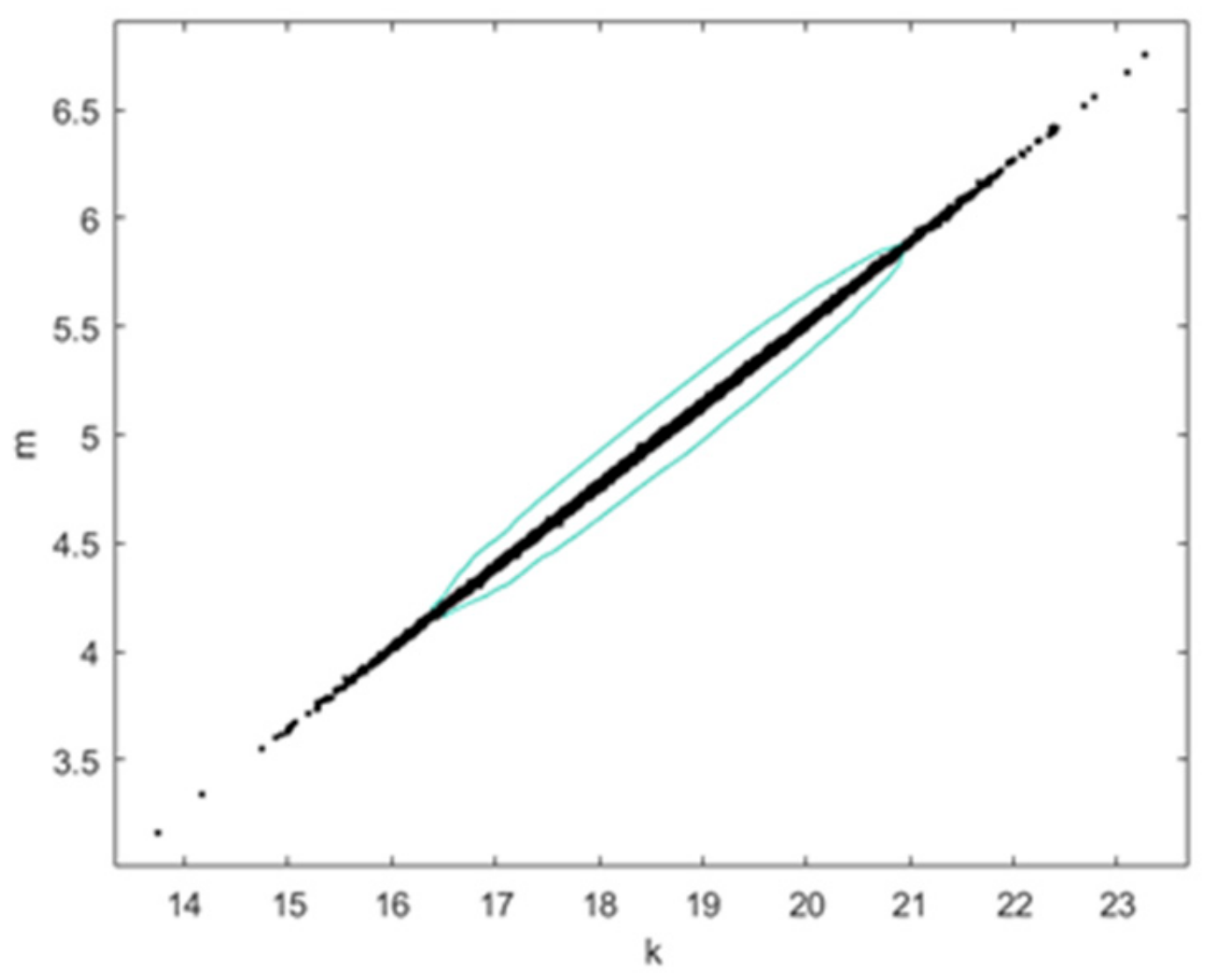
2.2. Statistical Analysis of Fatigue Data of Steel Reinforcing Bars

For steel reinforcement bars used in concrete S-N, curves are recommended by various international codes (such as Model code 2010, Model code 1990, DNV OS C 502, EN 1992-1) [28,29,30,31] and are generally written as:
n i = K   Δ s i m ,
or
log ( n i ) = log ( K ) m   log ( Δ s i ) ,
where n i is the number of cycles to failure with stress range   Δ s i in test number, i . K and m are fatigue parameters to be fitted by MLM here using test data [31].
To account for uncertainties in fatigue life, Equation (2) can be rewritten [22]:
log ( n i ) = log ( K ) m   log ( Δ s i ) + ε ,
where ε represents the uncertainty of the fatigue life model and is modelled by a stochastic variable with mean value equal to zero and standard deviation, σ ε . ε is often assumed to have a Normal distributed [31].
The Likelihood function to be used to estimate the optimal values of the parameters K , m , and σ ε from test data is written [22]:
L ( K ,   m , σ ε ) =   i = 1 n F P [ log ( K ) m   log ( Δ s i ) + ε = log ( n i ) ] × i = n F + 1 n F + n R P [ log ( K ) m   log ( Δ s i ) + ε > log ( n i ) ] .
Here, n i is the number of stress cycles to failure or to run-out with stress range Δ s i in test number i. n F is the number of tests where failure occurs, and n R is the number of tests where failure did not occur after n i stress cycles (run-outs). The total number of tests is n = n F + n R . K , m , and σ ε are obtained from the optimization problem m a x K , m , σ ε L K , m , σ ε , which can be solved using a non-linear optimization algorithm [31].
Run-outs contain information which from a statistical point of view has to be included in the statistical modelling in order to be consistent with all tests performed. This paper describes how run-outs can be included using the MLM. The number of cycles where the tests are stopped are often chosen in order to limit the costs and time used for the test campaign.
The terms in Equation (4) can be obtained from Equation (5) [22]:
P [ log ( K ) mlog ( Δ s i ) + ε = log ( n i ) ] = 1 2 π σ ε exp ( 1 2 ( log ( K ) m l o g ( Δ s i ) log ( n i ) σ ε ) 2 ) , P [ log ( K ) mlog ( Δ s i ) + ε > log ( n i ) ] = Φ ( log ( K ) mlog ( Δ s i ) log ( n i ) σ ε ) .
The parameters K , m , and σ ε are generally determined using a limited number of data. Consequently, the estimates are subject to statistical/parameter uncertainty. Since the parameters are estimated by the MLM, they become asymptotically (number of data should be >25–30). Normal distributed stochastic variables with expected values equal to the maximum-likelihood estimator and a covariance matrix equal to [32]:
C K , m , σ ε = [ H K , m , σ ε ] 1 = [ σ K 2 ρ K , m σ K σ m ρ K , σ ε σ K σ σ ε ρ K , m σ K σ m σ m 2 ρ m , σ ε σ m σ σ ε ρ K , σ ε σ K σ σ ε ρ m , σ ε σ m σ σ ε σ σ ε 2 ] .
  H K , m , σ ε   is the Hessian matrix with second-order derivatives of the log-likelihood function. σ K , σ m , and σ σ ε     denote the standard deviations of K , m , and σ ε , respectively, and e.g., ρ K , m is the correlation coefficient between K and m .

2.3. Bootstrap Method

The Bootstrap method developed by Efron [33] may be used for smaller samples and is quite flexible concerning the assumptions made. The Bootstrap method applies the actual distribution of the measurement errors, which are then propagated using an appropriate Monte Carlo scheme. That is, the Bootstrap method can be used to estimate the statistical (parameter) uncertainty.
Fatigue tests take very long time as it can take millions of cycles before the failure of one specimen, and changing the frequency of load application could lead to erroneous results. The Bootstrap method can be used to generate more synthetic data, which can then be used to estimate the parameter uncertainties as an alternative to the use of MLM described above.
Residuals are estimated by subtracting the calculated number of cycles to failure from the observed number of cycles in logarithmic scale. These residuals are plotted in Figure 2a, considering the case when run-outs are not included. This histogram indicates that an assumption of residuals as white noise is satisfactory and it is uniformly distributed with a mean value equal to zero. In this case, the Bootstrap method can be used, but in applications where run-outs are part of the data, the Bootstrap method cannot be used directly, as seen in Figure 2b.
If we plot the residuals along with their index (data number), they are random without considering run-outs, which is a basic requirement for using the Bootstrap method, as seen in Figure 3a. Random in this context means that residuals should not follow a pattern [34]. Whereas in Figure 3b with run-outs, residuals are following a pattern, so this requirement to apply the Bootstrap method is not fulfilled here.
Therefore, it can be concluded that Bootstrapping can be used for estimating parameter uncertainty only in the case of no run-outs.

2.4. Bayesian Inference with Markov Chain Monte Carlo Implementation

Bays’ rule provides the mathematical basis to update beliefs (prior information) about a variable, θ , given observations, y . By Bays’ rule, the posterior probability of θ given observations, p θ | y is obtained as follows [35,36]:
p θ | y = p θ p y | θ p y ,
Future predictions for y   * given observations y is obtained from the predictive distribution
p y * | y = p y * | θ p θ | y d θ ,
Thus, future predictions are modeled using the updated probability density function p θ | y similar to making a prediction for y   * using a single value of θ     in the classical statistical sense. Equation (8) can be estimated using Monte Carlo simulation strategies such as the Markov-Chain Monte-Carlo algorithm [36].
By definition, a Markov chain simulation is a sequence of random variables θ 1 ,   θ 2 ,   θ 3 ,       for which for any k , the distribution of θ   k depends only on the most recent one θ k 1 . In practice, several independent sequences of Markov chain simulations are created. The Metropolis algorithm is used to obtain the transition distribution function [31]. It is an adaption of a random walk that uses an acceptance/rejection rule to converge to the specified target distribution. The step-by-step procedure is as follows [27]:
  • Select initial parameter vector
  • Iterate as follows for k = 1 ,   2 ,   3 ,      
    a.
    Create a new trial position θ * = θ k 1 + Δ θ , where Δ θ is randomly sampled from the jumping distribution q Δ θ .
    b.
    Create the Metropolis ratio.
r = π θ * | y π θ k 1 | y ,
3.
Accept a new sample if:
θ k = θ *                   w i t h   p r o b a b i l i t y     m i n r , 1 θ k 1                                                                           o t h e r w i s e ,
Note that this requires the jumping distribution to be symmetric: q   θ * , θ k 1 = q   θ k 1 , θ * . If the jumping distribution is not symmetric, then the Metropolis-Hasting algorithm [37] can be used where both sides jumping distributions are part of the ratio.
Since the posterior distribution can be calculated by Equation (7), where p y is a normalizing constant, it also follows that the posterior density function can be written as:
p θ | y p θ p y | θ ,
i.e., the posterior distribution is proportional to the product of the prior and the likelihood functions.
If it is assumed that the prior distribution is the multivariate Normal distribution, then the Likelihood function becomes:
p y | θ , σ 2 = 1 σ 2 π e x p 1 2 σ 2 S S θ ,
where,
S S θ = i n y f S , θ 2 ,
The Metropolis ratio becomes:
r = p θ * | y , σ 2 p θ k 1 | y , σ 2 = e x p 1 2 σ 2 S S θ * S S θ k 1 ,
The scale reduction factor R indicates a potential scale reduction for the considered distribution when the number of samples goes to infinity (see [38] for theory and more detailed descriptions). The sampling is said to converge if R is close to one. Therefore, the number of simulations should be chosen such that R becomes as close to one as possible, and thereby, the Monte Carlo sampling error close to zero.
The parameters fitted in the SN-curve in Equation (1) are K and m . The correlation between them is illustrated in Figure 4. Here, the Markov Chain Monte Carlo algorithm is used. Furthermore, the Metropolis algorithm is applied for obtaining the transition distribution. Based on Reference [36], the scale reduction factor R is also calculated to 1.0007.

3. Results of Uncertainty Modelling

Table 2 shows a comparison between the results obtained by the methods presented above. This includes results obtained for the statistical parameters by MLM accounting for run-outs. Furthermore, a characteristic, 5% quantile is estimated using the MLM estimates resulting in log k   =   18.77 , which is larger than the characteristic value equal to 17.054 specified in the Eurocodes (see [38,39], and Table 2).
The Markov Chain Monte Carlo simulation results in Figure 5a show that log   k is mostly in the interval 18–19, and in Figure 5b, m is close to 5, which is in agreement with the fixed value used for MLM. It should be noted that m is assumed fixed in the reliability section. The Posterior marginal density function is also shown in Figure 6.

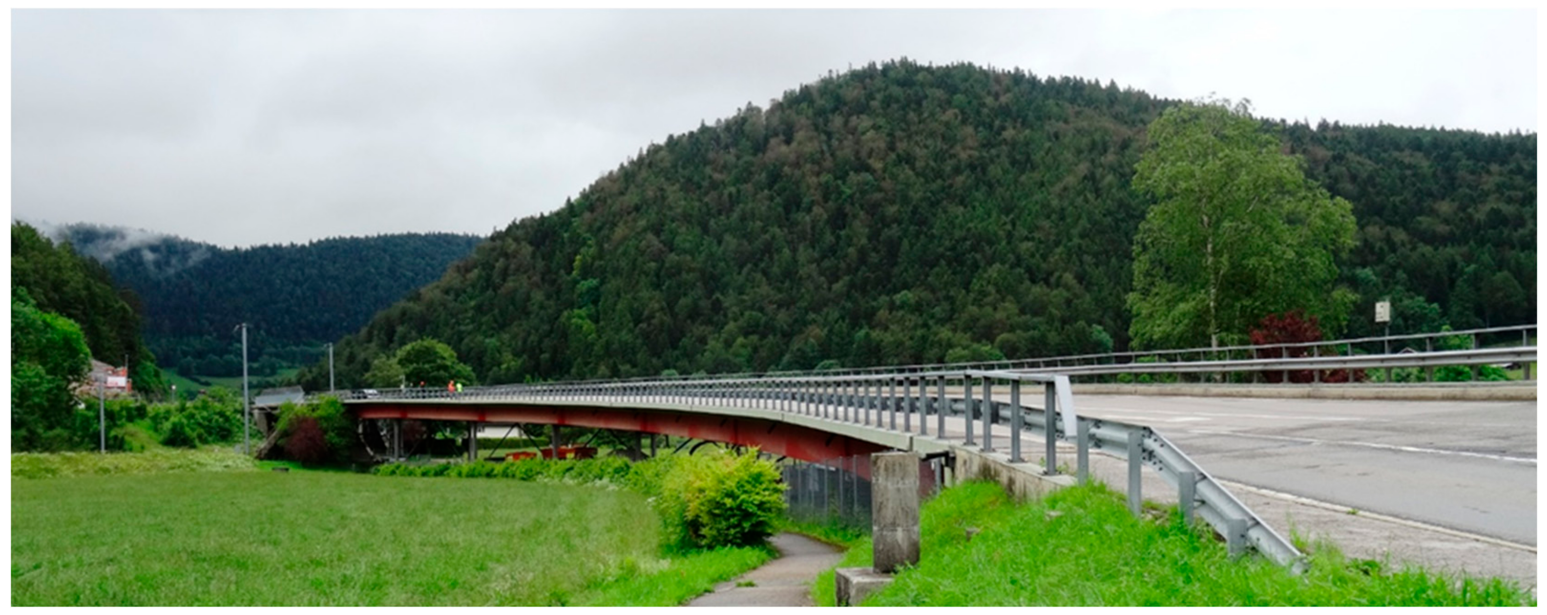
4. Case Study: Crêt De l’Anneau Viaduct

To illustrate the effect of change of model uncertainty of   log k , i.e., σ ε on the fatigue reliability of a structure, a case study of a composite (reinforced concrete deck and steel box girders) viaduct in Switzerland is chosen as seen in Figure 7.
The identified fatigue critical location of this composite bridge is the reinforced concrete slab, as shown in [40] p.41. The fatigue behavior of the reinforced concrete deck slab is mainly governed by transverse bending between two girders. It contributes also to local longitudinal bending under vehicle rolling wheel loads, thus it is double bending behavior. The MCS department at EPFL has installed electrical strain gauges on reinforcement bars at critical location. This monitored strain data is used as action effects to perform fatigue reliability analysis of the viaduct, a reliability framework presented in [41] is used for the purpose.

4.1. Limit State Equation

A limit state equation for fatigue failure of critical reinforcement in the viaduct is formulated based on the Palmgren-Miner rule [42,43] assuming linear damage accumulation, Equation (15), and [41,44].
g ( t ) = Δ i = 1 j X n n i t 10 ε · k ( X W R D Δ s i ) m = 0 ,
where
  • t indicates time 0 < t < TL in years,
  • T L is the service life time of the structure,
  • R D is modelling the ratio of design parameters, here the section modulus of the deck slab,
  • Δ s i   is the stress range for the ith load bin.
All other terms in the limit state equation are explained in Table 3.

4.2. Reliability Analysis

The First Order Reliability Method (FORM) is used for reliability analysis [2,46]. An open-source MATLAB-based toolbox, namely the FERUM (Finite Element Reliability Using MATLAB), is used for performing all FORM calculations [47]. The cumulative (accumulated) probability of failure in time interval [0, t] is obtained by Equation (16):
P F t = P g t 0 ,
The probability of failure is estimated by FORM [47]. The corresponding reliability index β t is obtained by Equation (17):
β t = ϕ 1 P F t ,
where, ϕ ( ) is standardized normal distribution function.
The annual probability of failure is obtained by:
Δ P F t = P F t P F t Δ t , t > 1 y e a r ,
where Δ t   = one year. The corresponding annual reliability index is denoted   Δ β .

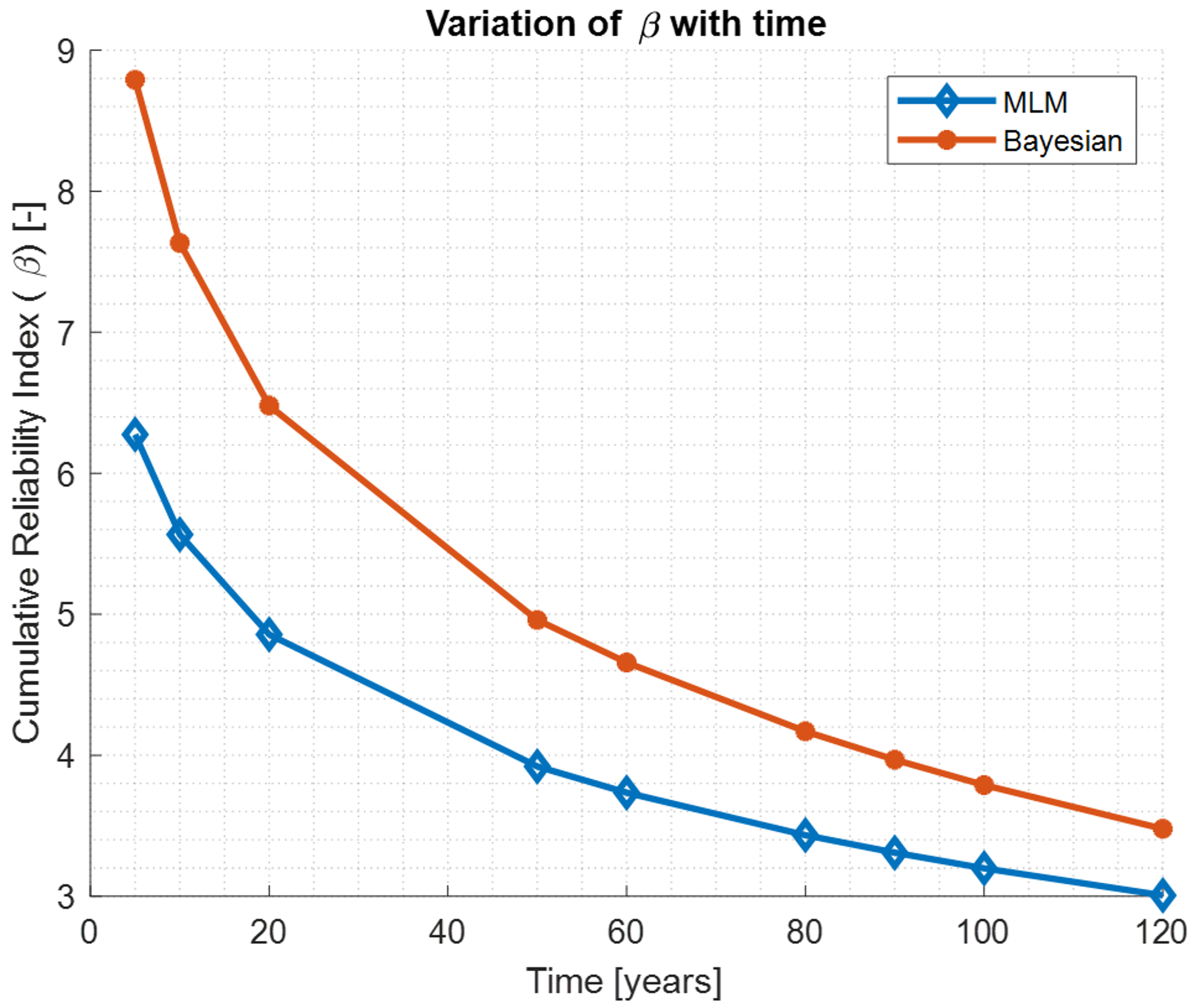
4.3. Reliability Results

The cumulative reliability index along the service life of the structure is presented in Figure 8 for the case where uncertainty in vehicle number X n is 1% and CoV for log K is as 0.39 (MLM) and 0.2 (Bayesian).
Corresponding annual reliability index at 120 years is presented in Table 4.
The actual stress in slab of viaduct is very low, thus exhibiting a very high fatigue reliability. Current results are shown for the case of scaled stresses. Even after the scaling of the stresses annual reliability index is within acceptable levels, which is more than 3.7 (for the case of very high consequence and low efficiency of intervention, [48]). Furthermore, it can be seen from the results that CoV for l o g K has a very high influence on reliability index. Thus, estimating the CoV with great accuracy is very important in order to estimate the safety of the structures reasonably.

5. Conclusions

In this paper, for stochastic modeling of uncertainties for fatigue strength parameter, MLM as a common methodology is utilized to fit the statistical parameters in a regression model based on available test data. The Bootstrapping method is used to generate synthetic data. Example investigations in this paper indicate that Bootstrapping cannot be used if run-out data are to be accounted for. Thus, further steps are not proceeded to estimate statistical parameters. It should be mentioned that if the Bootstrapping method was fulfilled the requirement (random pattern), another methodology such as least square method or even Bootstrapping could be used for parameter estimation in the next step. Subsequently, the use of Bayesian inference with the Markov Chain Monto Carlo approach is studied.
Reliability analysis of a selected detail in the Cret De l’Anneau Viaduct is used to illustrate and compare different stochastic models obtained by the statistical methods. The results obtained by MLM is used in reliability analyses and is assumed as a prior for Bayesian. The results show difference in the reliability indices, indicating the importance of accurate estimation of the model uncertainty of the SN-curve. The results emphasize the choice of statistical method as it influences the reliability analyses. In this case study, Bayesian provided better statistical uncertainty, hence better fatigue reliability assessment.

Author Contributions

The main idea for the paper was proposed by S.R. S.R. wrote the first draft of the paper, except Section 4 which was drafted by A.M. S.R., A.M. and S.B. provided literature review. S.R. developed the methodology wrote relevant codes for Maximum likelihood method, Markov Chain Monte Carlo, Bayesian inference and Bootstrap and reviewed by A.M. A.M. developed the reliability framework with relevant codes with input for stochastic model from S.R. S.R. and A.M. post-processed the results. J.D.S. supervised the findings of this work and reviewed methodology. S.R., A.M., J.D.S. and S.B. contributed for articulate the research work in its current form as full research manuscript. All authors discussed the results and contributed to the final results. All authors have read and agreed to the published version of the manuscript.

Funding

Current work is carried out under the project INFRASTAR (infrastar.eu), which has received funding from the European Union’s Horizon 2020 research and innovation program under the Marie Skłodowska-Curie grant agreement No. 676139. The grant is gratefully acknowledged.

Acknowledgments

These current codes were further developed based on codes provided in DTU Summer School on Uncertainty and sensitivity analysis of numerical models—7–11 August 2017, lecturer: Gurkan Sin, to suit current application.

Conflicts of Interest

The authors declare no conflict of interest.

References

  1. Hansen, L.P.; Heshe, G. Static, Fire and Fatigue Tests of Ultra High-Strength Fibre Reinforced Concrete and Ribbed Bars. J. Nord. Concr. Res. 2001, 26, 17–37. [Google Scholar]
  2. Sørensen, J. Notes in Structural Reliability Theory and Risk Analysis; Aalborg University: Aalborg, Denmark, 2011. [Google Scholar]
  3. Madsen, H.O.; Krenk, S.; Lind, N.C. Methods of Structural Safety; Prentice-Hall: Upper Saddle River, NJ, USA, 1986. [Google Scholar]
  4. Ditlevsen, O.; Madsen, H. Structural Reliability Methods; Wiley: Hoboken, NJ, USA, 1996. [Google Scholar]
  5. Faber, M.H. Risk Assessment in Engineering (Principles, System Representation & Risk Criteria). Available online: https://www.jcss.byg.dtu.dk/-/media/Subsites/jcss/english/publications/risk_assessment_in_engineering/jcss_riskassessment.ashx?la=da&hash=F4BD53E6E9C2AD6242FD54762719D55BD251A995 (accessed on 15 November 2019).
  6. Kaplan, S.; Garrick, B.J. On the Quantitative Definition of Risk. Risk Anal. 1981, 1, 11–27. [Google Scholar] [CrossRef]
  7. Modarres, M. Risk Analysis in Engineering: Techniques, Tools, and Trends; CRC Press: Boca Raton, FL, USA, 2006. [Google Scholar]
  8. Zio, E.; Baraldi, P.; Cadini, F. Basics of Reliability and Risk Analysis: Worked Out Problems and Solutions; World Scientific Publishing Co. Pte. Ltd.: Singapore, 2011. [Google Scholar]
  9. Zio, E. Introduction To The Basics Of Reliability And Risk Analysis [Elektronisk resurs]; World Scientific Publishing Co. Pte. Ltd.: Singapore, 2007. [Google Scholar]
  10. Chemweno, P.; Pintelon, L.; Muchiri, P.N.; Van Horenbeek, A. Risk assessment methodologies in maintenance decision making: A review of dependability modelling approaches. Reliab. Eng. Syst. Saf. 2018, 173, 64–77. [Google Scholar] [CrossRef]
  11. Aven, T.; Zio, E. Knowledge in Risk Assessment and Management; John Wiley & Sons: Hoboken, NJ, USA, 2018. [Google Scholar]
  12. Pham, H. Bayesian Inference for Probabilistic Risk Assessment; Springer: Berlin, Germany, 2005. [Google Scholar]
  13. Fenton, N.; Neil, M. Risk Assessment and Decision Anlysis with Bayesian Networks; CRC Press: Boca Raton, FL, USA, 2013. [Google Scholar]
  14. Singpurwla, N.D. Reliability and Risk. A Bayesian Perspective; John Wiley & Sons, Ltd.: Chichester, UK, 2006. [Google Scholar]
  15. Aven, T. Risk assessment and risk management: Review of recent advances on their foundation. Eur. J. Oper. Res. 2016, 253, 1–13. [Google Scholar] [CrossRef] [Green Version]
  16. Lair, J.; Rissanen, T.; Sarja, A. Methods for Optimisation and Decision Making in Lifetime Management of Structures. 2004. Available online: https://www.scribd.com/document/342349363/METHODS-FOR-OPTIMISATION-AND-DECISION-MAKING-IN-LIFETIME-MANAGEMENT-OF-STRUCTURES (accessed on 15 November 2019).
  17. Vrouwenvelder, A.; Holicky, B.M.; Tanner, C.P.; Lovegrove, D.R.; Canisius, E.G. Risk Assessment and Risk Communication in Civil Engineering. 2001. Available online: https://www.irbnet.de/daten/iconda/CIB14314.pdf (accessed on 15 November 2019).
  18. Bhattacharya, B. Risk and Reliability in Bridges. Innovative Bridge Design Handbook; Elsevier: Amsterdam, The Netherlands, 2016. [Google Scholar]
  19. Bahrebar, S.; Zhou, D.; Rastayesh, S.; Wang, H.; Blaabjerg, F. Reliability assessment of power conditioner considering maintenance in a PEM fuel cell system. Microelectron. Reliab. J. 2018, 88-90, 1177–1182. [Google Scholar] [CrossRef]
  20. Rastayesh, S.; Bahrebar, S.; Bahman, A.S.; Dalsgaard Sørensen, J.; Blaabjerg, F. Lifetime Estimation and Failure Risk Analysis in a Power Stage Used in Wind-Fuel Cell Hybrid Energy Systems. Electronics 2019, 8, 1412. [Google Scholar] [CrossRef] [Green Version]
  21. Rastayesh, S.; Long, L.; Dalsgaard Sørensen, J.; Thöns, S. Risk Assessment and Value of Action Analysis for Icing Conditions of Wind Turbines Close to Highways. Energies 2019, 12, 2653. [Google Scholar] [CrossRef] [Green Version]
  22. Màrquez-Dominguez, S. Reliability-Based Design and Planning of Inspection and Monitoring of OffshoreWind Turbines; Aalborg University: Aalborg, Denmark, 2013. [Google Scholar]
  23. Mankar, A.; Rastayesh, S.; Dalsgaard Sørensen, J. Sensitivity and Identifiability Study for Uncertainty Analysis of Material Model for Concrete Fatigue. In Proceedings of the 5th International Reliability and Safety Engineering Conference, Shiraz, Iran, 9–10 May 2018. [Google Scholar]
  24. Seber, G.; Wild, C. Non-Linear Regression; Wiley: Hoboken, NJ, USA, 1989. [Google Scholar]
  25. Rastayesh, S.; Bahrebar, S.; Blaabjerg, F.; Zhou, D.; Wang, H.; Dalsgaard Sørensen, J. A System Engineering Approach Using FMEA and Bayesian Network for Risk Analysis—A Case Study. Sustainability 2020, 12, 77. [Google Scholar] [CrossRef] [Green Version]
  26. Rastayesh, S.; Sønderkær Nielsen, J.; Dalsgaard Sørensen, J. Bayesian Network Methods for Risk-Based Decision Making for Wind Turbines. In Proceedings of the EAWE PhD Seminar on Wind Energy, Brussel, Belgium, 18–20 September 2018. [Google Scholar]
  27. Metropolis, N.; Ulam, S. The Monte Carlo method. J. Am. Stat. Assoc. 1949, 44, 335–341. [Google Scholar] [CrossRef] [PubMed]
  28. MC1990, FIB Model Code for Concrete Structures 1990; Ernst & Sohn: Berlin, Germany, 1993.
  29. MC2010, FIB Model Code for Concrete Structures 2010; Ernst & Sohn: Berlin, Germany, 2013.
  30. Høvik, S. DNV OS C 502, DNV OS C 502, Offshore Concrete Structures; DNVGL: Høvik, Norway, 2012. [Google Scholar]
  31. Rastayesh, S.; Mankar, A.; Sørensen, J.D. Comparative investigation of uncertainty analysis with different methodologies on fatigue data of rebars. In Proceedings of the 5th International Reliability and Safety Engineering Conference, Shiraz University, Shiraz, Iran, 9–10 May 2018. [Google Scholar]
  32. Lindley, D. Introduction to Probability and Statistics from a Bayesian Viewpoint, vol. 1+2; Cambridge University Press: Cambridge, UK, 1976. [Google Scholar]
  33. Efron, B. Bootstrap Methods: Another Look at the Jackknife. Ann. Stat. 1979, 7, 1–26. [Google Scholar] [CrossRef]
  34. Sin, G.; Gernaey, K.V. Data Handling and Parameter Estimation. In Experimental Methods in Wastewater Treatment; IWA Publishing: London, UK, 2016; Volume 281780404745. [Google Scholar]
  35. Alfredo, H.; Tang, W.H. Probability Concepts in Engineering: Emphasis on Applications in Civil & Environmental Engineering, 2nd ed.; Wiley: Hoboken, NJ, USA, 2007. [Google Scholar]
  36. Gelman, A.; Carlin, J.B.; Stern, H.S.; Dunson, D.B.; Vehtari, A.; Rubin, D. Bayesian Data Analysis; A Champman & Hall Book: New York, NY, USA, 2003. [Google Scholar]
  37. EN 1990, Eurocode 0: Basis for Structural Design; Cen: Brussels, Belgium, 2002.
  38. Hastings, W.K. Monte Carlo sampling methods using Markov chains and their applications. Biometrika 1970, 57, 97–109. [Google Scholar] [CrossRef]
  39. EN 1992-1-1, Eurocode 2: Design of Concrete Structures - Part 1-1: General Rules and Rules for Buildings; Cen: Brussels, Belgium, 2004.
  40. MCS. Surveillance du Viaduc du Crêt de l’Anneau par un Monitoring à Longue Durée; MSC: Lausanne, Switzerland, 2017. [Google Scholar]
  41. Mankar, A.; Rastayesh, S.; Dalsgaard Sørensen, J. Fatigue reliability analysis of Crêt de l’Anneau viaduct: A case study. Struct. Infrastruct. Eng. 2019. [CrossRef] [Green Version]
  42. Palmgren, A. Die lebensdauer von kugellagern (The life of ball bearings). Zeitschrift Des Vereins Deutscher Ingenieure 1924, 68, 339–341. [Google Scholar]
  43. Miner, M.A. Cumulative damage in fatigue. Am. Soc. Mech. Eng. J. Appl. Mech. 1945, 12, 159–164. [Google Scholar]
  44. Mankar, A.; Rastayesh, S.; Dalsgaard Sørensen, J. Fatigue Reliability analysis of Cret De l’Anneau Viaduct: A case study. In Proceedings of the IALCCE 2018, Ghent, Belgium, 18–31 October 2018. [Google Scholar]
  45. CEB 1988. Fatigue of Concrete Structures - State of Art Report; CEB: Zurich, Switzerland, 1989. [Google Scholar]
  46. Madsen, H.O.; Krenk, S.; Lind, N.C. Methods of Structural Safety; Dover Publications: New York, NY, USA, 2006. [Google Scholar]
  47. FERUM. Finite Element Reliability Using Matlab; University of California Berkeley: Berkeley, CA, USA, 2010. [Google Scholar]
  48. SIA-269, Existing Structures–Bases for Examination and Interventions; Swiss Society of Engineers and Architects: Zurich, Switzerland, 2016.
Figure 1. S-N curve for rebar data [1].
Applsci 10 00604 g001
Figure 2. Histogram for Residuals: (a) without Run-outs; (b) with Run-outs.
Applsci 10 00604 g002
Figure 3. Residuals Pattern: (a) without Run-outs; (b) with Run-outs.
Applsci 10 00604 g003
Figure 4. Correlation between k and m  
Applsci 10 00604 g004
Figure 5. Markov Chain Simulation for: (a) k ; (b) m .
Applsci 10 00604 g005
Figure 6. Posterior marginal density functions: (a) k ; (b) m .
Applsci 10 00604 g006
Figure 7. A view of Crêt De l’Anneau.
Applsci 10 00604 g007
Figure 8. Reliability index as function of time.
Applsci 10 00604 g008
Table 1. Data [1].
Table 1. Data [1].
Data Number (Index)Number of Cycles to FailureStress Range [MPa]Run-Out
17,875,8293371
24,485,9233351
39,182,5423911
43,981,0713851
5347,3283960
6589,3464030
7441,0054050
8371,8524080
9341,4544080
10238,6584050
11255,5094080
12255,5094200
13273,5504300
14215,4434300
15411,9214390
16398,1074190
17411,9214240
18255,5094670
19184,7844880
20161,2154880
21161,2154940
22131,3765030
23114,6195050
24129,1545060
25158,4895070
261406525360
27105,2505360
2880,1135610
2953,2015720
3048,0265720
3150,5475720
Table 2. Results.
Table 2. Results.
ParameterMean by MLMMean by Bayesian ApproachStandard Deviation by MLMStandard Deviation by Bayesian ApproachDistributionRemark
  ε   00------NormalError term
  σ ε   0.390.210.060.04NormalStandard deviation of error term
  log k   18.7718.720.070.05NormalLocation parameter in Wöhler curve
  m   Fixed to 55.03---0.02Fixed/DeterministicSlope of Wöhler curve
  ρ log k , σ ε     0.060.03DeterministicCorrelation coefficient between location and standard deviation of error
Table 3. Stochastic model for Wöhler curve.
ParameterDistributionMean Standard DeviationRemark
  Δ   Lognormal10.30Model uncertainty related to PM Rule 1
  X w   Lognormal10.05Uncertainty in strain measurements
  X n   Lognormal10.01Uncertainty in number of vehicles
  l o g k   Normal18.770.07Location parameter in Wöhler curve
  m   Fixed5---Slope of Wöhler curve fixed to 5 2
  ϵ Normal0   σ ε Error term taken from Table 2
  σ ε   Normal0.39/0.21 30.06/0.004 3Standard deviation of error term taken from Table 2
  ρ l o g k , σ ε   Deterministic0.06/0.003 3---Correlation coefficient between location and standard deviation of error taken from Table 2
1 model uncertainty obtained by fitting lognormal distribution to test data in [45]; 2 slope of Wöhler curve fixed to 5 as log k and m are highly correlated with correlation coefficient equal to 0.9997; 3 two values are used for analysis first one from MLM approach, while the second one is from Bayesian approach.
Table 4. Annual reliability index as function of CoV of log k
CoV   of   log k   Annual Reliability Index at 120 Years
0.39 (MLM)3.90
0.20 (Bayesian)4.25

