Abstract
The paper presents a modified adaptation algorithm for the super-twisted sliding mode controller structure, based on the barrier function method. The aim of the paper is to reduce the chattering phenomena of the controller, which limited the use of the controller in different applications. The chattering phenomena are mostly caused by the overestimated controller gain due to the assumed disturbance bound, which is mostly inaccurate. The chattering origins are also the unknown parasitic dynamic of the system and discrete implementation of the controller. The proposed method with the Barrier function is used to alleviate the chattering phenomena with the adaptation of the controller parameters. The novelty of the method is using an adaptation procedure only in prescribed regions of the sliding variable, otherwise, the adaptation is not used. The advantage of the method is the proper rejection of the chattering phenomena in the vicinity of the manifold of the sliding variable, regardless of the order of the system. With proper selection of the adaptation boundary, the effect of discrete implementation, especially for a longer sampling time of the algorithm, can be suppressed efficiently, as well as the effect of the overestimated controller parameters. The proposed method is verified and compared with a standard version of the algorithm in simulation and real-time environments.
1. Introduction
Electro-mechanical systems (EMs) are used widely in various industrial and home applications. The main advantage of the system is its high accuracy, high reliability, robustness, and low power to weight ratio. The EMs are unmissable components of the robotic, machine tool and feeder systems. The efficiency of the EMs is key for system performance and safety. The control design strategies for such kinds of systems mostly use a 2DOF control structure with inner and outer feedback loops [1,2,3]. The aforementioned special 2DOF approach is well-known, like the disturbance-observer algorithm (DBA), and can be found in different structures within several control paradigms [4,5]. Most of the approaches use a nominal model in the inner feedback loop. The more convenient and straightforward method of DBA is a Q-filter design, and the more advanced is based on a robust internal compensator (RIC) [2,5]. Bothe techniques deal with a trade-off between feedback performance and the robustness property [1]. However, the RIC approach is more transparent regarding the Q-filter method. A significant difference between the RIC and Q-filter is the design of their internal loops. The Q-filter approach uses the inverse nominal model of the system, whereby the RIC approach introduces a freely selectable structure. The freely selectable structure offers a broader possibility to tune the controller parameters with respect to the robustness property and the disturbance rejection capability of the internal loop [2]. It is important to notice that the internal loop is presented with matching disturbance as a load torque, and the controllers are mostly limited to the linear structures [1,2,4]. With regard to the listed facts, such as an imperfection in the system, nonlinear dynamics, parameters’ uncertainty, output disturbance and static nonlinearities, the linear controllers can have a poor performance and restrict the reliability of the closed loop.
The nonlinear control approach, compared to the linear, offers wider options and is more suitable in the design, where complex and strict requirements need to be fulfilled. Also, the nonlinear controller approach demands a more complex and sophisticated analysis, as well as profound knowledge of the controlled object. The latter is, in many designs, the biggest obstacle, which prevents use of the nonlinear controller. Among many nonlinear control paradigms, the sliding mode control (SMC) is one of the most reliable nonlinear techniques, where synthesized controllers have a simple structure and are straightforward to employ on real-time systems [6,7]. The sliding mode concept is often used, due to its finite-time convergence and robustness to external disturbances and plant uncertainties. Despite the many useful properties of the SMC, the SMC strategies often suffer from unwanted chattering phenomena [8,9]. Chattering phenomena can restrict the deployment of the algorithm on real-time systems due to the high wear of the system components and high heat losses. To avoid or suppress the unwanted chattering phenomena, the high-order sliding mode (HOSM) technique can be used [10,11]. However, the use of the HOSM cannot completely guarantee that the chattering phenomena have vanished completely. Chattering phenomena can also be caused because of the unmodeled or parasitic system dynamics, a deeper discussion of which is given in [8,9]. The discrete implementation of the controller is the subject of the chattering. In the discrete implementation, the amplitude of the chattering is proportional to the sampling interval. In recent years, a lot of researches have been focused on alleviating, or completely rejecting, the mentioned unwanted phenomena. The most often preferred technique uses an approximate signum function with an introduced transition boundary [10]. Similar to the signum function approximation is a boundary layer SMC approach, where the controller gain is adapted with regards to the vicinity of the sliding variable origin [12]. More advanced techniques, which are based on estimation and adaptation with regard to the unknown disturbance and system parameters, are discussed in [13,14,15,16,17]. There are many adaptive SMC approaches, which are based on artificial intelligence methods such as fuzzy logic and neural networks. Fuzzy logic and neural networks are often use for unknown parameter estimation or the controller structure or gains adaptation [18,19]. Roughly all the proposed techniques alleviated the chattering but could not completely suppress it. Some of the adaptation techniques, through the adaptation phase, sacrifice the closed-loop dynamics, which guarantee the stability of the system. In some real-time applications, such trade-offs cannot be permissible.
Regarding the aforementioned, the presented paper proposes a novel approach, which is capable of suppressing the chattering phenomenon completely for a higher-order plant with the super-twisted algorithm (STA). Theoretically, the STA has a smooth continuous output only when the STA is deployed with the first-order system; otherwise, a limited cycle (LC) exists. The LC results in the chattering of the controller output [20,21]. The STA controller used most often is the used higher-order sliding mode controller (HSMC), where the discontinuous function appears in the first derivative of the sliding variable. Therefore, the STA controller output mainly regards the FSCM, except for the vicinity of the sliding manifold. The main advantage of the STA is the pure property of the FSCM, which ensures finite-time convergence and has a simple structure. Unlike the other HSMCs, the STA doesn’t require the derivative of the sliding variable, which simplifies the implementation and computational burden in the real-time execution. The intention of the presented paper is to ensure the chattering-free output of the STA controller, regardless of the system order and unknown parasitic dynamic.
The main idea to suppress the chattering phenomena lies in the adaptation of the STA coefficients, partially from the existing solutions given in [14,15,16]. The main difference in the proposed approach is that the STA parameters are only adapted in the prescribed region. The prescribed region presents the manifold vicinity of the sliding variable. The barrier function method (BFM) is employed for the adaptation mechanism of the STA coefficients. The barrier function (BF) adaptation method can be found in the recent scholars [22,23,24,25]. The original idea of the BF adaptation law is suppression of unknown bounded disturbances and uncertainty [24]. The adaptation principle of BF can be applied to FSCM and HSMC algorithms as a feedback controller, as well as state estimators and differentiators [23,24,25]. In theory, the BF adaptation technique doesn’t have the capability to suppress the chattering phenomenon of FSCM or HSMC controllers. Through the adaptation process, the BF can induce uncontrollably high gains, which can limit real-time implementation. The gain adaptation of BF is completely closed to the BF boundary [22,23]. Theoretically, the BF gains can converge to infinity. The use of a larger gain in the SMC controller can improve the disturbance rejection efficiently, but, on the other hand, can deteriorate the smoothness of the controller output. In the presented research, the principal objective is not to deal with unknown disturbances, like in [23,24,25], but to improve STA operation sufficiently in the vicinity of the origin, with complete suppression of the chattering phenomena. In the presented approach, the entry boundary to the BF adaptation is prescribed.
The entry boundary prescribes two modes of the STA controller operation. The first mode is the classic operation of STA, which is intended for system states far from the origin and larger disturbances values. The first mode of operation needs to ensure the stability of the known bounded disturbances, and to provide a proper time convergence of the sliding variable. The second operation mode introduces a BF adaptation algorithm, which works only at the prescribed boundary, close to the origin. The BF adaptation algorithm ensures the elimination of the chattering phenomenon and does not produce a larger gain in the controller. The convergence time of the chattering rejection can be tuned with the selection of the entry boundary of the BF and used adaptation gain. The stability analysis form mode one, as well as mode two, will be discussed in the sequel to the presented research.
The structure of the paper is as follows: Section 2 presents the brief mathematical model of the DC motor and the transformation of the model with a new variable for tracking the capability estimation of the feedback system. The design of the STA controller is presented in Section 3. The Section contains a full stability analysis of the STA controller. Section 4 covers the quasi BF adaptation technique, with a prescribed entry boundary and full stability analysis for the STA controller with adaptive BF gains. Section 5 presents the results and evaluation of the STA algorithm with the BF adaptation approach. The conclusion and final thoughts are listed in Section 6.
2. Mathematical Model of the Direct Current Electro-Mechanical System
Electric motors are a fundamental part of many power industrial tools, robotic systems, and household appliances. The direct-current motor (DC motor), is an energy conversion system where the electrical power is transformed into the mechanical. The mathematical model of the DC motor can be presented as a second or third-order system. The second-order mathematical model is used for the presented research aim, chattering suppression. The position control of the electro-mechanical system has a significant characteristic, where the chattering phenomena at the output of the controller affect the wear and heat losses in the motor and electronic components directly. The second-order mathematical model covers the mechanical dynamic, where the electrical transient response is neglected, and only the final values after the transient phenomena of the electrical subsystem are used in the presented controller design. In this case, the accuracy of the mathematical model does not play an important role, because the STA coefficients can be overestimated. With the fast BF adaptation procedure in operation mode two, the overestimated STA parameters do not have a notable effect on the closed-loop response. The second-order mathematical model of the DC motor is presented as
where is
The coefficients in Equations (1) and (2), where , , , , , , , are the angular velocity, shaft angle, input disturbance, output disturbance, inertia, viscous friction, the current-torque constant, dead zone value of the input torque and the nonlinear friction coefficient as a function of the angular velocity and the angle, respectively. For better transparency and further STA controller design, the new state vector is . The simplified model with a new state vector is presented as
where , are motor winding resistance, mechanical constant and input voltage, respectively. The nonlinearity is
One of the crucial objectives of the controller design is to ensure the tracking of the different changed signals, where the tracking error is introduced as
where and are the reference signal and its time derivative, respectively. By applying the error variable Equation (5) to the system Equation (3), the new transformed system is
For the STA controller design, the lumped term of the disturbance, uncertainty and reference derivatives need to be a strictly bounded function, where
The presented system in Equation (6) is used further for an adaptive STA-positioning controller design, based on the BF adaptation technique.
3. Super-Twisted Positioning Controller Design
The STA controller is the most applicable HSMC controller structure and has many positive features [14,26,27]. Like the robust FSCM structure, which has good rejection capability of the matched known bounded disturbances and uncertainties, the STA preserves this capability. The advantage of STA compared to the FSCM is that the nonlinear switching term is shifted behind the integrator, which smooths the controller output. Nevertheless, the HSMC- STA structure produced a continuous output and the continuity is strongly related to the order of the plant. The STA ensures continuous controller output where the relative degree of the system concerning the sliding function is one; otherwise, the limit cycle (LC) exists [8,9,12]. The LC can be effectively inspected with a describing function (DF) approach, where the Nyquist stability criteria are used [1]. For the system with a higher degree, some chattering alleviation technique can be used, but cannot be rejected. This topic will be discussed later in this article. The STA controller is also proclaimed as a nonlinear version of the well-known linear proportional integral (PI) controller, with nonlinear terms, which ensure a better tracking and disturbance rejection capability. Concerning the system order in Equation (6), and with the consideration that some unmodeled parasitic dynamics exist, the feedback system with STA will inevitably produce unwanted chattering phenomena at the system output.
The system Equation (6) is used for the STA controller design. The STA controller structure is
where the coefficients , are the tuning parameters, and subject to the system stability and the feedback dynamic. The introduced sliding variable of STA Equation (8) is
where the first derivative is equal to
The coefficient w is a tuning parameter and needs to hold w > 0. For a system Equation (6) with the selected sliding variable Equations (9) and (10), and STA control law Equation (8), the feedback system can be expressed as
where the perturbation term is defined as
For the simplicity of the stability proof, we assume that the coefficient g = 1. For the stability assessment Equation (11), the given Lyapunov function is used [6,28]
The state variable and matrix are
The time derivative of is
where the time derivative of is equal to
The matrix form of the time derivative is
and matrices and are defined as
For stability proof, the next assumption is given
where . The assumption Equation (14) means that the disturbance term is globally bounded. The disturbance term on the right side of the equation , with consideration of Equation (14), is
where
The feedback system is stable if matrix is strict positive-definite; . The matrix is
and are
The feedback system is globally asymptotically stable, with the condition and its derivative , if the STA coefficients satisfy the below-listed inequalities
The simple proof can be shown by selection and Equation (16), where the matrix value is
For any positive numbers holds that the matrix is a strict positive definite, , if the parameters are selected as and . The globally asymptotic stability of the system with the conditions in Equation (16) is ensured.
4. Barrier Function Based Adaptive Algorithm
The BF method in the feedback control system originated from the idea of preventing transgression in the system output constraints [22]. The BF methodology is further used as the SMC adaptation technique, where the gains of the controllers are adapted to the current value and the sliding variable. Many adaptation techniques for SMC have been proposed by recent scholars. The first proposed strategy uses constant gain increase until the sliding mode does not occur [29,30]. This approach suffers from the unexpected disturbance growth, where the sliding mode can be lost for a certain time, until the growing gain again reaches the sliding mode behavior. The second approach overcomes this problem with use of the adaptations in terms of decreasing or increasing gain [14,31]. This approach ensures the finite time convergence of the sliding variable to the neighborhood of zero, where the neighborhood size and convergence time depend on the disturbance [32]. The main disadvantage of the method is overestimated controller parameters, which produce an additional chattering effect. Adaptation laws also exist, which are based on the equivalent control approach as a disturbance estimator. Here, the low pass filter approximates the equivalent control strategy [15,33]. The BF adaptation technique is used in the presented paper. Like the BF adaptation process presented in [24,25,32], this research used the BF method to suppress the chattering phenomena. The BF adaptation technique [24,25] prescribes the closed boundary of the sliding variable. The sliding variable cannot leave the boundary. If the sliding variable is approaching the boundary, the gain of the controller converges to infinity. Also, the initial value of the sliding variable is assumed to be in the prescribed boundary; otherwise some additional adaptation algorithms are used, similar to [31], where the controller gain increases until the prescribed boundary of the BF is not reached. It needs to be mentioned that the original BF adaptation strategy is used for unknown disturbances, where the adapted controller coefficients are not overestimated, and no additional low pass filter is needed. In our case, the BF adaptation is used only in a certain boundary, otherwise the preselected STA coefficients remain unchanged. The BF strategy only adapts the controller coefficients near to the sliding manifold. The adapted STA coefficients are strictly bounded with preselected STA values, which is beneficial for real-time implementation. The benefits of the approach are its good disturbance rejection capability outside of the boundary and the fast time convergence of the STA coefficient in the prescribed BF region, which can suppress the chattering phenomena completely. The STA controller operates in two modes: outside the BF boundary and inside the BF boundary. The first mode is the normal operation of the STA, and the second mode is the BF adaptation procedure. Due to the limited operation of the BF in the original idea, we named this approach the quasi BF adaptation strategy.
Before we describe the proposed adaptation strategy, the BF’s definition needs to be presented. The BF is a positive, even function, depicted in Figure 1, defined on the interval , where and is strictly increasing on [0,ε) and has a minimum at zero .
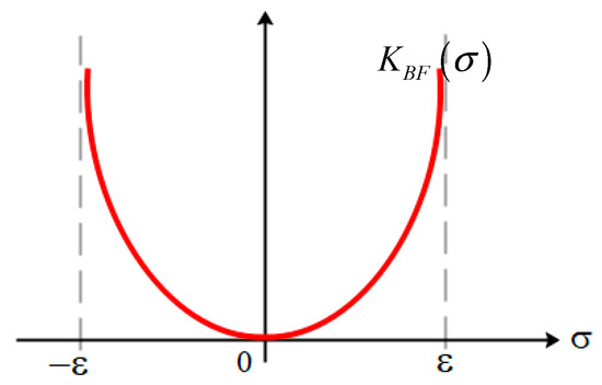
Figure 1.
Barrier function
For the presented adaptation algorithm, the following BF is used,
The course of the Barrier Function is presented in Figure 1.
For the adaptation algorithm and chattering suppression, the quasi BF-QFB, is proposed. The main property of the is
The quasi Barrier Function is defined as
where the is defined as
The QBF is presented in Figure 2.
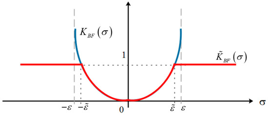
Figure 2.
Quasi barrier function
The adaptive STA controller with QFB adaptive coefficients (BSTA) is given as [23]
The feedback system with BSTA is
For the stability proof of the BSTA adaptation procedure, we assumed that the sliding variable at the time , is in the boundary of , where is and .
Let us consider the Lyapunov Barrier Function ,
The time derivative of is
For further derivation, we take the and . The time derivative is
Defining
yields
The upper bound of the Lyapunov function derivation is
where
The convergence and stability of the BF adaptation approach are ensured if the is a strict positive semidefinite function; . From the expression Equations (25)–(27), it is obvious that the stability of the system is ensured if the sliding variable is smaller than the BF boundary . If the variable is getting closer to the , then the function converges to zero, and the expression Equation (27) holds if . The stability proof for BSTA is finished. In the presented paper, BF is used for chattering alleviation; therefore, the BF operation boundary is limited to the pre-selected value , Figure 2, where the chattering alleviation starts and holds, . For the smooth transition from STA to BSTA, or operation mode one to two, and, with regards to Figure 2 and Equation (19), the gain of Equation (20) needs to be selected as
The boundaries and are design parameters. The execution procedure of BSTA is shown as a pseudocode in Algorithm 1.
| Algorithm 1 BSTA execution procedure |
|
The closed-loop system with BSTA and Algorithm 1 is shown in Figure 3.
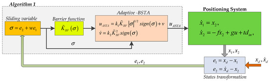
Figure 3.
Closed-loop system with the BSTA controller.
5. Results
The simulations and experimental results will be assessed in this section. We will compare the control strategy with STA and the BSTA controller. Both controllers have the same values of the parameters and obtained according to the stability proof from Section 3, whereby the BSTA controller deploys the BF adaptation algorithm described in Section 4. The implementation strategy for STA is simpler, but BSTA achieves good chattering alleviation, where the performance and accuracy of the closed loop remain unchanged. For the experimental results, the positioning system was used with the given parameters. All the parameters are taken from the nameplate of the positioning system manufacturer. Used parameters for the positioning system are presented in Table 1.

Table 1.
The parameters of the positioning system.
The parameters for controllers are selected regarding the conditions of Equations (16) and (27). The unknown disturbance term is assumed to be bounded with the value . The control objectives are the complete rejection of the disturbance term, robustness to system parameter variation, smooth controller output and good reference tracking capability, as well as the settling time for the shaft revolution, which need to be less than 4 s. The select controller parameters, with regard to the close-loop requirements, are presented in Table 2.
Table 2.
STA and BSTA controllers’ parameters.
In order to evaluate the control performance, we have considered three indices, defined as follows,
where , , are a number of samples, root mean square value (RMS) for motor angle, sliding variable, and STA controller output, respectively.
5.1. Simulation Results
The simulation was performed by the Feedforward integration technique for the plant discretization and preselected solver-integration time, . The controller sampling time in the simulation, as well as in the experimental environment, was selected as, . Figure 4 and Figure 5 show the simulation results of the comparison between STA and BSTA controller techniques. For more realistic simulation, the measurement noise was added to the angle and velocity variable. The power spectra of the added Gaussian noise was 0.32.
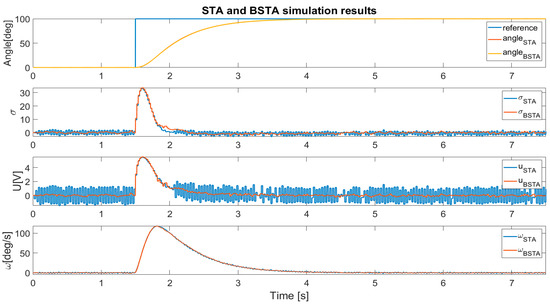
Figure 4.
Comparison of the STA and BSTA control algorithms.
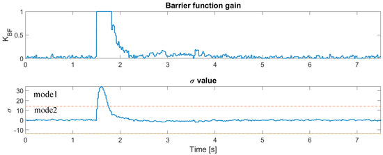
Figure 5.
Comparison of the STA and BSTA control algorithms.
The RMS values of the variables with regard to the measurements of Equation (29).
The simulation results prove that the BSTA algorithm has a much smaller chattering phenomena at the output, although the dynamic of the closed-loop system remains the same. The efficiency of the BSTA system is improved, which can be seen clearly in Table 3, where the RMS values are presented. It is also worth mentioning that the BSTA algorithm is less sensitive to the preselected sampling time of the discrete implementation.
Table 3.
The root mean square (RMS) values of the variables , , .
5.2. Experimental Results
Real-time experiments were performed on the ARM STM32F4xx system with a digital signal processing unit and internal clock of 167 MHz. The angle and velocity of the system are measured with a rotary encoder with 3200 positions per revolution. The sampling time of the controller is the same as in the simulation experiment. For the aim of the comparison and validation of the proposed algorithm, the input disturbance is generated at the output of the BSTA controller. The span of the disturbance is selected in such a manner that the requirements of STA stability are fulfilled. For experimental testing, the disturbance is selected as , which is 10% of the allowed input voltage. The real-time experiment structure with generated disturbance is depicted in Figure 6.
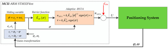
Figure 6.
Real-time experiment structure with disturbance.
Figure 7 presents the real-time experiment of the positioning system with the STA controller.
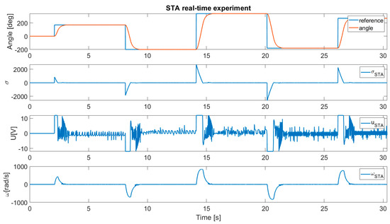
Figure 7.
System response with the STA algorithm.
Figure 8 shows the results of the closed-loop system with the BSTA algorithm.
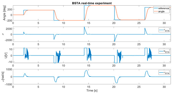
Figure 8.
System response with the BSTA algorithm.
Figure 9 presents the value of the function and a closer view of the sliding variable with the BF adaptation boundary.
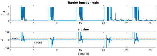
Figure 9.
Barrier function value and adaptation boundary of the BSTA coefficients.
Figure 10 presents the comparison between STA and BSTA, with real-time experiments’ data.
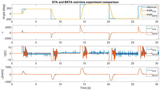
Figure 10.
Barrier function value and adaptation boundary of the BSTA coefficients.
The RMS values Equation (29) of the variables calculated from the real-time experiment are given in Table 4.
Table 4.
The RMS values of the real-time experiment of the variables , , .
The tracking capability of the BSTA compared to the STA remained unchanged, which can be confirmed by the value in Table 4. It can be noticed that the controller output value is notably reduced, and the value of BSTA is remarkably smaller. After the tracking capability test, the disturbance suppression ability needs to be inspected. For the real-time experiment, the input disturbance is added to the system. For the given disturbance experiment, the input disturbance amount is 34% of the whole controller output span, and the stepwise function was used.
Figure 11 shows the STA’s capability of disturbance suppression.
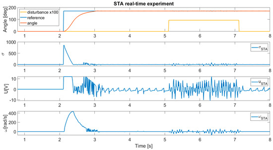
Figure 11.
Disturbance rejection of the STA controller.
Figure 12 presents the reaction of the BSTA with disturbance.
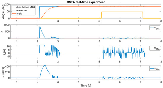
Figure 12.
Disturbance rejection of the BSTA controller.
Figure 13 shows the values of the function and closer view of the adaptation boundaries.
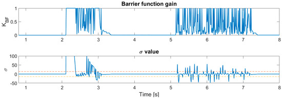
Figure 13.
Barrier function value and adaptation boundary of the BSTA coefficients with disturbance.
Figure 14 presents the comparison between the STA and BSTA algorithms with disturbance.
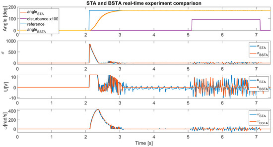
Figure 14.
Comparison of the STA and BSTA with disturbance.
Figure 15 shows a closer view of the section where disturbance was present.
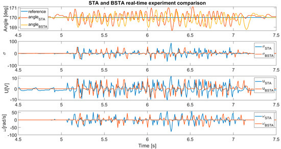
Figure 15.
Closer view of the disturbance rejection capability of the STA and BSTA algorithms.
values for the disturbance rejection capability are presented in Table 5.
Table 5.
The RMS values of the real-time experiment with disturbance of the variables , , .
From the simulation results in Figure 5; Figure 6, it can be concluded that the BSTA algorithm outperforms the standard STA. There is a significant difference in chattering phenomena alleviation. The efficiency of the BSTA gain adaptation can be seen clearly in Figure 6, where the chattering phenomena are effectively suppressed. It needs to be mentioned that the adaptation method with BF decreases the BSTA controller coefficients and, consequently, the output of the controller; therefore, the system dynamics were not changed noticeably. That can be confirmed straightforwardly with the RMS values of the system output and sliding variable in Table 3. The real-time experiment offers the same conclusion, which can be seen in Figure 6, Figure 7, Figure 8, Figure 9, Figure 10, Figure 11, Figure 12, Figure 13, Figure 14 and Figure 15. The BSTA has good chattering suppression capability and the same closed-loop performance as the STA. Also, the real-time experiment confirms that the BF adaptation process leads the controller output to lower values, with remarkably lower power consumption and higher efficiency of the system. This can be confirmed by the in Table 3; Table 4. For the positioning system, it is also very important to reduce the chattering phenomena in order to lower the system wear, due to the excessive small mechanical movement of the system, which is produced by the harsh and non-continuous controller output. The chattering phenomena also produce a power dissipation on the positioning system drive and increase the heat loss, which is closely related to the power efficiency of the system. The disturbance suppression capability of the BSTA is preserved, and remains the same as on the STA, which can be seen in Figure 11, Figure 12, Figure 13, Figure 14 and Figure 15. In the presented experiment, the chattering phenomena are also caused by the digital implementation of the algorithm. The discrete implementation of SMC is called the quasi-sliding mode, and the chattering phenomena are proportional to the sampling period [34]. In the experimental results, the influence of the sampling time is effectively reduced.
6. Conclusions
A novel developed chattering suppression technique for the positioning system is presented in this paper. The main issue with the SMC controller is unwanted non-linear and fast-changing controller output, which have a common name: chattering phenomena. The presented work proposes a chattering alleviation technique with the Barrier Function. In the presented results, the methodology offers promising results, efficiently improving the smoothness of the SMC controller output. The approach can be also used in the HOSMC, as well as on FSMC controllers. The complexity of the BSTA controller is increased compared to the non-adaptive version, but the computational burden is inattentive. Compared to the other adaptation, the SMC technique, BF is simpler and very efficient. The only tuning parameter is the adaptation boundary, which influences the closed-loop dynamic disturbance rejection capability and chattering alleviation directly. The boundary needs to be selected experimentally and is a trade-off between dynamic disturbance performance and chattering alleviation.
There is a lot of possibility for improvement and adaptation. The first question is how to select the STA parameters optimally. The initial value of the STA parameters influences the convergence time of the BF adaptation. The BSTA controller can be improved with an additional adaptation procedure, which can be used for STA parameter selection based on the disturbance estimation [35]. There is also the possibility of adaptive BF boundary tuning in operation mode two. The adaptive boundary can be changed according to the change in the reference signal. When the reference signal is changed by a certain value, the adaptation boundary can be increased or decreased, with the aim of ensuring a proper closed-loop dynamic or reducing chattering phenomena. Such an adaptation approach would be appropriate for time-varying or periodic reference signals.
Author Contributions
Methodology A.S. and R.S., conceptualization R.S. and D.G., validation D.G., writing A.S. and R.S., editing D.G., simulation R.S. and A.S., implementation A.S. All authors have read and agreed to the published version of the manuscript.
Funding
This research was supported by the Slovenian Ministry of Education, Science, and Sport under Grant number P2-0065.
Conflicts of Interest
The authors declare no conflict of interest.
References
- Kong, K.; Tomizuka, M. Nominal model manipulation for enhancement of stability robustness for disturbance observer. Int. J. Control Autom. Syst. 2013, 11, 12–20. [Google Scholar] [CrossRef]
- Sarjaš, A.; Svecko, R.; Chowdhury, A. Strong stabilization servo controller with optimization of performance criteria. ISA Trans. 2011, 50, 419–431. [Google Scholar] [CrossRef] [PubMed]
- Sarjaš, A.; Svecko, R.; Chowdhury, A. An H∞ Modified Robust Disturbance Observer Design for Mechanical-Positioning Systems. Int. J. Control Autom. Syst. 2015, 13, 575–586. [Google Scholar] [CrossRef]
- Kobayashi, H.; Katsura, S.; Ohnishi, K. An analysis of parameter variations of disturbance observer for motion control. IEEE Trans. Ind. Electron. 2007, 54, 3413–3421. [Google Scholar] [CrossRef]
- Zhou, L.; She, J.; Min, W.; He, Y. Design of a robust observer-based modified repetitive-control system. ISA Trans. 2013, 52, 375–382. [Google Scholar] [CrossRef]
- Moreno, J.A.; Osorio, M. Strict Lyapunov functions for the super-twisting algorithm. IEEE Trans. Autom. Control 2012, 57, 1035–1040. [Google Scholar] [CrossRef]
- Chalanga, A.; Kamal, S.; Fridman, L.; Bandyopadhyay, B.; Moreno, J.A. Implementation of super-twisting control: Super-twisting and higher order sliding-mode observer-based approaches. IEEE Trans. Ind. Electron. 2016, 63, 3677–3685. [Google Scholar] [CrossRef]
- Ventura, U.P.; Fridman, L. When is it reasonable to implement the discontinuous sliding-mode controllers instead of the continuous ones? Frequency domain criteria. Int. J. Robust Nonlinear Control 2018, 29, 810–828. [Google Scholar] [CrossRef]
- Ventura, U.P.; Fridman, L. Design of super-twisting control gains: A describing function based methodology. Automatic 2019, 99, 175–180. [Google Scholar] [CrossRef]
- Shtessel, Y.; Edwards, C.; Fridman, L.; Levant, A. Sliding Mode Control and Observation; Birkhäuser: Secaucus, NJ, USA, 2014. [Google Scholar]
- Utkin, V. Discussion aspects of high-order sliding mode control. IEEE Trans. Autom. Control 2016, 61, 829–833. [Google Scholar] [CrossRef]
- Tseng, M.L.; Chen, M.S. Chattering reduction of sliding mode control by low-pass filtering the control signal. Asian J. Control 2010, 12, 392–398. [Google Scholar] [CrossRef]
- Burton, J.A.; Zinober, A.S.I. Continuous approximation of variable structure control. Int. J. Syst. Sci. 1986, 17, 875–885. [Google Scholar] [CrossRef]
- Shtessel, Y.; Taleb, M.; Plestan, F. A novel adaptive gain super-twisting sliding mode controller: Methodology and application. Automatica 2012, 48, 759–769. [Google Scholar] [CrossRef]
- Utkin, V.I.; Poznyak, A.S. Adaptive sliding mode control with application to super-twist algorithm: Equivalent control method. Automatica 2013, 49, 39–47. [Google Scholar] [CrossRef]
- Negrete-Chavez, D.Y.; Moreno, J.A. Second-order sliding mode output feedback controller with adaptation. Int. J. Adapt. Control Signal Process. 2016, 30, 1523–1543. [Google Scholar] [CrossRef]
- Feng, Z.; Fei, J. Design and analysis of adaptive Super-Twisting sliding mode control for a microgyroscope. PLoS ONE 2018, 13, e0189457. [Google Scholar] [CrossRef]
- Krzywanski, J.; Wesolowska, M.; Blaszczuk, A.; Majchrzak, A.; Komorowski, M.; Nowak, W. The Non-Iterative Estimation of Bed-to-Wall Heat Transfer Coefficient in a CFBC by Fuzzy Logic Methods. Procedia Eng. 2016, 157, 66–71. [Google Scholar] [CrossRef]
- Błaszczuk, A.; Krzywański, J. A comparison of fuzzy logic and cluster renewal approaches for heat transfer modeling in a 1296 t/h CFB boiler with low level of flue gas recirculation. Arch. Thermodyn. 2017, 38, 91–122. [Google Scholar] [CrossRef]
- Boiko, I.; Fridman, L. Analysis of chattering in continuous sliding mode controllers. IEEE Trans. Autom. Control 2005, 50, 1442–1446. [Google Scholar] [CrossRef]
- Ventura, U.P.; Fridman, L. Chattering measurement in SMC and HOSMC. In Proceedings of the 2016 14th International Workshop on Variable Structure Systems, Nanjing, China, 1–4 June 2016; pp. 108–113. [Google Scholar] [CrossRef]
- Tee, K.P.; Ge, S.S.; Tay, E.H. Barrier lyapunov functions for the control of output-constrained nonlinear systems. Automatica 2009, 45, 918–927. [Google Scholar] [CrossRef]
- Obeid, H.; Fridman, L.; Laghrouche, S.; Harmouche, M.; Golkani, M.A. Adaptation of Levant’s differentiator based on barrier function. Int. J. Control 2017, 9, 2019–2027. [Google Scholar] [CrossRef]
- Castillo, I.; Freidovich, L. Barrier Sliding Mode Control and On-line Trajectory Generation for the Automation of a Mobile Hydraulic Crane. In Proceedings of the 2018 15th International Workshop on Variable Structure Systems (VSS), Graz, Austria, 9–11 July 2018; pp. 162–167. [Google Scholar] [CrossRef]
- Obeid, H.; Fridman, L.; Laghrouche, S.; Harmouche, M. Barrier Function-Based Adaptive Sliding Mode Control. Automatica 2018, 93, 540–544. [Google Scholar] [CrossRef]
- Utkin, V.; Guldner, J.; Shi, J. Sliding Mode Control in Electromechanical Systems, 2nd ed.; CRC Press: Boca Raton, FL, USA, 2009. [Google Scholar]
- Golkani, M.A.; Koch, S.; Reichhartinger, M.; Horn, M. A novel saturated super-twisting algorithm. Syst. Control Lett. 2018, 119, 52–56. [Google Scholar] [CrossRef]
- Moreno, J.A.; Osorio, M.A. Lyapunov approach to second-order sliding mode controller and observer. In Proceedings of the 47th IEEE Conference on Decision and Control, Cancun, Mexico, 9–11 December 2008; pp. 2856–2861. [Google Scholar]
- Bartolini, G.; Ferrara, A.; Pisano, A.; Usai, E. Adaptive reduction of the control effort in chattering-free sliding-mode control of uncertain nonlinear systems. Appl. Math. Comput. Sci. 1998, 8, 51–71. [Google Scholar]
- Incremona, G.P.; Cucuzzella, M.; Ferrara, A. Adaptive suboptimal second-order sliding mode control for microgrids. Int. J. Control 2016, 89, 1849–1867. [Google Scholar] [CrossRef]
- Plestan, F.; Shtessel, Y.; Bregeault, V.; Poznyak, A. New methodologies for adaptive sliding mode control. Int. J. Control 2010, 83, 1907–1919. [Google Scholar] [CrossRef]
- Obeid, H.; Fridman, L.; Laghrouche, S.; Harmouche, M. Barrier Function-Based Adaptive Integral Sliding Mode Control. In Proceedings of the 47th 2018 IEEE Conference on Decision and Control, Miami Beach, FL, USA, 17–19 December 2018; pp. 5946–5950. [Google Scholar]
- Christopher, E.; Shtessel, Y.B. Adaptive continuous higher order sliding mode control. Automatica 2016, 65, 183–190. [Google Scholar]
- Zhang, J.; Youngkai, L.; Shijie, G.; Chengshan, H. Control Technology of Ground-Based Laser Communication Servo Turntable via a Novel Digital Sliding Mode Controller. Appl. Sci. 2019, 9, 4051. [Google Scholar] [CrossRef]
- Mehgsji, Z.; Jian, H.; Yu, C. Adaptive Super-Twisting Control for Mobile Wheeled Inverted Pendulum Systems. Appl. Sci. 2019, 9, 2508. [Google Scholar]
© 2020 by the authors. Licensee MDPI, Basel, Switzerland. This article is an open access article distributed under the terms and conditions of the Creative Commons Attribution (CC BY) license (http://creativecommons.org/licenses/by/4.0/).