Abstract
Modern approaches to physical therapy often use electric currents induced by time-varying magnetic fields. Although some of these methods are already commonly used, and only a few studies are looking at applying particular techniques on exposed tissue. In this study, a high-induction magnetic stimulation (HIMS) was applied to the chest area to affect the electrical conduction system of the heart. The animal model Sus scrofa domesticus was used for the study. Standard methods were used to make the subsequent analysis, i.e., heart rate variability in time and frequency domain. Concerning the nonlinear character of the electrocardiographic signal and evaluating complex variability (complexity), recurrent quantification analysis was used. The results show high resistance to a physiologically working heart, but there are also specific changes concerning complex variability. Thus, the results indicate that the HIMS application in the chest area may not pose a significant risk to healthy individuals in terms of the short-term effect of this technique on cardiac activity. However, cardiac activity is still, to some extent, affected by the HIMS application. In view of this and the fact that the study was conducted on an animal model, further research in this area would be appropriate.
1. Introduction
With every scientific progress, numerous methods of physical therapy are being tested and applied, including magnetic therapy. Commonly used devices produce a non-stationary, time-varying, magnetic field. Such devices differ with set parameters, intended use and design. In most cases, the time-varying pulsed magnetic flux is used. To date, the effect of either time-varying or stationary magnetic field remains questionable. Although there is no consensus on whether such devices have a positive impact on biological tissues, there have been scientific studies that indicate a positive influence of induced electric field [1,2].
Past decades have showed the importance of the low-frequency electromagnetic field as a means in physical treatments used in the field of physical medicine and physiatry, the use of which is also supported by recent findings [3,4,5]. Rarely, an alternating current waveform with frequencies from the ELF (extremely low-frequency) band is applied. Whether the biological tissues are conductive or not, the time-varying magnetic field induces an electric field. After the electric field is induced in conductive tissues, the electric charge is carried by charge carriers such as ions. Factors such as the current density of induced electric current have proven to have an effect on tissue treatment because it also has the character of physical energy. The bounce of the induced electrical voltage is caused as a result of a rapid and specifically defined change in time of the high-intensity magnetic field, ergo causing the bounce of induced magnetic electric current (formed in the manipulated/treated tissues). Current densities of the order of tens to hundreds of induced in such magnetic field have the required therapeutic ability to affect the sensational and locomotive system [6].
Specific stimulation is achieved by currently available technologies on the medical devices market. Sensory neural pathways are activated due to the application of the magnetic field. This fact causes the sensitivity threshold to be exceeded [7]. Perceived nociception is only minimal due to very specific stimulation, although the afference is very strong in the treated area. Many remedial theories are linked to the evoked afference such as the local trophic effect, a response of neurophysiological mechanisms in segmented and distant polysynaptic reflexes. This fact provides the magnetotherapy (not only) with an analgesic effect, but if applied locally, it also causes the improvement of blood flow and lymphatic functions in treated tissues. In the case of distant application of the magnetic field, treated tissues are affected by the autonomic nervous system network, specifically by the sympathetic nervous system. Nerves restoration in denervated areas and the recovery of damaged or injured tissues is accomplished/facilitated by the afference and its succeeding efference due to the application of the magnetic field [8,9].
The high-induction magnetic stimulation (HIMS) attracts considerable interest due to its significant impact in a short time, i.e., for the time of the HIMS application procedure. HIMS triggers motor effects through contractions in muscle fibers, without the device touching treated area of muscles [10]. Denervated muscles suffer from atrophies and paralyzes. Still, the stimulation of the motoric system can stop further muscle loss. Recent findings regarding the high-induction magnetic stimulation indicate that it is an effective treatment of functional immobilization initiating the atrophy of particular muscles or whole muscle groups as well as pareses and plegia of organical origins. The high-induction magnetic stimulation has proven to have a great treatment impact on hypertonic muscle spasms and muscle spasticity in general. In fact, HIMS could affect hypertonic muscles to relax and thus, decrease muscle spasticity [1,4,11,12].
As previously outlined, pathologies in the locomotor system varying from minor to degenerative (structural) disorders and paralyzes [13], treating perfusion pathologies [14], are assumed to be treated by the HIMS. A notable benefit of the HIMS application is that it is a much quicker procedure than magnetic pulse therapy, distance electrotherapy, or other physiological treatment.
Within the next few years, HIMS is likely to become an important therapeutic treatment in physical medicine and rehabilitation. However, despite the procedure’s advantages, there are several hazards linked to the powerful magnetic field. There are several situations when it is unsafe to undergo such procedure—subjects with an implant in the area of magnetic field application, with a cardiac stimulator, being pregnant, etc. In fact, current studies have not proved other significant contraindications. High-induced current density could affect the autonomous regulation of the heart activity and influence the electrical conduction system of the heart when applied in the thoracic or near-thoracic area. The safety of the application of the magnetic field in the chest area has (so far) been neglected. Therefore, the effects remain unclear whether and how the magnetic field affects the biophysical stimulation from the safety point of view.
Regarding monitoring and evaluating of cardiac activity or its influencing by HIMS application is necessary to choose a suitable method. The heart rate variability (HRV) is considered to be an indicator of the activity of the autonomous nervous system. First studies were carried out already in the 1960s, and since then, the clinical impact of HRV was a subject of various research. It is well known that by choosing a suitable analysis of the HRV, we can get a picture of sympathovagal balance. For these reasons, the analysis of HRV is also used in clinical applications for cardiac activity evaluation. Therefore, there are standard procedures regarding the HRV, but not only for the purpose of how to perform analysis but also how to make records [15]. Based on the available studies, we can claim that HRV is a suitable indicator of both the autonomous nervous system as well as pathological conditions [15].
The aim of this study is to examine and analyze the cardiac activity, to be precise, the ECG signal. Variation of heartbeats interval, the Heart Rate Variability (HRV) will be evaluated during the HIMS application in the chest area of an animal model. The biophysical stimulation before, during, and after the HIMS application is going to be analyzed by standard HRV evaluation methods, such as time and frequency domain. In addition to the standard approach to the HRV assessment and the results interpretation, an evaluation by nonlinear methods is going to be included. The assessment is important to evaluate not only the heart rate variability but also its complexity. The reason for the evaluation is that it appears that the most complex signals are generated by organisms that are in their most adaptive (healthy) state. The complexity of a signal relates to its structural richness and correlations across multiple time scales [16].
Current methods focus on the use of nonlinear evaluation methods such as Poincaré plot (a short-term and long-term variability dependency of the monitored time series) [17], an investigation of entropy [16,18], a use of detrended fluctuation analysis or other methods of symbolic dynamics analyses [18]. Such methods evaluate the unpredictability of the time series emerging from the complexity of mechanisms regulating the HRV. Nonlinear parameters relate to specific measurements in the time and frequency domain. These parameters are described in more detail in [19].
Especially in medical research, the use of nonlinear signal analysis, which is based on the reconstruction of trajectory in phase space, is increasing. Methods based on the phase space reconstruction are quite recent—their development is linked to the delay embedding theorem discovered by the mathematician Takens [20] in 1981. Recurrence quantification analysis is one of the nonlinear methods based on the chaos theory [21].
The recurrence quantification analysis enables visualization of the recurrence of dynamic systems (for more see [21,22,23]). to visualize the recurrence one data set of time series is needed. No requirements such as length, stationarity or distribution are imposed on the time series data set [23]. The recurrence quantification analysis is a multidimensional method which allows monitoring the dynamics of a whole system [23].
Based on the above mentioned, standard assessment methods in time and frequency domain will be used to research the influence of the HIMS on the regulation of the cardiac activity. Moreover, the standard assessment methods, the basic nonlinear methods and recurrence quantification analysis will be used to describe the monitored system dynamics.
2. Materials and Methods
2.1. Subjects
The experimental verification of the safety of the high-induction magnetic stimulation and its direct effect on cardiac activity was carried out on the animal model Sus scrofa domesticus. The frontal part of the thoracic cage was selected as an area of application, see Figure 1.
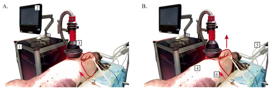
Figure 1.
Sus scrofa domesticus without muscle contraction (A) and with muscle contraction (B) during the application of high-induction magnetic stimulation procedure (1—high-induction magnetic stimulation device, 2—control and indicative display, 3—applicator, 4—Sus scrofa domesticus, 5—anesthesia and intubation equipment, 6—electrocardiograph electrode).
The animal was handled following the European Directive for the Protection of Vertebrate animals Used for Experimental and Other Scientific Purposes (86/609/EU). The experiments were approved by the Committee for Experiments on animals of the Charles University Faculty of Medicine in Pilsen. Nine domestic piglets (Prestice Black-Pied pigs) of both sexes and of similar weight (25–40 kg) were used for experiments. After premedication with i.m. Atropine (1 mg), ketamine 200 mg (5–10 mg·kg) and azaperone 160 mg (2–8 mg· kg), general anesthesia was induced by continuous administration of propofol and fentanyl through a peripheral or central venous catheter in the following total average doses: propofol (1% mixture 5–10 mg·kgh) and fentanyl (1–2 g·kgh). In general, anesthesia is associated with an inhibition of the autonomic nervous system and, consequently, of heart rate variability. Effects of fentanyl and propofol used for anesthesia in this study were repeatedly addressed in patients, and a reduction of overall autonomic nervous system modulation, perhaps with dominant inhibition of sympathetic branch, was found [24,25,26]. However, since in this study, the entire experiment was performed under stable deep anesthesia, we assume that although the absolute levels of heart rate variability may differ between conscious and anesthetized animals, the pattern of HRV changes induced by HIMS should be similar.
Electrocardiogram (lead II) was recorded continuously throughout the entire experiment using a Biopac system (Biopac Systems, Inc., Goleta, CA, USA). At the same time, the ECG record was sampled with a sampling rate of 512 Hz.
2.2. Experimental Setup and Data Acquisition
A contactless magnetic stimulation device SALUTER MOTI (Embitron, Ltd., Vochov, Czech Republic) was used for the purpose of this study. This device is designed to target deep and large muscles and axons in plexuses, organs, and tissues. The parameters of the stimulative magnetic field are enabling activation of sensory neural pathways by which a sensitivity threshold is exceeded. However, this device generates a very specific stimulation ensuring that the perception of nociceptive pain is provoked only minimally. The SALUTER MOTI instrument produces high-quality, nonpainful, exceptionally strong and deep high-induction magnetic stimulation of a wide range of frequency modulations.
SALUTER MOTI device meets basic requirements of the Medical Device Directive EU 93/42/EEC laying down technical requirements for medical devices as amended and in accordance with applicable technical standards and regulations. The properties, type, nature, and parameters of the medical device correspond with the intended use and are in line with current clinical knowledge.
The technical solution is based on a controlled resonant circuit producing high-current impulses generating strong and time-varying magnetic fields around a special applicator. Actuation and indication are ensured by a control computer with a touchscreen. Apart from the device’s number of preprogrammed procedures, it also offers the possibility to customize the procedure parameters according to the patient’s specific needs and medical prescription.
With the use of the described device, the setup for HIMS was characterized by generating 0.5 Hz pulses (see Figure 2) for a magnetic induction of 2.5 T, resulting in an induced current of 270 A/m. The procedure took 3 min (a total of 90 pulses). The aim was to influence the electrical conduction system of the heart with perspective ventricular fibrillation. However, this effect was not observed during or after the procedure. In addition to the predicted contraction of M. pectoralis), no pathological change in cardiac activity was found in the area of application, according to the ECG record (see Figure 2).
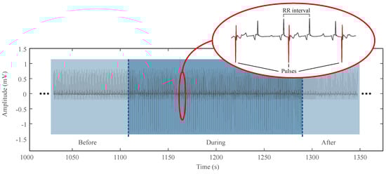
Figure 2.
Example of electrocardiogram during high-induction magnetic stimulation procedure with detailed ECG curve with applied pulses.
The above mentioned was the reason for performing a more in-depth heart rate variability analysis. This analysis was performed by using standard evaluation methods of RR interval time series. As a reference time series for the evaluation, a 5-min segment before the procedure was compared with a 5-min segment after the procedure. At first, the application data had to be filtered. By knowing the frequency of applied pulses, individual pulses were filtered out. At the same time, it was necessary to supervise the execution of data filtering to prevent the loss of information regarding the cardiac activity, i.e., loss of the detected R-waves. Therefore, individual signals were filtered by the finite impulse response (FIR) filter due to their linear phase characteristic. We used a notch filter with limiting frequencies 0.3 and 0.7 Hz to eliminate the 0.5 Hz part.
2.3. Data Processing and Data analysis
From the cardiac activity pre-processed records with a 0.5Hz component filtered, we separated three sections of corresponding segments of measurements, one before the HIMS application (Group A), one during the HIMS application (Group B), and one after the HIMS application (Group C). All records had the same length. Subsequently, we used the Pan-Tompkins method to identify the R-waves [27]. Furthermore, we obtained individual RR interval vectors, i.e., time intervals between individual R-waves. We processed collected data sets of RR intervals by standard methods, i.e., time-domain analysis, and frequency analysis [19] and by nonlinear analysis—The Recurrence quantification analysis (RQA) [28].
Concerning the time-domain analysis, parameters of mean RR interval (meanRR) and mean heart rate values (meanHR) were obtained. In this case, these are the standard arithmetic means of the given parameters. Moreover, we got long-term variability parameters through the standard deviation of NN (normal-to-normal) intervals (SDNN) and the standard deviation of heart rate (SDHR) [19]. The number of adjacent RR intervals differing by more than 50 ms (NN50), the number of such intervals to the total number of RR intervals (pNN50), and Root mean square of successive RR interval differences (RMSSD) were selected as further parameters. These parameters are used for longer signals [19] but are stated to get the complete standard analysis.
Frequency analysis uses the power spectral density (PSD), which is based on the conversion of signals into the frequency spectrum using a Fourier transform (FT), or more precisely, a Discrete Fourier transform (DFT) because of the discrete signal. Standard FT, or rather DFT, considers an equidistantly sampled signal. Thus, in the case of HRV, this requirement is not met. For this purpose, a so-called Lomb periodogram is used, which was developed for the modification of non-equidistantly sampled data. The acquired power spectrum of HRV is then divided into frequency bands, each of which is associated with different functional effects on RR intervals [29].
In the case of the frequency analysis, outputs in individual frequency bands defined for HRV in the range of low frequencies (LF), i.e., absolute power of low-frequency band (0.04–0.15 Hz) and in the band of high frequencies (HF), i.e., absolute power of the high-frequency band (0.15–0.4 Hz), were monitored. An LF and HF ratio (LF/HF) was obtained by mentioned parameters, and it is used as an indicator of sympathovagal balance, i.e., a balance indicator of the sympathetic and parasympathetic activity of the neural system [19].
Given the nonlinear nature of biological signals, data were further evaluated using the method based on the chaos theory method—the RQA, described further [28].
Monitored parameters, or more precisely, their values were statistically compared before and after the HIMS application. We rejected the null hypothesis of normal distribution based on the Jarque–Berra test [30]. Regarding the rejection and the fact that paired data were compared, a Friedman test, which is the non-parametric alternative to the one-way ANOVA with repeated measures and post-hoc analysis (Dunn and Sidak’s approach [31]), was carried out to statistically compare the state before, during and after the HIMS application [32]. Statistical significance is presented in the form of p-values, where indicates a statistically significant difference between compared groups because data were tested at the significance level of . Individual p-values represent the result of Friedman’s test. The p-value indicates that there is a statistically significant difference between the pairs of study groups. However, the Friedman test itself does not determine between which particular pairs these differences exist. Therefore, mentioned post-hoc analysis was used. The results of the post-hoc analysis are presented in the form of confidence intervals providing complementary information which p-values are not able to. A null value indicates that the group means equal. If the confidence interval does not contain null, then compared groups are significantly different. The width of the interval shows how precise the estimation is —The narrower the width is, the higher is the precision [33]. Individual limits of confidence intervals are presented in the results further in the paper.
2.4. RQA
The first step is to create a multidimensional system relating to the original phase system. It is about the phase space reconstruction and the construction of a distance matrix (DM). Subsequently, points, although distant in time, but which are neighbors in space on a particular radius, are identified, and thus a recurrence plot (RP) is created. The last step is the quantitative assessment of RP—A recurrent quantification analysis (RQA) [28].
2.4.1. Phase Space Reconstruction
The trajectory in phase space represents the time development and system dynamics. With defined variables, every system is possible to describe. These variables form the trajectory in time and n-dimensional space, or precisely in the phase space [34].
In many cases, it is not possible to record or measure all the variables of the system’s state. The phase space, however, based only on one state variable, might be constructed. A widely and most frequently used method is an embedding dimension and time delay method by Dutch mathematician Takens, see equation below [34].
where u is observed state variable, is time delay and m is inserted dimension.
The reconstructed phase space does not entirely match the original phase space, but in case that the inserted dimension is sufficiently large, its topological properties remain the same [34]. The inserted dimension should be at least twice the size of the attractor’s dimension, precisely [34,35]. There are several opinions on the input parameters (dimension, time delay) setup. The optimal setup of these parameters is important when reconstructing the phase space, which will fully depict system dynamics.
Time delay sets the distance between neighboring elements. If the value of time delay was too big, the states of reconstructed phase space might appear independent, and thus the reconstructed trajectory will seem to be a random process. In contrast, if the value of time delay was small, the difference between individual states of the reconstructed phase space will be negligible.
In the past, to choose time delay, an autocorrelation function was used. Unfortunately, this method did not take into account the possibility of nonlinear processes [35]. Recent studies indicate that the method convenient for choosing the specific time delay is the mutual information [35,36]. The mutual information represents the information of mutual dependency of two dependent parameters. Higher mutual information means that the variables are more dependent on each other. The most suitable length of time delay is the first minimum value of mutual information. During the monitoring in time , on average the first minimum value presents the highest information contribution with regard to the information from the monitoring in time . The mutual information of two variables A and B might be defined through the entropy as:
where and are entropy and is joint entropy of A and B.
After the selection of the optimal time delay, it is necessary to choose the optimal dimension of an embedment. A frequently used method for selecting the optimal embedded dimension is a method of false nearest neighbors, and that is because of the fact that after projecting a system trajectory of the original phase space into space with low-dimension, there is a self-crossing of the trajectory. Because of the self-crossing, the false nearest neighbors, the number of which diminishes as the dimension increases, are formed. A disadvantage of using this method is that a threshold must be set to consider neighbors as false. An interesting modification of false nearest neighbors method that eliminates the mentioned disadvantage was described by Cao [37], who used the Euclidean quotient distances of two closest neighboring states in the dimension m and dimension , see Formula (3).
where is Euclidean distance, is the i-reconstructed vector of m and is the closest neighbor .
Furthermore, a variable called the average of all value is introduced [37]:
The average is dependent on dimension m and time delay . To determine the deviations of m from , the ratios of averages of the dimension m and dimension are also defined, see Formula (5) [37].
The value of the variable stops changing after the dimension m is greater than the value of the attractor’s dimension . The minimum value of the embedded dimension is then equal to [37].
2.4.2. Recurrence Plot
A trajectory visualization in phase space with more than three dimensions is challenging. Therefore, Eckmann [38] presented the so-called recurrence plots. These plots are a fundamental RQA tool that enables the visualization of multidimensional phase space in a two-dimensional plot. In the plot, the recurrence states recorded by “ones” are recorded in the matric format. Those states that are not recurrent are recorded with “zeros”. The recurrence state is possible to determine by the set threshold distance , see Formula (7). According to the [34], it is possible to express the recurrence plot as:
where is Heaviside function, can be a value 1 and 0 according to Formula (7):
where marks a point in a matrix R in time i and other time j, and are individual states of the system, N is the total number of states, is a distance of two states in a phase space and is a threshold distance [34].
A graphic representation of matrix R is the recurrence plot. Points with value 1 in the matrix represent the recurrence states. It is possible to encounter also a non-binary (colored) version of the recurrence plot, in which the distances in between the individual states (points) in the phase space are placed and, at the same time, the Heaviside function was not used. This procedure avoids entering a threshold distance, i.e., a graphic representation of the distance matrix. In the graph legend, there is a so-called colormap that defines what color corresponds to what distance.
A disadvantage of the recurrence plots is their mathematical complexity due to the paired t-test of all states. tests are counted for N states. In its very nature, the recurrence plot is always symmetrical, according to the main diagonal line. In addition, basic structures appear. These structures include separate points, diagonal lines, and vertical and horizontal lines, respectively. Each of these structures has its meaning [34].
Distant points represent unique points in the phase space, in which the system does not remain long. Diagonal lines mark the trajectories going through the same area in the phase space at a different time. Diagonal lines are characteristic of its determinism. Vertical and horizontal lines mark system remaining in one point or that might change very slowly [35]. Recurrence plot topology is depicted in Figure 3.
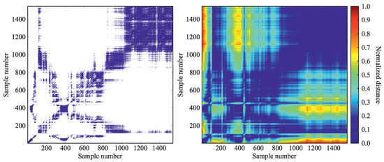
Figure 3.
Example of a recurrence plot (left) and a distance matrix (right).
The most important part when creating the recurrence plot is choosing the right threshold value. Recent studies discuss the optimal threshold value [39,40,41] because only the slightest change in threshold distance might dramatically affect the outcomes [40]. A frequently used method of setting the threshold distance is setting the threshold distance value percentually from the maximal distance in the phase space. Another used method focuses on such value that would not exceed 10% of the average or maximal distance in the phase space [39]. A fixed percentage of recurrence points is another method of setting the threshold value. To ensure this exact percentage of recurrence points, a certain threshold distance value is set [39]. Often, this value is 1% [39,40]. It is possible to see also different setting, e.g., 5% [42].
Other recommended settings include the threshold value ( is the standard deviation of signal input). This setting was set by Prof Marwan as a result of an experiment [41].
2.4.3. Quantitative Analysis of Recurrence Plots
So that the recurrence plots were not only a visual tool but would contribute with its evaluation apparatus, it is necessary to describe the parameters precisely and subsequently quantify them. Therefore, we used the recurrence quantification analysis, which was presented by Zbilut and Webber [21,43] and extended by Prof Marwan [22]. Lower, is a set of parameters describing the recurrence plot statistically.
The percentage of recurrent points is the percentage of recurrent points creating the plot. This parameter matches the probability that a particular state will repeat. Higher recurrence means lower system (sinus rhythm) variability and vice versa [23,35,42]:
Determinism is a parameter representing the percentage of recurrence points forming diagonal lines. This means that the system is getting back to previous states at a different time, i.e., increase of indicates the more frequent return of system (sinus rhythm) to previous states. The predictability of system dynamics and determinism parameter are linked to each other [23]:
where is a histogram of length of l diagonal lines.
The parameter represents the longest diagonal line. Its inverse value is then referred to as divergence . Shorter diagonal lines indicate a faster deviation of the phase trajectory segments, thus a higher degree of divergence (increase in the parameter). The L parameter, which represents the average length of the diagonal lines, is also used to supplement the system information [28]:
where is a histogram of length of l diagonal lines. Increase of and L or decrease of , indicate lower variability of the system (sinus rhythm), i.e., lower HRV.
Laminarity labels the percentage of points forming the vertical lines. This parameter is used to detect the laminar states, i.e., states when the system is changing or changes only very little [22,23]:
where is the histogram of length of v vertical lines.
The trapping time is a parameter that marks the average length of the vertical lines. The parameter labels the time—how long the system continues to stay in a specific state. In addition, it also contains information about the frequency and length of the laminar states [22,23]:
A low value of and labels the complex variability (complexity) of the system, i.e., complexity of sinus rhythm. The system returns to previous states only for a very short time [42]. The parameter, which represents the maximal length of the vertical lines and thus the maximum of all laminar state duration, is also used to indicate laminar states [22]. Increase of these three parameters then indicates that the system (sinus rhythm) stays in its previous state for a longer time which results in lower complexity.
One of the fundamental indicators of complexity is the Shannon entropy , defined by Formula [22]:
where [22]:
and is a number of diagonal lines in the recurrence plot. The increase of indicates higher information in system which means higher complexity [28]. Therefore, increasing the parameter increases system complexity while decreasing complexity reflects decrease and ability to further regulate cardiac activity is reduced system adaptability to external stimuli.
Trend () represents the RP drift towards its edges and is formulated as [22]:
where is maximal number of diagonals parallel to the line of identity (central diagonal) which will be considered for the calculation of . The is thus an indicator of system (sinus rhythm) non-stationarity [28]. Therefore, increasing values of indicated complexity of system (sinus rhythm) and values close to 0 reflects system homogeneity [44].
The last parameter is , which is the ratio between and . is used to detect specific transitions in the system, i.e., conditions where changes but the remains constant [28]. During physiological transitions, this parameter is increased, and then stabilized in the case of a quasi-stable state. Increasing the parameter thus indicates system transitions, i.e., transitions in sinus rhythm [21].
Based on what was already mentioned, the time delay was set automatically for each data set based on mutual information. The embedding dimension was also calculated separately for each dataset by using the method designed by Cao [37]. We set the threshold according to the fixed percentage of recurrent points in the resulting plot in a way that the resulting RR = 5 % (in reality, the value is around the mentioned value, so it is the closest possible value meeting the condition ).
3. Results
We used time, frequency, and recurrence quantification analysis to monitor the condition before, during, and after the HIMS application in the chest area. Results from the time-domain analysis provided us with 7 standard parameters used for the HRV analysis. Frequency analysis delivered additional 4 parameters relating to standard bands used in the HRV frequency analysis. The RQA delivered a total of 11 parameters relating to the structures occurring in the recurrence plot, and which describe the dynamics of the system.
To get statistics, we compared all the obtained parameters to monitor statistically significant differences in the state before, during, and after the HIMS application, see Table 1. Distribution of individual parameters among 3 datasets depicted in Figure 4, Figure 5 and Figure 6.

Table 1.
Result summary of Friedman’s test in the form of p-values along with results of post-hoc analysis, where the upper and lower limits of confidence intervals to compare the parameters monitored before and during (A-B), before and after (A-C) and during and after (B-C) the HIMS application are depicted.
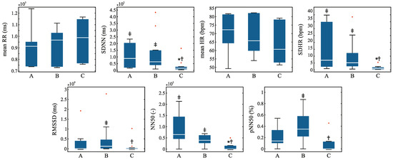
Figure 4.
Distribution of the time-domain HRV parameters before (A) during (B) and after (C) the HIMS application with highlighted outliers (red crosses). Symbol * means vs. group A, † means vs. group B, ‡ means vs. group C.
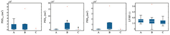
Figure 5.
Distribution of the frequency-domain HRV parameters before (A) during (B) and after (C) the HIMS application with highlighted outliers (red crosses). Symbol * means vs. group A, † means vs. group B, ‡ means vs. group C.
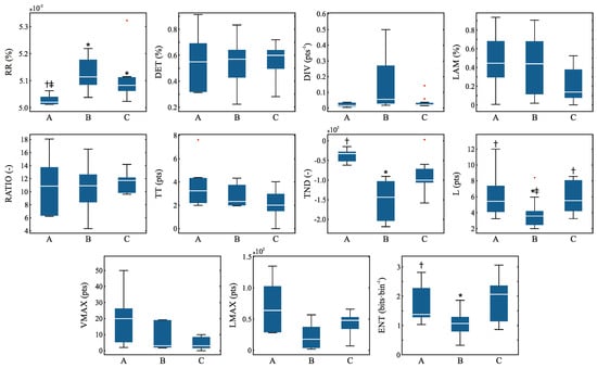
Figure 6.
Distribution of the recurrence quantification analysis parameters before (A) during (B) and after (C) the HIMS application with highlighted outliers (red crosses). Symbol * means vs. group A, † means vs. group B, ‡ means vs. group C.
The results show that in the case of time-domain analysis there was a significant change between the state before and after the application of HIMS in 2 parameters (SDHR, NN50), and then also between the state during and after the HIMS application in 5 parameters (SDNN, SDHR, NN50, pNN50, RMSSD). The distribution of the individual RQA parameters is shown in Figure 4.
Frequency analysis showed only one statistically significant transition, and that was in the low-frequency band between the state during and after the HIMS application. The distribution of the individual RQA parameters is depicted in the Figure 5.
The RQA showed statistically significant transitions between 4 parameters. The transition between the state before and during the HIMS application proved to be significant for 4 parameters—RR, TND, L, and ENT. A statistically significant difference between the before and after HIMS application was observed in the RR parameter. A significant difference between the state during and after the HIMS application was observed in the L parameter. The distribution of individual RQA parameters is shown in Figure 6.
4. Discussion
No pathological change in the ECG record was found by supervising physician during the measurement. This statement is also supported by the results where most parameters did not show a statistically significant difference between the compared time series. Therefore, there are no obvious changes in records before, during, and after the HIMS application.
However, in the case of long-term variability parameters, i.e., SDHR parameter, a statistically significant difference among data obtained before, during, and after the HIMS application was observed. Similarly, in the case of the RMSSD parameter, significant differences are observed. The RMSSD parameter is then linked to a short-term variability, i.e., variability between individual heartbeats [19]. Furthermore, significant differences were observed in the NN50 and pNN50 parameters, which also relate to variability [19]. Thus, it is becoming clear that the signal variability varied during the experiment, and therefore the HIMS application affects the variability of the heart rhythm in some way, although this is not obvious at first sight.
Looking at the results related to frequency analysis, it is evident that there are almost no significant transitions. The only significant transition had shown between the state during and after the HIMS application in the low-frequency band. This band is mainly related to parasympathetic activity [19]. We can declare, however, that it is not possible to form conclusions on influencing the heart rhythm of HIMS application based on the frequency analysis, and from the perspective of frequency analysis, it appears that the HIMS application may not have a more substantial influence on cardiac activity.
As was previously mentioned, biological processes are burdened with fluctuations, and therefore linear analysis does not seem to be an appropriate choice [45]. On the other hand, these results can be used as a baseline for further progress. By using the standard methods, it is possible to assume the influence on the variability of the heart rhythm through parameters that correspond to short and long-term variability. For these reasons, we carried out a recurrence quantification analysis.
The analysis is based on chaos theory and takes into account the nonlinear behavior of the signal [23]. In the case of the RQA, particularly transitions between states pre and during the HIMS application were observed. This was the case with the RR parameter, which indicates the variability of the system. The results show that in the case of the dataset with the application of HIMS, there is an increase of RR and, thus, a decrease of variability. Other transitions were found in the parameter L, representing the average time at which 2 segments in the phase space are close together [23], in the ENT parameter or rather Shannon entropy indicating the degree of chaos in the system [46], and finally in the TND parameter quantifying the stationarity of the system [23]. Taking into account the fact that RQA parameters are used as indicators of complexity, or in other words, complex variability [22], especially the ENT, it is clear that the HIMS application in the chest area can induce some changes in complexity. On the other hand, there were relatively few significant transitions, and it seems that the subjects’ hearts (i.e., hearts functioning without any pathologies) appeared to be highly resistant to the HIMS application.
The high resistance of the physiologically functioning electrical conduction system of the heart and the minimal possibility of affecting the operation of the sinoatrial node by low-frequency electromagnetic fields in a healthy heart is evident. The explanation for this phenomenon can be hypothetically found in the excellent electrical conductivity of the pectoral muscles as well as of the conductive serous fluids found between the pleura parietalis and the pleura visceralis, as well as between the pericardium and epicardium. These well-electrically conductive environments can concentrate a more significant part of the induced electrical currents, where their current paths can close, create a high-current density, and thus the heart itself can be largely shielded from the effect of the induced electrical currents. Another hypothesis is the idea of the “resilience” of the sinoatrial node and the entire electrical conduction system of the heart against the effects of external electromagnetic fields. It should be stressed, however, that these are the effects of an explicitly low-frequency, not the high-frequency impact of electromagnetic fields, known in physical medicine from the use of diathermy.
At the same time, however, certain changes can be observed based on complex variability. The results support the safety aspect of the high-induction magnetic stimulation but do not in any way imply that high-induction magnetic stimulation could be applied risk-free to the heart area where it is usually contraindicated, especially in cardiac patients or in risk patients. The presence of a pacemaker or other electronic surrogate in the body is a primary contraindication not only to the HIMS application but also to distance electrotherapy and any other application of induced electric currents and electromagnetic fields that could adversely affect the pacemaker or any other electronic surrogate with a fatal effect.
It is evident that at first look (and based on the basic descriptive statistics, i.e., meanRR and meanHR parameters), changes in cardiac activity are not apparent. Still, certain significant transitions show up in the parameters describing variability or complex variability (complexity). Therefore, we can say that although it seems that HIMS has no effect on the electrical conduction system of the heart based on the results of the fundamental analysis, the results indicate changes in variability, which decreases during or after the HIMS application. Therefore, it can be assumed that the HIMS application affects cardiac activity. Hence, there are changes in variability, but for more accurate results, it would be necessary to include a larger number of subjects in the study and possibly to extend the spectrum of applied pulses (with respect to their frequency).
5. Conclusions
High-induction magnetic stimulation is an effective form of electrotherapy without the need for galvanic contact with the patients’ body, which is based on the effect of electric currents induced in treated tissues through time-varying low-frequency magnetic field. Every biophysical therapeutic method has its limitations, including the HIMS method, such as contraindication, risks, and possible side effects. However, with more research in this field, a considerable amount of new knowledge is being presented, including new contraindications, or on the other hand, some already known contraindications may be proved irrelevant. Some of the contraindications are obvious concerning the presented biophysical therapeutic method, such as a cardiac pacemaker, insulin, and other electronically controlled infusion pumps, implantable neurostimulators, cochlear implant, microchips for the stimulation of N. vagus or intracranially implanted in the central nervous system, any biotic electronically controlled implants or prostheses implanted in the location of patients’ body within the range of magnetic field. Except for the above mentioned, it seems possible to also discuss the metal orthopedic and other implants in the location of the magnetic stimulation application. Another contraindication is pregnancy.
Due to the development of safety using these devices, it is necessary to consider also direct undesirable effect of such therapeutic methods. Therefore, the primary aim of this paper was to study the impact of HIMS application in the area that might affect the electrical conduction system of a heart in terms of short-term changes in cardiac activity, particularly with the aim of inducing ventricular fibrillation. Although no pathological signs were found in the ECG record by the supervising physician, the results of the presented study show that HIMS might affect the complex variability of heart rhythm. Therefore, regarding the results of the performed nonlinear analysis and the implications of parameters describing variability, it is quite clear that further study of the problem seems to be appropriate.
For a deeper insight into this issue, it would be advisable to monitor the long-term effects of HIMS on the electrical conduction system of a heart. To assess the long-term effects of HIMS, it would be necessary to collect records of the cardiac activity of subjects through the Holter system and to perform subsequent analysis of these records. In such a case, it would be possible to formulate conclusions with regard to long-term changes in the HRV complexity, but in our records, where the signals are 3 and 5 min long it, is not possible to formulate such conclusions regardless of the analysis performed. However, as already mentioned, the study was not focused on monitoring long-term changes, but mainly on inducing ventricular fibrillation (which did not occur) and monitoring the acute condition. Another limitation is the relatively low number of monitored subjects, but the study was conducted as a pilot study and serves as a basis for further research. Therefore, for a more in-depth insight into the issue, it would be necessary to extend the sample of measured subjects, possibly to extend the time of observation of measured subjects after the HIMS application or to use more frequencies of HIMS pulses to influence the electrical conduction system of the heart.
Author Contributions
Conceptualization, J.P., V.S. And M.Š.; data curation, L.H., J.P., V.S.; formal analysis, L.H. And V.S.; funding acquisition, J.P., V.S. And M.S.; investigation, L.H., J.P. And V.S.; methodology, J.P. And M.Š.; project administration, J.P. And V.S.; resources, L.H., J.P., V.S., M.Š. And S.V.d.B.; supervision, J.P.; validation, L.H., V.S.; visualization, L.H., V.S.; writing—original draft, L.H., V.S., S.V.d.B; writing—review and editing, L.H., J.P., V.S. M.Š. And S.V.d.B. All authors have read and agreed to the published version of the manuscript.
Funding
This research was funded by Czech Health Research Council within the project no. 16-28784A “Affection of the locomotive apparatus degenerative diseases symptoms by means of high-induction magnetic stimulation” and by the Ministry of industry and Trade within the project no. FV20422 “Development of nanofibrous scaffolds ensuring application of cellular products, including physical stimulation effect, with the intended purpose of the treatment of chronic wounds”.
Conflicts of Interest
The authors declare no conflict of interest.
Abbreviations
The following abbreviations are used in this manuscript:
| ANOVA | analysis of variance |
| Determinism | |
| DFT | Discrete Fourier transform |
| Divergence | |
| DM | Distance matrix |
| ECG | Electrocardiogram |
| ELF | Extremely low-frequency band |
| Shannon entropy | |
| FT | Fourier transform |
| HF | High-frequency band |
| HIMS | High-induction magnetic stimulation |
| HR | Heart rate |
| HRV | Heart rate variability |
| L | the average length of the diagonal lines |
| Laminarity | |
| LF | Low-frequency band |
| the maximal length of the diagonal line | |
| PSD | Power spectral density |
| Ratio between and | |
| RMSSD | Root mean square of the successive differences |
| RP | Recurrence plot |
| RQA | Recurrence quantification analysis |
| Recurrence rate | |
| RR interval | the time elapsed between two successive R-waves of the QRS signal on the electrocardiogram |
| Standard deviation of normal to normal | |
| Trend | |
| Trapping time | |
| VLF band | Very low-frequency band |
| the maximal length of the vertical lines |
References
- Dobkin, B.H. Do electrically stimulated sensory inputs and movements lead to long-term plasticity and rehabilitation gains? Curr. Opin. Neurol. 2003, 16, 685–691. [Google Scholar] [CrossRef] [PubMed]
- McLeod, K.J.; Rubin, C.T. The effect of low-frequency electrical fields on osteogenesis. J. Bone Jt. Surg. Am. 1992, 74, 920–929. [Google Scholar] [CrossRef]
- Kremenic, I.J.; Ben-Avi, S.S.; Leonhardt, D.; McHugh, M.P. Transcutaneous magnetic stimulation of the quadriceps via the femoral nerve. Muscle Nerve 2004, 30, 379–381. [Google Scholar] [CrossRef] [PubMed]
- Bustamante, V.; de Santa María, E.L.; Gorostiza, A.; Jiménez, U.; Gáldiz, J.B. Muscle training with repetitive magnetic stimulation of the quadriceps in severe COPD patients. Respir. Med. 2010, 104, 237–245. [Google Scholar] [CrossRef][Green Version]
- Nader, G.A.; Esser, K.A. Intracellular signaling specificity in skeletal muscle in response to different modes of exercise. J. Appl. Physiol. 2001, 90, 1936–1942. [Google Scholar] [CrossRef]
- Silbernagl, S.; Despopoulos, A.; Draguhn, A. Taschenatlas Physiologie; Georg Thieme Verlag: Stuttgart, Germany, 2018. [Google Scholar]
- Markov, M. Electromagnetic Fields in Biology and Medicine; CRC Press: Boca Raton, FL, USA, 2015. [Google Scholar]
- Betskii, O.; Lebedeva, N. Low-intensity millimeter waves in biology and medicine. Crit. Rev. Biomed. Eng. 2004, 28, 247–268. [Google Scholar]
- Markov, M.S. Magnetic field therapy: A review. Electromagn. Biol. Med. 2007, 26, 1–23. [Google Scholar] [CrossRef]
- Prucha, J.; Socha, V.; Sochova, V.; Hanakova, L.; Stojic, S. Effect of high-induction magnetic stimulation on elasticity of the patellar tendon. J. Healthc. Eng. 2018, 2018. [Google Scholar] [CrossRef]
- Zhou, J.; Liao, Y.; Xie, H.; Liao, Y.; Zeng, Y.; Li, N.; Sun, G.; Wu, Q.; Zhou, G. Effects of combined treatment with ibandronate and pulsed electromagnetic field on ovariectomy-induced osteoporosis in rats. Bioelectromagnetics 2017, 38, 31–40. [Google Scholar] [CrossRef]
- Krause, P.; Edrich, T.; Straube, A. Lumbar repetitive magnetic stimulation reduces spastic to ne increase of the lower limbs. Spinal Cord. 2004, 42, 67–72. [Google Scholar] [CrossRef][Green Version]
- Jeon, H.S.; Kang, S.Y.; Park, J.H.; Lee, H.S. Effects of pulsed electromagnetic field therapy on delayed-onset muscle soreness in biceps brachii. Phys. Sport 2015, 16, 34–39. [Google Scholar] [CrossRef] [PubMed]
- Choi, M.C.; Cheung, K.K.; Li, X.; Cheing, G.L.Y. Pulsed electromagnetic field (PEMF) promotes collagen fibre deposition associated with increased myofibroblast population in the early healing phase of diabetic wound. Arch. Dermatol. Res. 2016, 308, 21–29. [Google Scholar] [CrossRef] [PubMed]
- Task Force of the European Society of Cardiology and the North American Society of Pacing and Electrophysiology. Heart rate variability: standards of measurement, physiological interpretation and clinical use. Circulation 1996, 93, 1043–1065. [Google Scholar] [CrossRef]
- Costa, M.; Goldberger, A.L.; Peng, C.K. Multiscale entropy analysis of biological signals. Phys. Rev. E Stat. Nonlin. Soft Matter. Phys. 2005, 71, 021906. [Google Scholar] [CrossRef] [PubMed]
- Gospodinova, E.; Gospodinov, M.; Dey, N.; Domuschiev, I.; Ashour, A.S.; Sifaki-Pistolla, D. Analysis of heart rate variability by applying nonlinear methods with different approaches for graphical representation of results. Int. J. Adv. Comput. Sci. Appl. 2015, 6. [Google Scholar] [CrossRef]
- Voss, A.; Schulz, S.; Schroeder, R.; Baumert, M.; Caminal, P. Methods derived from nonlinear dynamics for an alysing heart rate variability. Philos. Trans. Math. Phys. Eng. Sci. 2009, 367, 277–296. [Google Scholar] [CrossRef]
- Shaffer, F.; Ginsberg, J.P. An overview of heart rate variability metrics and norms. Front Public Health 2017, 5. [Google Scholar] [CrossRef]
- Takens, F. Detecting strange attractors in turbulence. In Dynamical Systems and Turbulence; Rand, D., Young, L.S., Eds.; Springer: Heidelberg, Germany, 1981; pp. 366–381. [Google Scholar] [CrossRef]
- Webber, C.L.; Zbilut, J.P. Dynamical assessment of physiological systems and states using recurrence plot strategies. J. Appl. Physiol. 1994, 76, 965–973. [Google Scholar] [CrossRef]
- Marwan, N.; Wessel, N.; Meyerfeldt, U.; Schirdewan, A.; Kurths, J. Recurrence-plot-based measures of complexity and their application to heart-rate-variability data. Phys. Rev. E Stat. Nonlin. Soft Matter. Phys. 2002, 66, 026702. [Google Scholar] [CrossRef]
- Webber, C.L.; Zbilut, J.P. Recurrence quantification analysis of nonlinear dynamical systems. In Tutorials in Contemporary Nonlinear Methods for the Behavioral Sciences; Riley, M.A., Van Orden, G.C., Eds.; National Science Foundation: Arlington, VA, USA, 2005; pp. 26–95. [Google Scholar]
- Zickmann, B.; Hofmann, H.C.; Pottkämper, C.; Knothe, C.; Boldt, J.; Hempelmann, G. Changes in heart rate variability during induction of an esthesia with fentanyl and midazolam. J. Cardiothorac. Vasc. Anesth. 1996, 10, 609–613. [Google Scholar] [CrossRef]
- Vettorello, M.; Colombo, R.; De Grandis, C.; Costantini, E.; Raimondi, F. Effect of fentanyl on heart rate variability during spontaneous an d paced breathing in healthy volunteers. Acta Anaesthesiol. Scand. 2008, 52, 1064–1070. [Google Scholar] [CrossRef] [PubMed]
- Ardissino, M.; Nicolaou, N.; Vizcaychipi, M. Non-invasive real-time autonomic function characterization during surgery via continuous Poincaré quantification of heart rate variability. J. Clin. Monit. Comput. 2019, 33, 627–635. [Google Scholar] [CrossRef] [PubMed]
- Pan, J.; Tompkins, W.J. A real-time QRS detection algorithm. IEEE Trans. Biomed. Eng. 1985, 32, 230–236. [Google Scholar] [CrossRef] [PubMed]
- Marwan, N.; Carmenromano, M.; Thiel, M.; Kurths, J. Recurrence plots for the analysis of complex systems. Phys. Rep. 2007, 438, 237–329. [Google Scholar] [CrossRef]
- Moody, G.B. Spectral analysis of heart rate without resampling. In Proceedings of the Computers in Cardiology Conference, London, UK, 5–8 September 1993; IEEE: Los Alamitos, CA, USA, 1993; pp. 715–718. [Google Scholar]
- Jarque, C.M.; Bera, A.K. A test for normality of observations and regression residuals. Int. Stat. Rev. 1987, 163–172. [Google Scholar] [CrossRef]
- Dinno, A. Nonparametric pairwise multiple comparisons in independent groups using Dunn’s test. Stata J. 2015, 15, 292–300. [Google Scholar] [CrossRef]
- Hollander, M.; Wolfe, D.A.; Chicken, E. Nonparametric Statistical Methods; John Wiley & Sons: Hoboken, NJ, USA, 2013. [Google Scholar]
- Smithson, M. Confidence Intervals (Quantitative Applications in the Social Sciences); SAGE Publications, Inc.: Thousand Oaks, CA, USA, 2002. [Google Scholar]
- Trauth, M. MATLAB Recipes for Earth Sciences; Springer: Heidelberg, Germany, 2007. [Google Scholar]
- Marwan, N. Encounters with Neighbours Current Developments of Concepts Based On Resurrence Plots and Their Applications; Inst. fuur Physik, Fak. Mathematik und Naturwiss: Potsdam, Germany, 2003. [Google Scholar]
- Fraser, A.M.; Swinney, H.L. Independent coordinates for strange attractors from mutual information. Phys. Rev. A Gen. Phys. 1986, 33, 1134–1140. [Google Scholar] [CrossRef]
- Cao, L. Practical method for determining the minimum embedding dimension of a scalar time series. Phys. D 1997, 110, 43–50. [Google Scholar] [CrossRef]
- Eckmann, J.P.; Kamphorst, S.O.; Ruelle, D. Recurrence plots of dynamical systems. EPL 1987, 4, 973–977. [Google Scholar] [CrossRef]
- Schinkel, S.; Dimigen, O.; Marwan, N. Selection of recurrence threshold for signal detection. Eur. Phys. J. Spec. Top. 2008, 164, 45–53. [Google Scholar] [CrossRef]
- Ding, H.; Crozier, S.; Wilson, S. Optimization of Euclidean distance threshold in the application of recurrence quantification analysis to heart rate variability studies. Chaos Solitons Fractals 2008, 38, 1457–1467. [Google Scholar] [CrossRef]
- Marwan, N. A historical review of recurrence plots. Eur. Phys. J. Spec. Top. 2008, 164, 3–12. [Google Scholar] [CrossRef]
- Javorka, M.; Trunkvalterova, Z.; Tonhajzerova, I.; Lazarova, Z.; Javorkova, J.; Javorka, K. Recurrences in heart rate dynamics are changed in patients with diabetes mellitus. Clin. Physiol. Funct. Imaging 2008, 28, 326–331. [Google Scholar] [CrossRef]
- Zbilut, J.P.; Webber, C.L. Embeddings and delays as derived from quantification of recurrence plots. Phys. Lett. A 1992, 171, 199–203. [Google Scholar] [CrossRef]
- Jackson, E.S.; Tiede, M.; Riley, M.A.; Whalen, D.H. Recurrence quantification analysis of sentence-level speech kinematics. J. Speech. Lang. Hear. Res. 2016, 59, 1315–1326. [Google Scholar] [CrossRef] [PubMed]
- Acharya, U.R.; Faust, O.; Sree, V.; Swapna, G.; Martis, R.J.; Kadri, N.A.; Suri, J.S. Linear and nonlinear analysis of normal and CAD-affected heart rate signals. Comput. Methods Programs Biomed. 2014, 113, 55–68. [Google Scholar] [CrossRef]
- Letellier, C. Estimating the Shannon entropy: recurrence plots versus symbolic dynamics. Phys. Rev. Lett. 2006, 96, 254102. [Google Scholar] [CrossRef]
© 2020 by the authors. Licensee MDPI, Basel, Switzerland. This article is an open access article distributed under the terms and conditions of the Creative Commons Attribution (CC BY) license (http://creativecommons.org/licenses/by/4.0/).