Thermogram Breast Cancer Detection: A Comparative Study of Two Machine Learning Techniques

Abstract

Breast cancer is considered one of the major threats for women’s health all over the world. The World Health Organization (WHO) has reported that 1 in every 12 women could be subject to a breast abnormality during her lifetime. To increase survival rates, it is found that it is very effective to early detect breast cancer. Mammography-based breast cancer screening is the leading technology to achieve this aim. However, it still can not deal with patients with dense breast nor with tumor size less than 2 mm. Thermography-based breast cancer approach can address these problems. In this paper, a thermogram-based breast cancer detection approach is proposed. This approach consists of four phases: (1) Image Pre-processing using homomorphic filtering, top-hat transform and adaptive histogram equalization, (2) ROI Segmentation using binary masking and K-mean clustering, (3) feature extraction using signature boundary, and (4) classification in which two classifiers, Extreme Learning Machine (ELM) and Multilayer Perceptron (MLP), were used and compared. The proposed approach is evaluated using the public dataset, DMR-IR. Various experiment scenarios (e.g., integration between geometrical feature extraction, and textural features extraction) were designed and evaluated using different measurements (i.e., accuracy, sensitivity, and specificity). The results showed that ELM-based results were better than MLP-based ones with more than 19%.

1. Introduction

Breast Cancer (BC) is a big threat to women around the world causing high mortality to them. To increase survival rates, it is found that it is very effective to early detect breast cancer. Various approaches have been produced to achieve high survival rates. It is obvious that traditional techniques are time-consuming and error-prone as they require physicians and oncologists to use their experiences and naked eyes in diagnosis process. Therefore, high efficient and automated techniques detecting the breast lesions cells are needed [1].

There are four early signs of breast cancer. These signs are architectural distortion, mass, microcalcification, and breast asymmetries [2]. There are many medical imaging techniques aiming to detecting these signs. Examples of these techniques include mammography, magnetic resonance imaging (MRI), tomography, and ultrasound etc. [3]. These techniques usually produce images which are then analysed for recognizing benign or malignant patterns.

The mammography technique is the most well-known screening technique for detecting breast abnormalities. However, in the case of women with dense breasts, mammograms technique does not work well because dense breasts may hide tumor cells [4,5]. Consequently, mammography screening could lead to high false negative/positive rate of such patients. Another disadvantage of mammography is that imaging formation needs X-ray radiation. As reported in [6], this radiation is found to increase the chance for the patient to have the cancer in future. Thus, there is a need for another screening technique to address these limitations.

Infrared-based (thermography) screening was found to be effecting in address these limitations. This thermography depends on monitoring the physiological changes in a woman’s breast. From such physiological changes and before structural changes are done in the breast, breast cancer lesions can be detected in its early stage [7]. One of the most important advantages of thermography is that it can be used for women at early ages, women with breast implants and women with high breast densities [8]. Othre advantages are that thermography is safe ( non-ionizing and a non-invasive) and painless medical imaging technique [6].

The main idea of breast thermography techniques is that each object (the breast in our case) produces infrared radiation which measures the vascular heat radiated [9,10]. It was found that the growing tumor has a higher metabolic percentage than the other surrounding area and associated rise in local vascularization [11]. Based on this discovery, it was proved, by asymmetric heat patterns, that there is a difference between abnormal and normal thermogram images [11]. Visual asymmetric heat patterns can be noticed in Figure 1. As can be seen in this figure, the left image shows a normal breast in which the heat distributions in the left and right breast are symmetric but asymmetric in the right image. Usually, physicians/oncologists look for such abnormalities and decide subjectively. However, it is not always possible to diagnose all types of abnormalities found in thermograms by just naked eyes. Automatic or semi-automatic techniques such as Computer-Aided Detection or Diagnosis (CAD/CADx) are beneficial as they can help physicians/oncologists on discovering more information on such abnormalities from medical images [7,12]. A typical CAD system usually consist of six major phases as shown in Figure 2.

This paper aims to conduct a comparative study between ELM and MLP classifiers which would give the best results in terms of performance and accuracy. To achieve this aim, a model is proposed as follow. Firstly, thermal images are pre-processed for noise reduction and enhancement. Secondly, they are segmented to get the tumor area. Thirdly, features of the tumor region are extracted to be used in the cancer detection phase (fourth phase) which is accomplished using ELM and MLP algorithms by which the tumor region was classified either benign or malign.

The contributions of this piece of research is summarized as follows. (1) Building a 2D vector features model representing tumor’s region. This model includes two type of features: three textural features and seven geometrical ones. (2) Providing a deep analysis of two machine learning algorithms: ELM and MLP for detecting breast cancer from digital thermography images. (3) Evaluating the proposed method using a large dataset consisting of 1345 digital thermography images were used from the public dataset in [13].

The remainder of this paper is organized as follows. An overview of related works is given in Section 2 while Section 3 presents a background of the used classifiers, ELM and MLP. Section 4 introduces the proposed method while Section 5 presents the experiments and the discussions of the obtained results. Section 6 gives an analysis of the performance of of using ELM and MLP in breast tumor detection systems. Finally, the conclusion and future work are highlighted in Section 7.

2. Related Work

Deborah A. Kennedy et al. [14] proposed a breast cancer detection method combining thermography and mammography. The results of this method showed that thermogram-based detection only achieved 83% of sensitivity, mammogram-based detection gave 90% while combined thermogram with mammogram achieved 95% sensitivity.

Sourav Pramanik et al. [15] proposed a feature extraction method known as Block Variance (BV). This method depends on the local texture. They then used it for thermogram breast cancer detection. In the classification phase, they used hybrid method of a gradient descent training rule and a feed-forward neural network. They evaluated their method using the public database, DMR but they used 100 images ( 40 malignant and 60 benign). The proposed system is evaluated using asymmetry analysis approach. The results showed that this system is good at classification accuracy (less than 0.1 false-positive rate) comparing to related work. However, this good result is achieved using a very small dataset (40 malignant and 60 benign).

Rafal Okuniewski et al. [16] proposed a thermogram breast cancer detection based on classifying contours that are visible on thermogram images taking directly from the Braster device. The images are first classified based on their contours and then their attributes are computed. These attributes are then classified using four classifiers, namely Decision Tree, Naive Bayes, Random Forrest, and SVM, to evaluate which of them gives the best cancer detection results. This evaluation showed that the Random Forest classifier achieved the best results measured under sensitivity and specificity. However, this good result is achieved using a private dataset collected from the Braster device.

Acharya et al. [17] suggested a thermogram-based method to detect breast cancer early. They extracted several statistical features including the energy, mean, homogeneity, and entropy from each image. They then used the SVM to detect the images with a cancer tumor. In the experiments, they used 50 thermograms (25 normal and 25 abnormal). The results showed that the SVM achieved specificity of 90.48% and sensitivity at 85.71%. A compression sensitivity results achieved by an expert radiologist showed that the proposed method is better by 8%. Although these are good results, they have been achieved using a small dataset (25 malignant and 25 benign). Thus the results cannot be generalized.

Gaber et al. [1] suggested an automatic segmentation and then classification of normal and abnormal breast. The segmentation is based on an optimized Fast Fuzzy C-mean algorithm and Neutrosophic sets. Then SVM classifier is used to differentiate between normal or abnormal images (i.e., patients). The proposed method was evaluated using sensitivity and accuracy with the highest accuracy results at 88.41%. However, the dataset used in this evaluation was small (29 healthy and 34 malignant), thus the results cannot be generalized.

Gogoi et al. [18] proposed the use of the SVD to distinguish abnormal thermograms from the normal ones. Under the measurements of accuracy, specificity and sensitivity, the experimental results showed the proposed method achieved 98.00%. Although the dataset used (45 abnormal and 100 normal) was bigger than the ones used in [15,17]. However, these results still can not be generalized with this small dataset.

Sathish et al. [19] conducted a comparative study between Ensemble Bagged Trees and AdaBoost for the detection of breast cancer from thermograms. They utilized two type of features, spectral and spatial features, in the classification phase. The evaluation results showed that Ensemble Bagged Trees classifier is better than AdaBoost one. This evaluation was done based on the accuracy of 87%, sensitivity of 83% and specificity of 90.6%. However, the size of the used dataset was not given.

3. Background

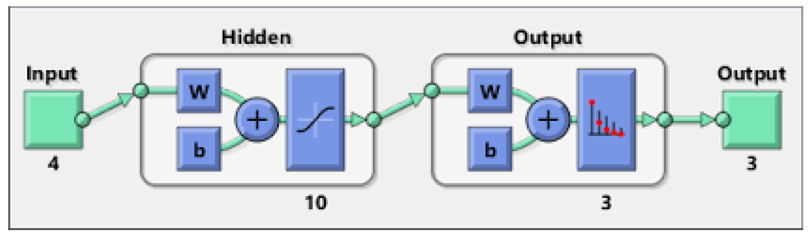
3.1. Multilayer Perceptron (MLP) Classifier

MLP is an type of ANN (Artificial Neural Network) composing thee layers: input, output and hidden. The number of the hidden layers depends on applications as well as the designer of this ANN. Each node in MLP classifier executes two functions. The first function calculates the weighted sum of the input (P) along with the bias ($\theta$) [20].

$$B_k=\sum _{i=1}^m\left(W_{ik}{P}_i\right)-{\theta }_{k}k=a,a_1,a_2,\dots ,m$$

(1)

where $P_i$ indicates to the input layer, $W_{ik}$ denotes to the relation weight from input layer i to jth hidden layers, ${\theta }_k$ indicates the bias of kth hidden layers and m is the number of input layer (neurons).

The second function, called activated function, is used to produce the output for each neuron, i.e.,

$$B_k=f\left(b_k\right)$$

(2)

$$f\left(b_k\right)=sigmoid\left(b_k\right)$$

(3)

$$sigmoid\left(b_k\right)=1/1+exp(-b_k)k=a,a_1,a_2,\dots ,m$$

(4)

Then the output layer is calculated using the following equation:

$$o_l=\sum _{k=1}^m\left(W_{kl}{B}_k\right)-\tilde{\theta }l=a,a_1,a_2,\dots ,m$$

(5)

where $W_{kl}$ denotes the relation weight from kth hidden layer to l output layer, $B_k$ is the bias of lth hidden layer and l is the output neuron. In the output layer, an activated function is used to produce the output layer for each neuron.

To train the optimal values of MLP, the weights and bias are required for desirable output. Figure 3 gives a schematic explanation for MLP model.

3.2. Extreme Learning Machine (ELM) Classifier

ELM is a Single Hidden Layer Feed Forward Neural Networks (SHLFNNs) learning algorithm. It works as follows: It randomly specifies the input weights and hidden layer biases and then analytically tests the output weights of SHLFNNs. ELM can achieve better performance than the other traditional learning algorithms in terms of fast learning speed. Also, ELM is less susceptible to user-specified parameters and can be deployed faster and more appropriately [21]. ELM can be expressed using the following equations. For S distinct samples with arbitrary ($y_k$, $u_k$), where $y_k={[y_{k1},y_{k2},\dots ,y_{km}]}^T\in R^m$ and $u_k={[u_{k1},u_{k2},\dots ,u_{kn}]}^T\in R^n$ the standard SHLFNNs with the number of hidden nodes L and activation function $f\left(y\right)$ are mathematically modeled as

$$\sum _{j=1}^L{\beta }_j{f}_j\left(Y_k\right)=\sum _{j=1}^L{\beta }_{j}f(W_j·Y_k+b_j)=O_{j}k=1,2,\dots ,S$$

(6)

where $w_j={[w_{j1},w_{j2},\dots ,w_{jm}]}^T$ is the weight vector linking the jth hidden node and the input nodes, ${\beta }_j={[{\beta }_{j1},{\beta }_{j2},\dots ,{\beta }_{jn}]}^T$ is the weight vector linking the jth hidden node and the output nodes, $b_j$ is the threshold of the jth hidden node, and $O_i={[O_{j1},O_{j2},\dots ,O_{jn}]}^T$ is the jth output vector of the SHLFNNs [21].

Given L hidden nodes and activation function $f\left(y\right)$, the SHLFNNs can approximate these S samples with zero error [21]. This can be modelled using the following equations:

$$\sum _{k=1}^L\parallel O_k-u_k\parallel =0$$

(7)

and there are ${\beta }_j$, $w_j$ and $b_j$ such that

$$\sum _{j=1}^L{\beta }_{j}f(W_j·Y_k+u_k)=u_{k}k=1,2,\dots ,S$$

(8)

Then

$$H\beta =T$$

(9)

where

$$H(w_1,w_2,\dots ,w_L,b_1,b_2,\dots ,b_L,y_1,y_2,\dots ,y_L)={\left[\begin{array}{cccc}f(w_1·y_1+b_1)& f(w_2·y_1+b_2)& \dots & f(w_L·y_1+b_L)\\ f(w_1·y_2+b_1)& f(w_2·y_2+b_2)& \dots & f(w_L·y_2+b_L)\\ .& .& .& .\\ .& .& .& .\\ f(w_1·y_S+b_1)& f(w_2·y_S+b_2)& \dots & f(w_L·y_S+b_L)\end{array}\right]}_{S\times L}$$

(10)

$$\beta ={\left[\begin{array}{cccc}{\beta }_{11}& {\beta }_{12}& \dots & {\beta }_{1n}\\ {\beta }_{21}& {\beta }_{22}& \dots & {\beta }_{2n}\\ .& .& .& .\\ .& .& .& .\\ {\beta }_{L1}& {\beta }_{L2}& \dots & {\beta }_{Ln}\end{array}\right]}_{L\times n}T={\left[\begin{array}{cccc}{T}_{11}& T_{12}& \dots & T_{1n}\\ T_{21}& T_{22}& \dots & T_{2n}\\ .& .& .& .\\ .& .& .& .\\ T_{S1}& T_{S2}& \dots & T_{Sn}\end{array}\right]}_{S\times n}$$

(11)

where H is the output matrix of the neural network, the jth column of H refers to the jth hidden node output given the inputs $y_1,y_2,\dots ,y_S$. From the solution of the above linear-system, the smallest norm least squares $\tilde{\beta }$ can be obtained by the following equation:

$$\tilde{\beta }=H†T$$

(12)

where $H†$ is known as the Moore–Penrose generalized inverse of the matrix H. Thus, the output function of ELM can be expressed as

$$g\left(y\right)=h\left(y\right)\beta =h\left(y\right)H†T$$

(13)

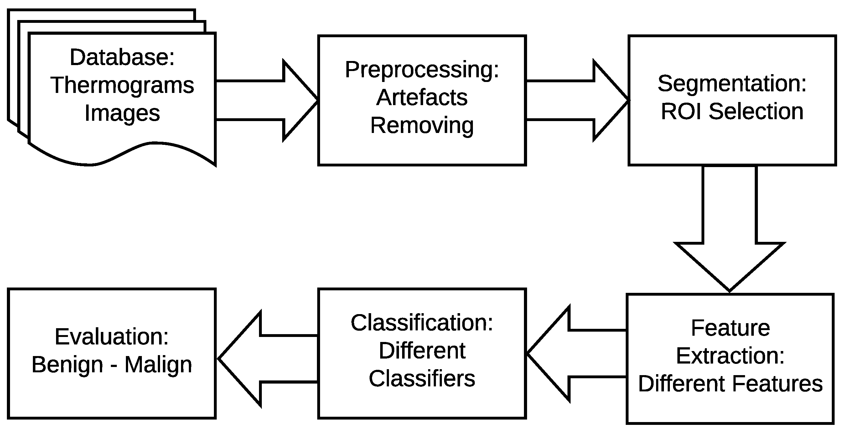
4. The Proposed Method

As shown in Figure 2 earlier, there are four main stages of a typical breast cancer detection system using digital thermography: (a) image preprocessing including artifact removing, (b) segmentation (extracting Region of Interest (ROI)), (c) feature extraction (i.e. extracting different features representing each sample), and (d) breast tumor detection (i.e. classifying each sample to either normal or abnormal). In the proposed method, these phases are summarized as follows (more details are given in Section 4.1, Section 4.2, Section 4.3 and Section 4.4):

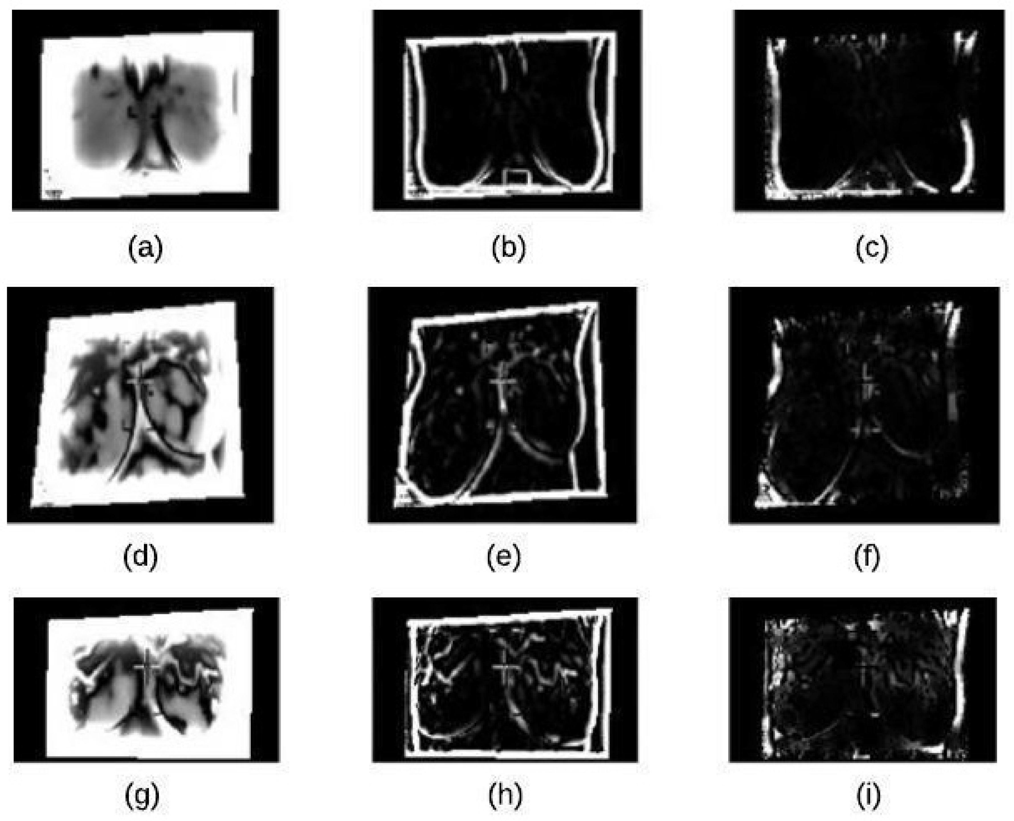
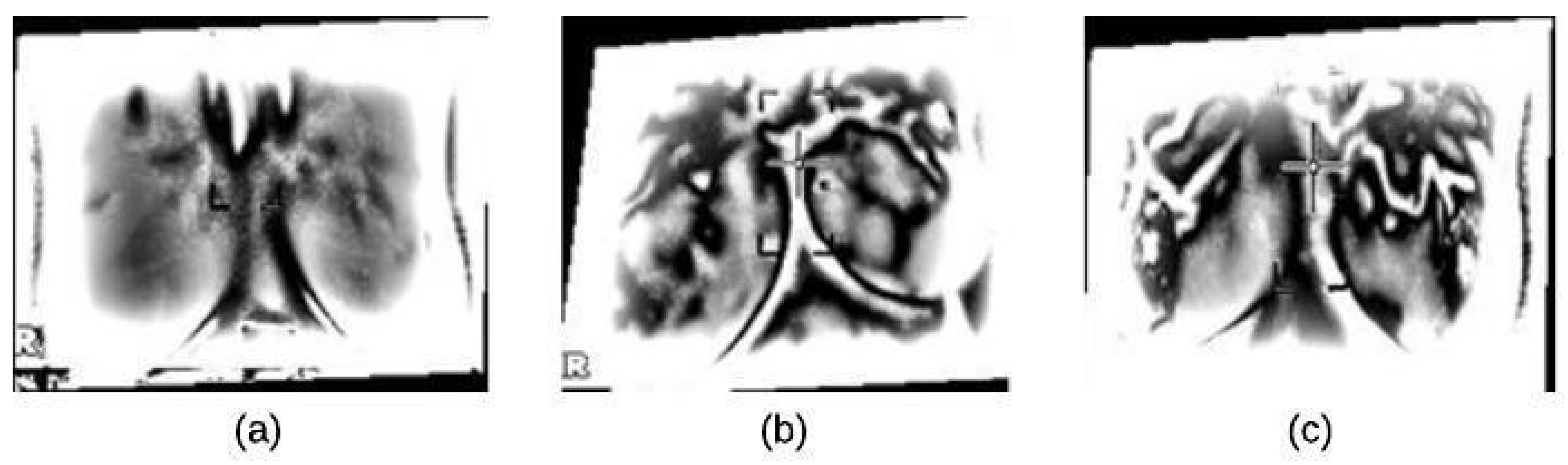
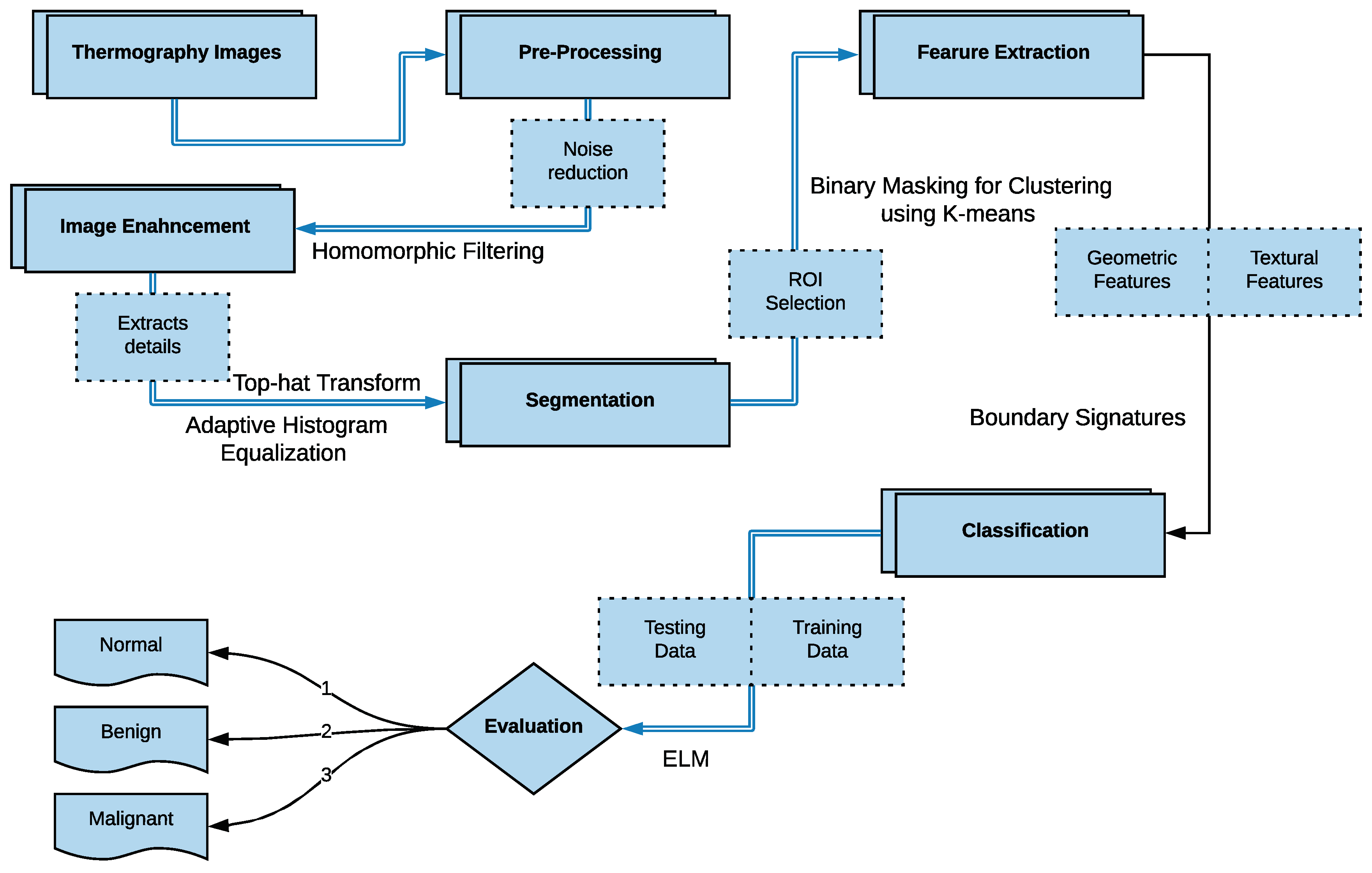
• In the image pre-processing stage: Noise reduction was achieved using the combination of homomorphic filtering and spatial domain morphology and image enhancement was accomplished using top-hat transform and adaptive histogram equalization.
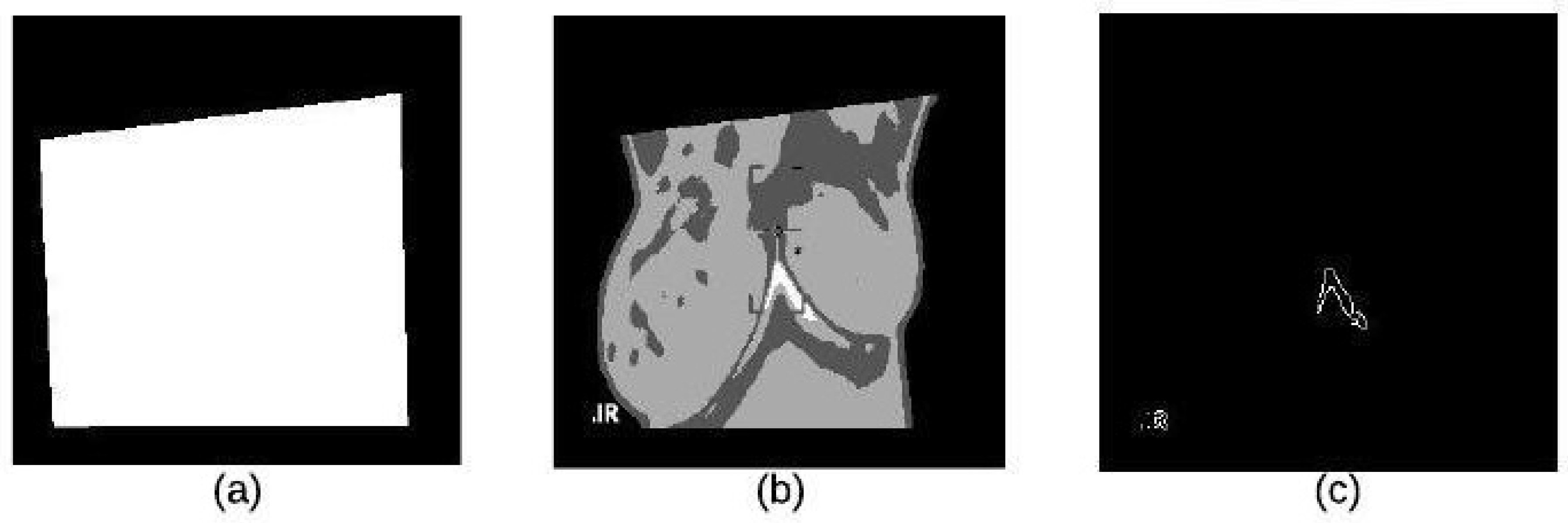
• In the segmentation stage, the tumor was segmented using binary masking and K-means clustering to produce the boundary image.
• In the feature extraction stage, two types of features were extracted: geometrical and textural features.
• In the tumor detection stage, MLP and ELM classifiers were used and compared.

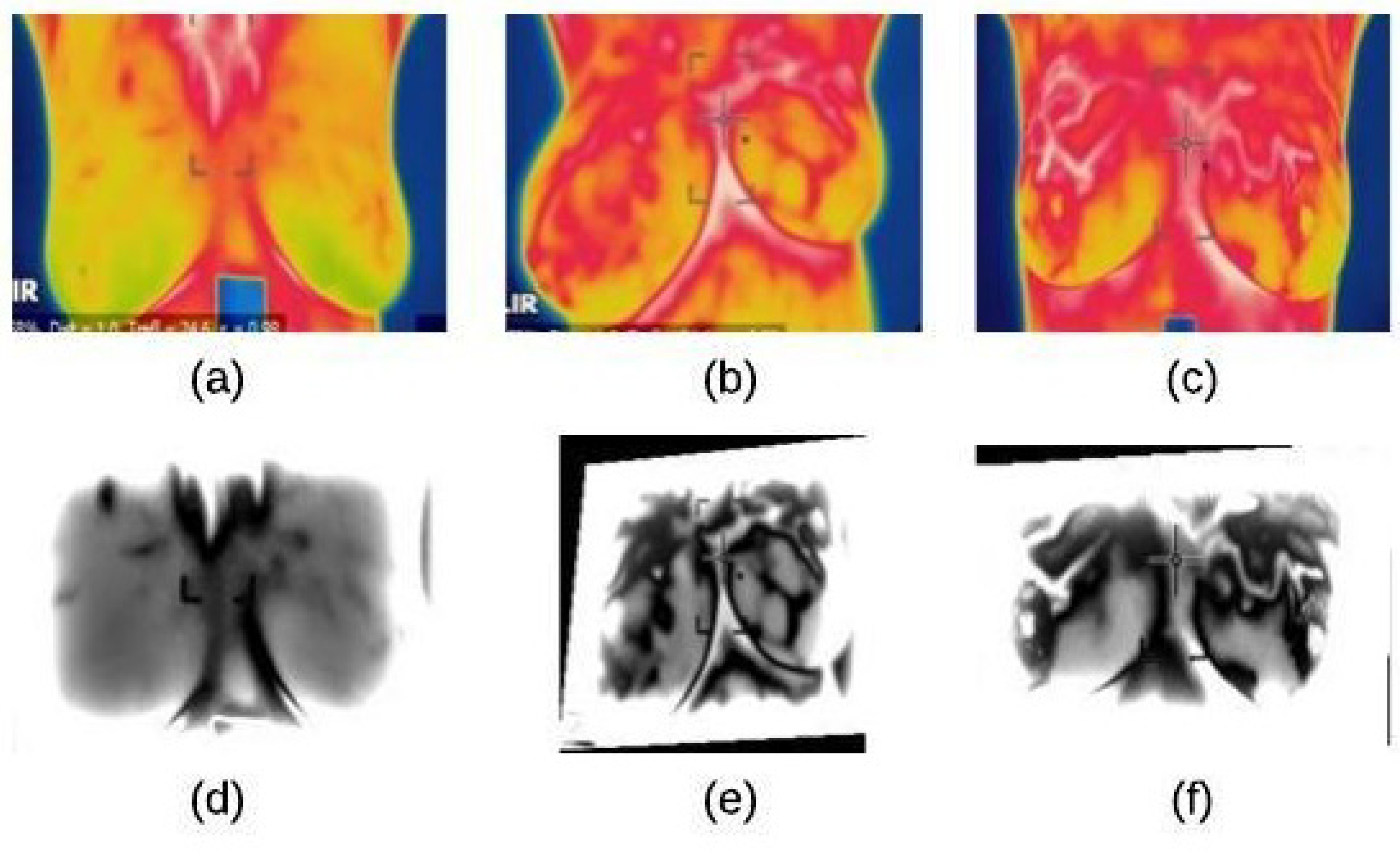
4.1. Image Preprocessing Stage

In this stage, two main processes have done: noise reduction and image enhancement.

4.1.1. Noise Reduction

The noise reduction process is achieve using a homomorphic filtering technique. This technique is applied to (1) remove multiplicative noise and (2) to improve the appearance intensity range illumination. As demonstrated in Algorithm 1, the homomorphic filtering firstly applies linear techniques to map the input image to a different domain and then mapping back the output to the original image domain. Also, it involves morphological operations to delete any noise and smooth the image’s edges [22]. The results of applying this technique and morphological operations are shown in Figure 4.

Algorithm 1 A homomorphic filtering technique

1: Read original thermal image, img 2: The image $img(v,w)$ is first converted into logarithm domain using the following equation: $$ln\left(img\right(v,w\left)\right)=ln\left(j\right(v,w\left)\right)+ln\left(f\right(v,w\left)\right)$$ 3: The output image is filtered by high-pass filter using Fast Fourier Transformation (FFT) using the following equation $$F(y,z)=F\left(ln\right(l(v,w)\left)\right)+F\left(ln\right(f(v,w)\left)\right)$$ where reflectance (f) and illumination (l) components. 4: The output image is filtered again using transfer function of frequency domain filter using the following equation: $$H(y,z)=(f_H-f_L)[1-exp(p(B/B_0^2)]$$ where $r_H>1$ and $r_L<1$ are the regulation parameter to change high frequency and low frequency respectively, D is balance parameter and $D_0$ is harmonic coefficient. 5: Inverse FFT is applied on the output of frequency domain filter as given in this equation: $$\stackrel{`}{H}(v,w)=invF\left(H(y,z)\right)$$ 6: Exponential is applied to the output of inverse FFT using this equation: $$G(v,w)=exp(\stackrel{`}{H}(v,w))$$

4.1.2. Image Enhancement

The enhancement process was achieved using Algorithm 2 which is designed based on the ideas in [22].

Algorithm 2 The enhancement process

1: Read thermal image, G(v,w) 2: Tophat transform is applied to $G(v,w)$ to separate the objects. $$\mathrm{Let}\mathrm{toph}1\mathrm{is}\mathrm{the}\mathrm{output}$$ where the size and shape of the structuring element are selected based on the size and shape of the masses. 3: Dilation operator is to gradually enlarge the regions boundaries of foreground pixels to smooth the borders of the tophat transformed image. $$\mathrm{Let}\mathrm{toph}2\mathrm{is}\mathrm{the}\mathrm{output}$$ 4: Bot-hat transform is used to smooth the objects in the image [22]. $$\mathrm{Let}\mathrm{toph}3\mathrm{is}\mathrm{the}\mathrm{output}$$ 5: This image is combined using Image arithmetic addition and subtraction as shown in Figure 5. $$Enhanced=\left(G\right(v,w)+toph2)-\left(toph3\right)$$ 6: Adaptive histogram equalization (AHE) technique is then used to improve the contrast of images produced in Step 5.

AHE executed in Step 5 computes several histograms of an image. Each of them corresponding to a distinct section of the image, and it then uses these histograms to redistribute the lightness values of the image. Thus, it enhances the edges’ definitions for each region of an image. The results of this algorithm are summarized in Figure 6.

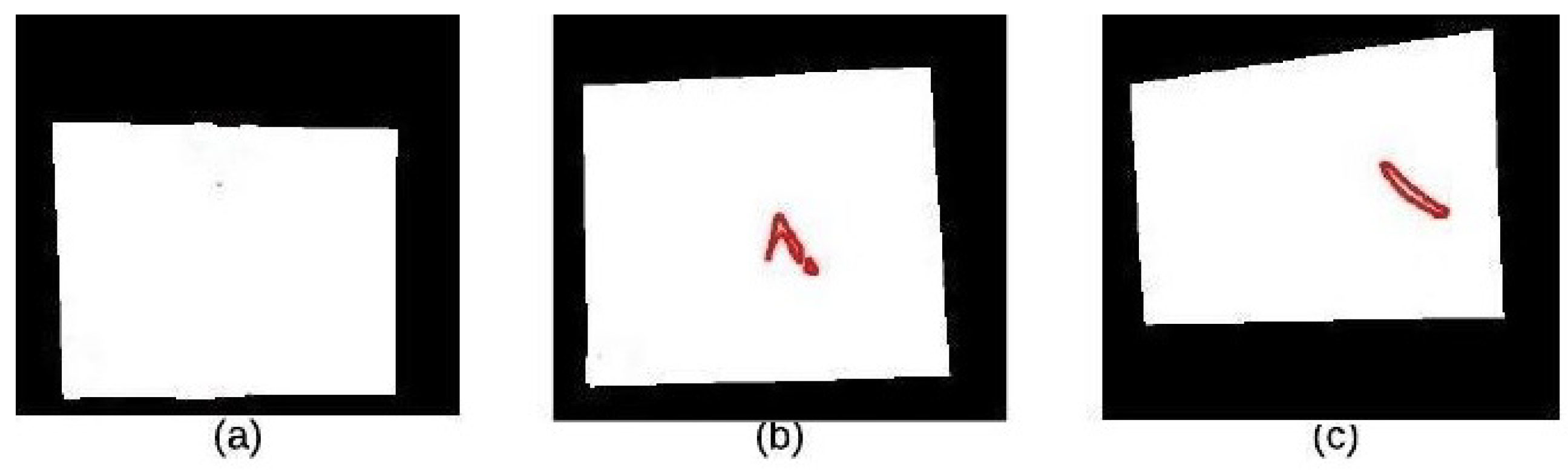
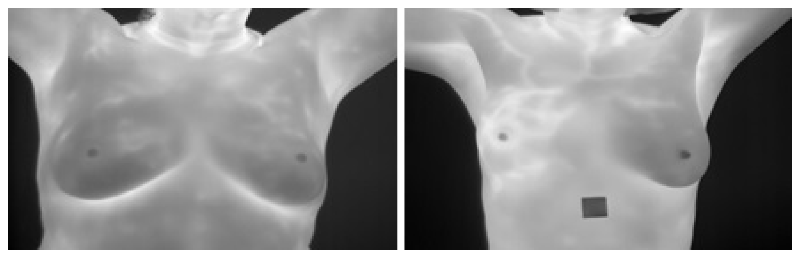
4.2. Segmentation Stage

The segmentation stage consists of three main steps which are based on the ideas in [22]: applying K-means clustering to extract the ROI, followed by binary morphology to remove small brights details and finally applying morphological gradient to remove the constant intensity areas and enhance edges. We summarize these stages as follows:

4.2.1. K-Means Clustering

K-mean clustering is used in our proposed method to divide thermal images into 3 clusters based on features to extract ROI. We considered the values of image pixels are grey-level. We have selected Euclidean distance as a distance measure to minimize the total of any pixel point to cluster centroid distances. The results of applying this k-means clustering technique and segmented mass are shown in Figure 7a–c.

4.2.2. Binary Morphology

To enhance thermal images, opening operations are utilized in our proposed method where they are used to remove small bright details in the image while leaving the overall pixel intensity values and large bright objects undisturbed. Mathematically, opening of image g with structuring element b is given by the following equation:

$$g\circ b=\left(g\theta b\right)\oplus b$$

(14)

4.2.3. Morphological Gradient

Erosion and dilation act as a local minimum and local maximum operator respectively. Image subtraction of these two operations gives a morphological gradient. This operation is used to enhance image edges by removing the constant intensity areas. The results, as illustrated in Figure 7c, show the boundary of the lesion. The morphological gradient is given by the following equation.

$$Morphological\left(Gradient\right)=Dilation\left(f\right)-Erosion\left(f\right)$$

(15)

4.3. Feature Extraction Stage

In this paper, we used the boundary signature-based features techniques [23] to extract features from thermogram images. A boundary signature is defined as a 1-D representation of this boundary. It can be seen as a plot of the distance from the boundary centroid to this boundary. Example of applying this technique to thermograms are shown in Figure 8a–c. They show the detected boundary of normal, benign mass and malignant mass. Figure 9a–c show the signatures of the detected boundaries.

4.3.1. Geometrical Feature Extraction

Based on the correlation between breast tumors and its locations and shapes, it is believed that geometrical features such as area, perimeter, P/A ratio, major axis, minor axis, LS ratio, and ENC are a very important for breast cancer detection. Below, we explain each geometrical feature which was used in the proposed method.

• Area: The total of all pixels (p) of the segmented nucleus (n).
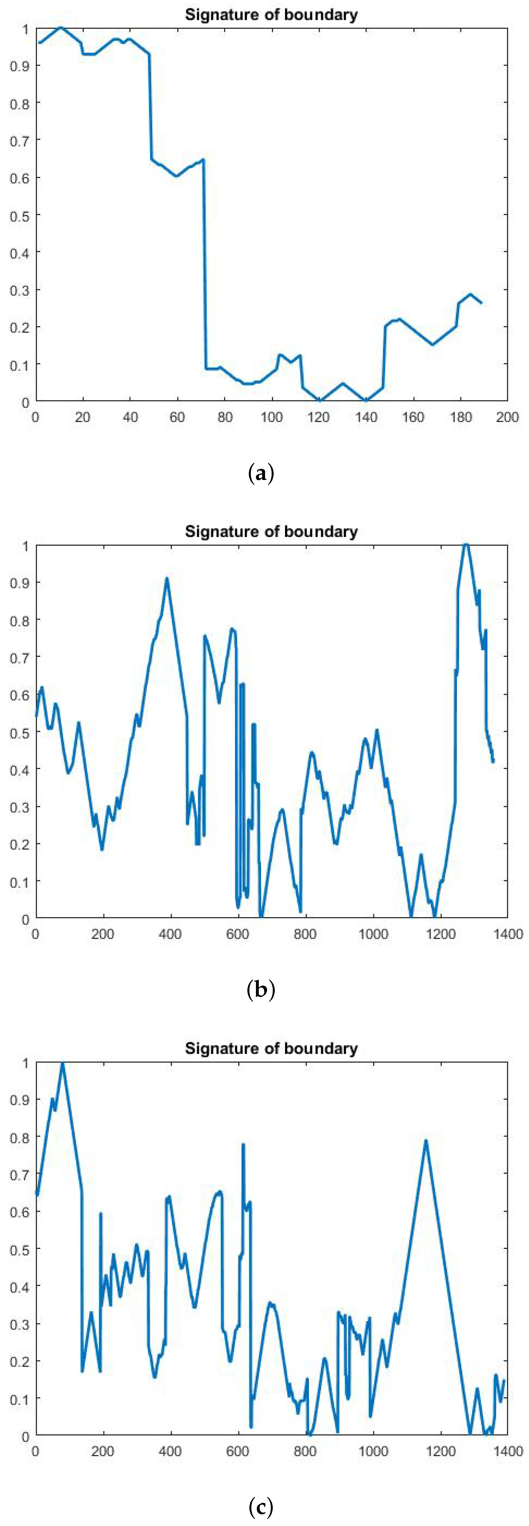
• Perimeter: The nuclear envelope length is computed as a polygonal length approximation of the boundary (B).
• P/A ratio: It is measured the degree to which the perimeter of the boundary (B) is exposed area ratio of the boundary (B).
• Major Axis Length (in pixels): It is computed as the length of the major axis of an ellipse having the same second moments as the region.
• Minor Axis Length (in pixels): It is computed as the length of the minor axis of an ellipse having the same second moments as the region.
• LS Ratio: It is computed as the length ratio of the major axis length to the minor axis length of the equivalent ellipse of the lesion.
• Elliptical normalized circumference(ENC): ENC features are computed in terms of the lesion circumference ratio and its equivalent ellipse.

4.3.2. Textural Feature Extraction

It is medically proved that the tumor distort a breast tissue. Thus, textural features become important in tumor detection. In recent years, there are many techniques for the extraction of textural features, e.g., GLCM (Gray Level Co-occurrence Matrix (GLCM) is a well-known texture features technique [24]. In the proposed method, the textural features extraction is used in the classification: entropy, EBCM, and standard deviation.

• Entropy: It is a statistical measure of randomness of an intensity image. It is used to represent the texture of a given image. Mathematically, an entropy of an image is computed as, $sum(H.\ast {\left(log\right)}_2\left(h\right))$, where h denotes the histogram counts for the intensity image [13].
• Edge-Based Contrast Measure (EBCM): This is a feature which depends on the human perception and is very sensitive to edges. Mathematically, EBCM feature of an image, I, is calculated as given in the following equation:

  $$EBCM=\sum _{h=1}^H\sum _{q=1}^Q(C(h,q)/hq)$$

  (16)

  $C(h,q)$ is a contrast value for an image pixel located at $(h,q)$ and is calculated as

  $$C(h,q)=\frac{\left|I\right(h,q)-e(h,q\left)\right|}{\left|I\right(h,q)+e(h,q\left)\right|}$$

  (17)

  where the mean gray level is:

  $$e(h,q)=\frac{{\sum }_{\left(\right(k,l\left)N\right(h,q\left)\right)}g(k,l)I(k,l)}{{\sum }_{\left(\right(k,l\left)N\right(h,q\left)\right)}g(k,l)}$$

  (18)

  where $N(h,q)$ is set of all neighboring pixels with the center pixel at $(p,q)$ and $g(k,l)$ is the edge value which is the image gradient magnitude. For EBCM, if EBCM value of output image is greater than the original image, it indicates the better contrast of output image.
• Standard Deviation: The standard deviation of gray-scale values, $\sigma$ is the estimate of the mean square deviation of the grey pixel value $v(x,y)$ from its mean volume. It describes dispersion within a local region. It is calculated using the formula

  $$\sigma =\sqrt{\frac{1}{MN}\sum _{(x=1)}^M\sum _{(y=1)}^N{(v(x,y)-\mu )}^2}$$

  (19)

4.4. Classification Stage

Classification is the last stage in the breast cancer detection technique which includes two operations: training and testing. The extracted features are given inputs into the classification techniques to evaluate whether an given thermogram is normal, benign tumor, or malignant tumor. In this paper, two classification techniques (i.e., MLP and ELM) are applied to evaluate the performance and accuracy of the proposed method.

In the MLP and ELM networks, the selection of the activation functions plays a substantial role in the performance of the network. Many studies have investigated special activation functions to solve different problems. So, in this paper, we investigated different activation functions in both MLP and ELM networks to evaluate which would give high accuracy and performance. The tested activation functions are: neuronal, sigmoid, logarithmic, hyperbolic tangent, exponential, and sinusoidal. The performances of the MLP and ELM networks are calculated based on the correct classification percentage. Figure 10 summarizes the proposed method.

5. Experiments

5.1. Dataset Description and Experiments Setup

The dataset used in the evaluation of the proposed method is DMR-IR database [25]. It consists of thermogram images and it is made available for researchers to evaluate their thermogram-based breast cancer detection proposals. Ii contains 1345 images: 705 normal, 200 benign tumors, and 440 malignant tumors. The patients are women between ages of 32 and 74 and thermal IR breast images are with size 640 × 480 pixels. All database images and their annotations are confirmed by radiologists. In the evaluation of the proposed method, 1000 samples of these images are utilized to train the proposed method and the remaining 345 samples are utilized to test and validate the proposed method. All experiments were conducted on a laptop/PC Core i5-2400 CPU 3.10 GHz with 4.00 GB. The implementation was compiled using MATLAB R2015a under Windows 10.

5.2. Experiments Scenarios

We designed several experimental scenarios to examine the best MLP and ELM activation functions and parameters giving the best results as well as the performance of MLP and ELM.

5.2.1. Scenario 1: MLP Activation Functions

The aim of this scenario is to investigate the best MLP activation functions. The best will be determined based on the highest classification accuracy obtained. The following MLP activation functions will be examined: saturating linear (satlin), linear (purelin), symmetric saturating linear (satlins), log-sigmoid (logsig), positive linear (poslin), and hyperbolic tangent sigmoid (tansig). In this scenario, the following steps were followed.

• The MLP number of layers was one for input, one hidden and one for the output.
• These layers were constant for each MLP activation function.
• The set of features were fixed for each MLP activation function.
• This experiment for each MLP activation function above.

5.2.2. Scenario 2: Training Time of MLP Activation Functions

This scenario is designed to understand the required training time for each MLP activation function during the classification process. In this scenario, the following steps were followed.

• The MLP number of layers was one for input, one hidden and one for the output)
• These layers were constant for each MLP activation function.
• The set of features were fixed for each MLP activation function.
• This experiment for each MLP activation function above
• The CPU time consumed was computed o get the final classification accuracy each MLP activation function.

5.2.3. Scenario 3: Numbers of Layers and Neurons per Each Hidden Layer of the Best MLP Activation Function

The aim of this scenario is to further investigate the best MLP activation functions (obtained from Scenario 1). For the best MLP activation, we aim to test which parameters would give the highest classification rate. Specifically, we will investigate the Numbers of layers and neurons for each hidden layer. In this scenario, the following steps were followed.

• We have tested the following parameters for the used neural network:

  (a)

  3 hidden layers and a number of neurons 4,5 and 10 respectively,

  (b)

  5 hidden layers and a number of neurons 4, 5 and 10 respectively and

  (c)

  7 hidden layers and a number of neurons 4, 5 and 10 respectively.

• For each of the above setup, a set of features were fixed for each experiment with the same chosen MLP activation function.
• the CPU time consumed was computed to get the final classification accuracy for each (1.a, 1.b, 1.c)

5.2.4. Scenario 4: Learning Rate of the Best MLP Activation Function

The aim of this scenario is to understand the impact of the learning rate of the best MLP activation functions (obtained from Scenario 1). We aim to test which value of the learning rate would give the highest classification rate. Specifically, we will investigate the effect of the numbers of hidden layers and their chosen neurons on the classification results. In this scenario, the following steps were followed.

• We have tested the following parameters for the used neural network:

  (a)

  3 hidden layers using number of neurons of 4, 5 and 10 respectively.

  (b)

  5 hidden layers using number of neurons of 4, 5 and 10 respectively.

  (c)

  7 hidden layers using number of neurons of 4, 5 and 10 respectively.

• For each of the above setup, learning rate $\eta$= 1, 3, 5, 7, 9 was tested and the obtained results were recorded.
• For each of the above setup, the set of features were fixed for each experiment with the same chosen MLP activation function.
• The CPU time consumed was computed to get the final classification accuracy for each value of $\eta$ set in Step 2.

5.2.5. Scenario 5: ELM Activation Functions

The aim of this scenario is to investigate the best ELM activation functions. The best will be determined based on the highest classification accuracy obtained. The following ELM activation functions will be examined: Sigmoid (sigmoid), Sine (sin), Triangular basis function (tribas), Hard Limit (hardlim), and Radial basis function (radbas). In this scenario, the following configurations were used.

• Three layers of ELM were used: one for input, one hidden and one for the output.
• These layers were constant for each ELM activation function.
• The set of features were fixed for each ELM activation function.
• This experiment was repeated for each ELM activation function above.

5.2.6. Scenario 6: Training Time of ELM Activation Functions

This scenario is designed to understand the required training time for each ELM activation function during the classification process. In this scenario, the following steps were followed.

• Three layers of ELM were used: one for input, one hidden and one for the output)
• These layers were constant for each ELM activation function.
• The set of features were fixed for each ELM activation function.
• This experiment was repeated for each ELM activation function above
• The CPU time consumed was computed to get the final classification accuracy each ELM activation function.

6. Results and Discussions

In this section, the results of the experiments run under all the scenarios above will be reported and discussed. It will first present MLP results and then the ELM ones. The reported results of the accuracy, specificity and sensitivity are the average of ten runs of the proposed method.

6.1. The Results of Scenario 1

The accuracy of training and testing of the different activation functions are compared. All results of the activation functions are presented in

Table 1. The results of Scenario 1: MLP Activation Functions.

Activation Functions	Accuracy
tansig	0.7424
logistic	0.6996
poslin	0.615
satlins	0.6076
satlin	0.6142
purlin	0.6466

. The best results (accuracy of the trained and tested data) were obtained using the “tansig” activation function. This best function (tansig) was then further evaluated in terms of specificity, sensitivity, the results 84% for specificity and 61.6% for sensitivity.

6.2. The Results of Scenario 2

The time required for training of the different activation functions are compared. All results of activation functions are presented in

Table 2. The results of Scenario 2: MLP Training Time.

Activation Functions	Training Time
tansig	3.086165
logistic	3.473274
poslin	3.182216
satlins	3.047807
satlin	2.957490
purlin	2.890241

. The best results of the training time were obtained using the “purlin” activation function and it was 2.890241 s. Although this time is better than tansig’s time but it is quite a small amount (0.195924 s). The current advance in computer speed (supercomputer and GPU) would make this processing time irrelevant.

6.3. The Results of Scenario 3

The accuracy of training and testing of different number of layers and neurons used for each hidden layer of “tansig” activation function are compared. All results of accuracy are presented in

Table 3. The results of Scenario 3: The accuracy and training time for different configurations of “tansig” activation function.

No. of Layers	Neurons = 4		Neurons = 10		Neurons = 5
	Accuracy	Time	Accuracy	Time	Accuracy	Time
3	0.6892	3.29759 s	0.7834	5.615519 s	0.7010	3.416063 s
5	0.6684	4.014458 s	0.8042	10.3971355 s	0.6788	4.145014 s
7	0.6958	3.838878 s	0.8220	15.811615 s	0.7025	5.98080 s

. From this table, it can be noticed that the best result (accuracy at 82.20% with training time 15.811615s) was obtained when the number of hidden layers and neurons were 7 and 10 respectively

The results of this scenario showed a positive relationship between the training time and the number of neurons. The training time increases when the number of neurons increases. From Table 3, we found that when the number of neurons was 10, the training times increased. Similarly, the results showed a positive relationship between the training time and the accuracy of training. The accuracy of training increases if the training time increases. From Table 3, the accuracy of training was the best result when the training times increased.

6.4. The Results of Scenario 4

Based on the results given in scenario 1, the activation function “tansig” was further tested with different learning rates and compared when the number of hidden layers was 7 and the number of neurons was 10. All results of accuracy are presented in

Table 4. The results of Scenario 4: The accuracy and training time of different learning rate for the “tansig” activation function.

Learning Rate	Accuracy	Training Time
1	0.8004	17.687415 s
3	0.7730	13.623254 s
5	0.7886	13.707897 s
7	0.7834	13.646803 s
9	0.7864	13.244280 s

. The best results of the accuracy were obtained using the “tansig” activation function, the learning rate was 1.00 and accuracy was 80.04% with training time was 17.687415 s.

6.5. The Results of Scenario 5

The accuracy of training and testing of the different activation functions are evaluated and compared. The summary of the results of this scenario is presented in

Table 5. The results of Scenario 5: ELM Activation Functions.

Activation Function	Accuracy
sigmoid	0.9887
sin	0.9901
hardlim	0.8902
tribas	0.9910
radbas	0.9889

. The best results (accuracy of the trained and tested data) were obtained using the “tribas” activation function and it was 99.10%. In general, from Table 1 and Table 5, it can be noticed that the ELM classifier’s accuracy results are much better than MLP classifier’s ones.

6.6. The Results of Scenario 6

All results of training time of different activation functions are presented in

Table 6. The results of Scenario 6: ELM Activation Functions.

Activation Function	Training Time
sigmoid	0.0469
sin	0.0035
hardlim	0.0625
tribas	0.0015
radbas	0.0050

. The best result was obtained during the training time using the “tribas” activation function and it was 0.0015 s. In general, from Table 2 and Table 6, it can be noticed that ELM classifier needed less time than MLP classifier. This logic as ELM only has one hidden layer while MLP needs 7 hidden layers to produce the best results.

To compare our results with the most related work, we conducted a comparison and its results are summarized in

Table 7. The comparison between the proposed work and the other related work.

Paper/Criteria	Dataset Size	Public/Private Dataset	Classifiers	Accuracy	Specificity	Sensitivity
A. Kennedy [2009]	−	Private	TH(1:5)scale	−	−	95%
Pramanik [2016]	40 malignant 60 benign	Public(DMR)	FANN	90%	85%	95%
Rafal [2016]	325 examin.	Private	Naive Bayes Decision Tree	−	−	−
			SVM R. Forrest
Acharya [2010]	40 normal 60 malignant	Private	SVM	88.10%	90.48%	85.71%
Gaber [2015]	29 healthy 34 malignant	Public(benchmark)	SVM	92.06%	−	−
Gogo [2018]	70 abnormal 50 normal	Private	SVM(Poly)	98%	98%	98%
Sathish [2018]	−	Public (DMR)	E. Bagg. Trees AdaBoost	87%	90.6%	83%
Our Solution	705 normal 200 benign 440 malignant	Public (DMR-IR)	MLP ELM	80.04% 99.10%	84% 98.05%	61.6% 97.03%

. From this table, it can be noticed that the results obtained by ELM algorithm is the best in terms of the accuracy, specificity, and sensitivity. In addition, our results have obtained from the largest dataset of all the compared work. This means that our results would be much reliable in terms of the scale-ability.

In addition to the above comparison, we compared our method with the CNN based method [26] which reported classification results (TPR = 100% and PPV = 100% using a dataset containing 73 breast images). It is obvious that the CNN-based method achieved a slightly better results. However, our results are concluded from using a large dataset (1345 images) while CNN-based one obtained from 73 breast images.

7. Conclusions

This paper introduced a comparative study between two machine learning techniques (MLP and ELM) for the early detection of breast cancer through thermograms. Before applying any of these techniques, the entered images were firstly pre-processed, ROI was then segmented and finally, features were extracted. Under different scenarios, experiments were conducted using public dataset (DMR-IR). Different activation functions of both MLP and ELM were tested and investigated too. The experimental results showed that ELM-based breast cancer detection gave the best accuracy (100%) while the MLP classifiers gave only 82.20%. The ELM results were obtained using its TRIBAS function and only one hidden layer. Also, it was found that ELM is much faster than MLP. These promising detection results would be an important step toward an automatic detection of breast cancer using thermal images. The limitation of the proposed method depends on the quality of the protocol used to capture the thermograms. As the thermal images depends mainly on the temperature, the room and patient’s temperature could affect the predication techniques. In future work, we think there are two points which could further improve/confirm the results of this study. Firstly, a thorough comparison and analysis between ELM and CNN could be conduct. Secondly, to advance the performance of the proposed segmentation technique, it is suggested to use more extracted features of different types to evaluate the classifier performance.

References

1. Gaber, T.; Ismail, G.; Anter, A.; Soliman, M.; Ali, M.; Semary, N.; Hassanien, A.E.; Snasel, V. Thermogram breast cancer prediction approach based on Neutrosophic sets and fuzzy c-means algorithm. In Proceedings of the 2015 37th Annual International Conference of the IEEE Engineering in Medicine and Biology Society (EMBC), Milan, Italy, 25–29 August 2015; pp. 4254–4257. [Google Scholar]
2. Sickles, E.A. Mammographic Features of early Breast Cancer. Am. J. Roentgenol. 1984, 143, 461–464. [Google Scholar] [CrossRef] [PubMed]
3. Nover, A.B.; Jagtap, S.; Anjum, W.; Yegingil, H.; Shih, W.Y.; Shih, W.H.; Brooks, A.D. Modern Breast Cancer Detection: A technological Review. J. Biomed. Imaging 2009. [Google Scholar] [CrossRef] [PubMed]
4. Lee, H.; Chen, Y.P.P. Image Based Computer Aided Diagnosis System for Cancer Detection. Expert Syst. Appl. 2015, 42, 5356–5365. [Google Scholar] [CrossRef]
5. Etehad Tavakol, M.; Chandran, V.; Ng EKafieh, R. Breast Cancer Detection from Thermal Images Using Bispectral Invariant Features. Int. J. Therm. Sci. 2013, 69, 21–36. [Google Scholar] [CrossRef]
6. Tan, T.Z.; Quek, C.; Ng, G.; Ng, E. A novel Cognitive Interpretation of Breast Cancer Thermography with Complementary Learning Fuzzy Neural Memory Structure. Expert Syst. Appl. 2007, 33, 652–666. [Google Scholar] [CrossRef]
7. Arakeri, M.P.; Reddy, G.R. Computer-Aided Diagnosis System for Tissue Characterization of Brain Tumor on Magnetic Resonance images. SIViP 2015, 9, 409–425. [Google Scholar] [CrossRef]
8. Etehadtavakol, M.; Ng, E.Y. Breast Thermography as A potential Non-Contact Method in the Early Detection of Cancer: A review. J. Mech. Med. Biol. 2013, 13, 1330001. [Google Scholar] [CrossRef]
9. Sathish, D.; Kamath, S.; Rajagopal, K.V.; Prasad, K. Medical Imaging Techniques and Computer Aided Diagnosis Approaches for the Detection of Breast Cancer with an Emphasis on Thermography A review. Int. J. Med. Eng. Inform. 2016, 8, 275–299. [Google Scholar] [CrossRef]
10. Ali, M.A.; Sayed, G.I.; Gaber, T.; Hassanien, A.E.; Snasel, V.; Silva, L.F. Detection of breast abnormalities of thermograms based on a new segmentation method. In Proceedings of the 2015 Federated Conference on Computer Science and Information Systems (FedCSIS), Lodz, Poland, 13–16 September 2015; pp. 255–261. [Google Scholar]
11. Lipari, C.A.; Head, J. Advanced Infrared Image Processing for Breast Cancer Risk Assessment. In Proceedings of the 19th Annual International Conference of the IEEE Engineering in Medicine and Biology Society, Chicago, IL, USA, 30 October–2 November 1997; Volume 2, pp. 673–676. [Google Scholar]
12. Moghbel, M.; Mashohor, S. A review of Computer Assisted Detection/Diagnosis (CAD) in Breast Thermography for Breast Cancer Detection. Artif. Intell. Rev. 2013, 39, 305–313. [Google Scholar] [CrossRef]
13. Lee, M.Y.; Yang, C.S. Entropy-based feature extraction and decision tree induction for breast cancer diagnosis with standardized thermograph images. Comput. Methods Programs Biomed. 2010, 100, 269. [Google Scholar] [CrossRef] [PubMed]
14. Kennedy, D.A.; Lee, T.; Seely, D. A comparative review of thermography as a breast cancer screening technique. Integr. Cancer Ther. 2009, 8, 9–16. [Google Scholar] [CrossRef] [PubMed]
15. Pramanik, S.; Bhattacharjee, D.; Nasipuri, M. Texture analysis of breast thermogram for differentiation of malignant and benign breast. In Proceedings of the 2016 International Conference on Advances in Computing, Communications and Informatics (ICACCI), Jaipur, India, 21–24 September 2016; pp. 8–14. [Google Scholar]
16. Okuniewski, R.; Nowak, R.M.; Cichosz, P.; Jagodziński, D.; Matysiewicz, M.; Neumann, Ł.; Oleszkiewicz, W. Contour classification in thermographic images for detection of breast cancer. Proc. SPIE 2016. [Google Scholar] [CrossRef]
17. Acharya, U.R.; Ng, E.Y.K.; Tan, J.-H.; Sree, S.V. Thermography based breast cancer detection using texture features and support vector machine. J. Med. Syst. 2010, 36, 1503–1510. [Google Scholar] [CrossRef] [PubMed]
18. Gogoi, U.R.; Bhowmik, M.K.; Bhattacharjee, D.; Ghosh, A.K. Singular value based characterization and analysis of thermal patches for early breast abnormality detection. Australas. Phys. Eng. Sci. Med. 2018, 41, 861–879. [Google Scholar] [CrossRef] [PubMed]
19. Sathish, D.; Kamath, S. Detection of Breast Thermograms using Ensemble Classifiers. J. Telecommun. Electron. Comput. Eng. (JTEC) 2018, 10, 35–39. [Google Scholar]
20. Jadoon, M.; Zhang, Q.; Haq, I.U.; Jadoon, A.; Basit, A.; Butt, S. Classification of Mammograms for Breast Cancer Detection Based on Curvelet Transform and Multi-Layer Perceptron. Biomed. Res. 2017, 28, 4311–4315. [Google Scholar]
21. Wang, Z.; Yu, G.; Kang, Y.; Zhao, Y.; Qu, Q. Breast Tumor Detection in Digital Mammography Based on Extreme Learning Machine. Neuro Comput. 2014, 128, 175–184. [Google Scholar] [CrossRef]
22. Paramkusham, S.; Rao, K.M.; Rao, B.P. Automatic Detection of Breast Lesion Contour and Analysis using Fractals through Spectral Methods. In Proceedings of the International Conference on Advances in Computer Science, AETACS, National Capital Region, India, 13–14 December 2013. [Google Scholar]
23. Mencattini, A.; Salmeri, M.; Casti, P.; Raguso, G.; L’Abbate, S.; Chieppa, L.; Ancona, A.; Mangieri, F.; Pepe, M.L. Automatic breast masses boundary extraction in digital mammography using spatial fuzzy c-means clustering and active contour models. In Proceedings of the IEEE International Workshop on Medical Measurements and Applications Proceedings (MeMeA), Bari, Italy, 30–31 May 2011; pp. 632–637. [Google Scholar]
24. Bai, X.; Wang, K.; Wang, H. Research on the Classification of Wood Texture Based on Gray Kevel Co-occurrence Matrix. J. Harbin Inst. Technol. 2005, 37, 1667–1670. [Google Scholar]
25. Silva, L.F.; Saade, D.C.M.; Sequeiros, G.O.; Silva, A.C.; Paiva, A.C.; Bravo, R.S.; Conci, A. A new database for breast research with infrared image. J. Med. Imaging Health Inform. 2014, 4, 92–100. [Google Scholar] [CrossRef]
26. Tello-Mijares, S.; Woo, F.; Flores, F. Breast Cancer Identification via Thermography Image Segmentation with a Gradient Vector Flow and a Convolutional Neural Network. J. Healthc. Eng. 2019. [Google Scholar] [CrossRef] [PubMed] [Green Version]
Figure 1. Examples for Breast Thermograms Images: on the left a normal breast while on the right abnormal one.
Applsci 10 00551 g001
Figure 2. Typical breast cancer detection system.
Applsci 10 00551 g002
Figure 3. A typical MLP model.
Applsci 10 00551 g003
Figure 4. Homomorphic filtering result on thermographic images: (a) input image (normal) (b) input image (benign) (c) input image (malignant) (d) homomorphic filtering on normal image (e) homomorphic filtering on benign image (f) homomorphic filtering on malignant image.
Applsci 10 00551 g004
Figure 5. Top-hat Transform Technique: (a) homomorphic filtering on normal image (b) white top-hat on normal image (c) black top-hat on normal image (d) homomorphic filtering on benign image (e) white top-hat on benign image (f) black top-hat on benign image (g) homomorphic filtering on malignant image (h) white top-hat on malignant image (i) black top-hat on malignant image.
Applsci 10 00551 g005
Figure 6. Adaptive histogram equalization (AHE): (a) normal image (b) benign image (c) malignant image.
Applsci 10 00551 g006
Figure 7. K-means Clustering: (a) Binary Image (b) K-means Cluster Image (c) Boundary Image.
Applsci 10 00551 g007
Figure 8. Detected Boundary: (a) Normal (b) Benign mass (c) Malignant mass.
Applsci 10 00551 g008
Figure 9. (a) Normal image (b) Benign image (c) Malignant image.
Applsci 10 00551 g009
Figure 10. Flowchart of the Proposed Method.
Applsci 10 00551 g010