M-Shape PV Arrangement for Improving Solar Power Generation Efficiency

Abstract

This paper presents a novel design scheme to reshape the solar panel configuration and hence improve power generation efficiency via changing the traditional PVpanel arrangement. Compared to the standard PV arrangement, which is the S-shape, the proposed M-shape PV arrangement shows better performance advantages. The sky isotropic model was used to calculate the annual solar radiation of each azimuth and tilt angle for the six regions which have different latitudes in Asia—Thailand (Bangkok), China (Hong Kong), Japan (Naha), Korea (Jeju), China (Shenyang), and Mongolia (Darkhan). The optimal angle of the two types of design was found. It emerged that the optimal tilt angle of the M-shape tends to 0. The two types of design efficiencies were compared using Naha’s geographical location and sunshine conditions. Through economic analyses, both the photovoltaic base cost and the electricity sales revenue were calculated, and the results showed that the M-shape has better economic benefits compared to the S-shape design. The proposed method can save resources and improve economic efficiency as well.

1. Introduction

Global climate change is characterized by global warming and has huge repercussions on living things; as such, it is considered as one of the most serious challenges that humanity is facing in the 21st century. Emissions of greenhouse gases such as carbon dioxide are a cause of global warming [1]. The effects of nonrenewable energy in terms of economy, sufficiency, and sustainability are self-evident to humans. The growth in global renewable energy generation has increased drastically to 2351 GW as of 2019. Most of the renewable energy generation in 2018 was from wind and solar energy, with capacities of 564 and 486 GW, respectively. Renewable energy generation increased compared to the same period last year (171 GW or +7.9%). Solar energy continues to dominate, with capacity increasing by 94 GW (+24%), followed by 49 GW (+10%) of wind energy [2]. Due to its large storage capacity, being ubiquitous on earth and of an environmentally friendly nature, the utilization of solar energy has received much attention. The prices of PV systems have reduced considerably by 100% over the past 40 years from 76.67 per watt in 1977 to 0.74 per watt in 2013 [3]. Hence, solar energy is progressively entering the blowout period. Adjusting and optimizing the energy structure and systems is a necessity to protect the environment and increase power generation.

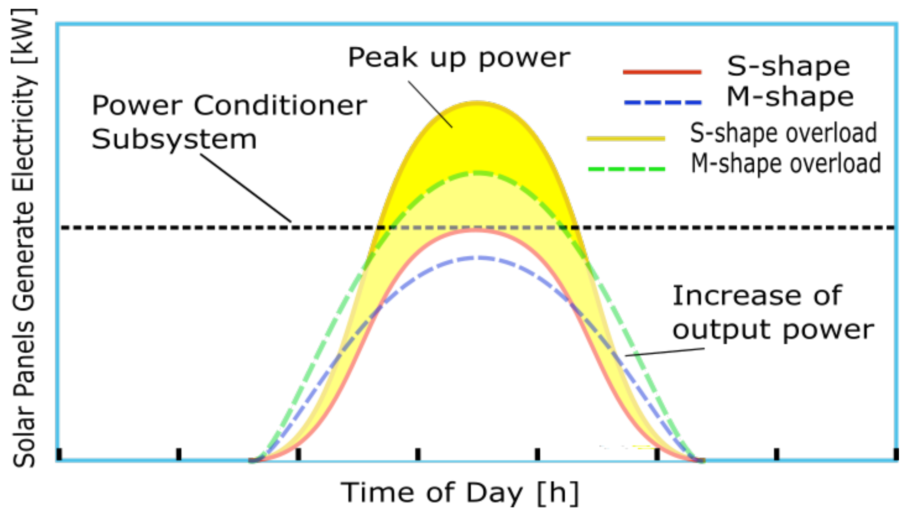
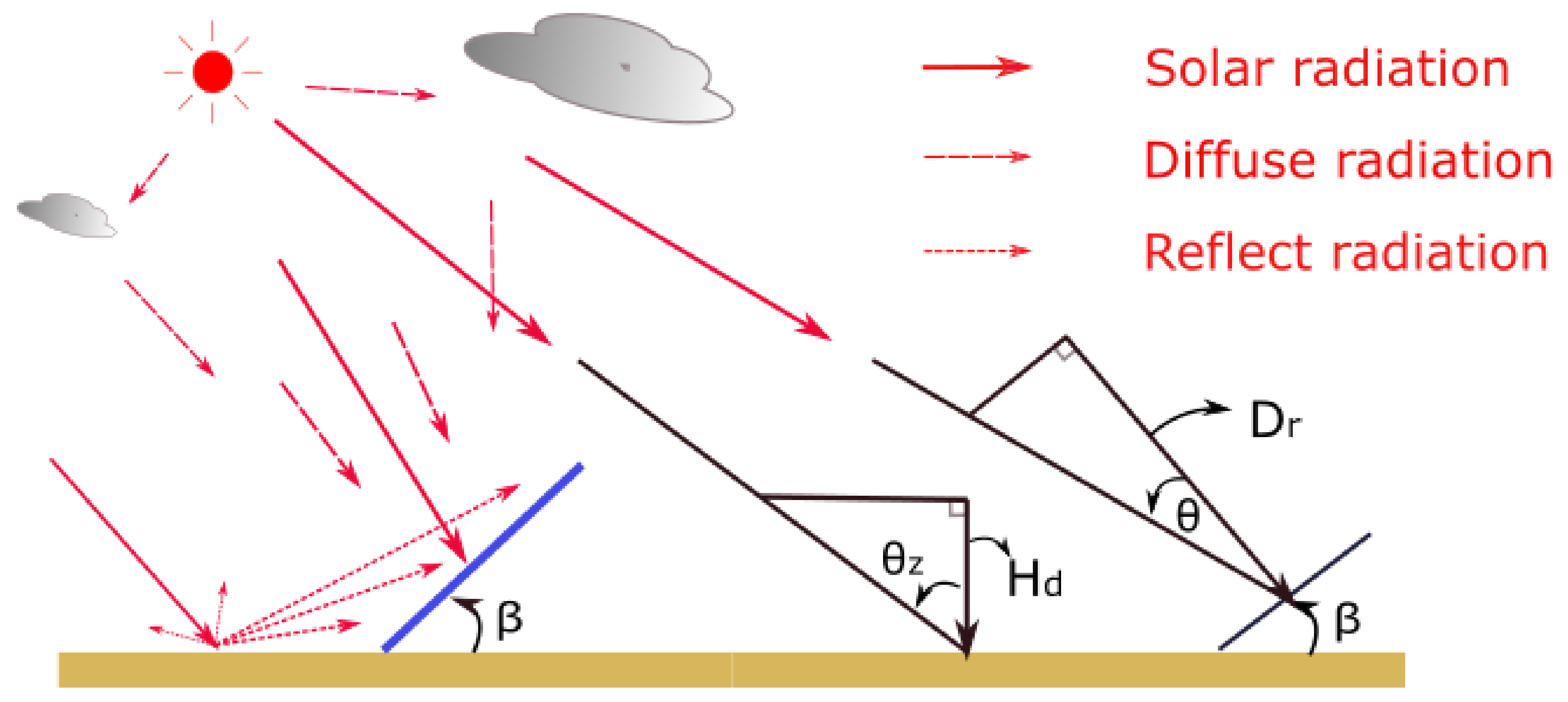
In the PV system, the power conditioning system (PCS) is important for solar energy facilities. Low-quality power will cause unnecessary damage to electrical equipment. PCSs are, however, relatively expensive, even though they play a major role in PV’s efficiency. Therefore, it is more important to make full use of PCSs. One of the solutions to making efficient use of them is to overload the PVs. Sometimes, due to cloudy days or winter reasons, overloading is also needed. Fiorelli et al. [4] discussed the advantage of PV system-to-PCS overload. Overloading is a condition whereby the PV panel that has been installed exceeds PCS capacity. Oversizing the PV array-to-inverter ratio can improve solar-power system performance by increasing the number of solar panels to ensure maximum energy harvest from each PV module in the system; this is coupled with power-limiting functionality. Power limiting is a PCS’s function that occurs when the available power from the PV arrays is greater than the PCS’s rated input power. Power limiting is often called “Clipping” or “Peak Cut” due to the flattening effect on the system’s daily production profile, as shown in Figure 1.

It can be seen from Figure 1 that the time when M-shape output power grows is in the morning and nightfall. Changing the PV design can increase the maximum output power, which could lead to very good research. Many studies have proposed different PV tree designs [5,6,7]. Dey et al. [5] proposed an optimization based on a genetic algorithm for the positioning of solar panels and obtained a scheme with less than 2% shadow loss. Hyder et al. [6] analyzed the power generation and ground efficiency. It was pointed out that in Kuala Lumpur, Bhopal, and Barcelona, the power generation efficiency percentage increase was 17.79%, 41.06%, and 20.97%, and land-use efficiency increased to 32.09%, 43.35%, and 33.87%, respectively. Verma et al. [7] created a complex 3D leaf-like PV arrangement which can collect more sunlight than traditional flat configurations. It is concluded that in winter, trees increased the amount of sunlight captured during daylight by 322%, while in summer, the improvement was 57%. In those designs, the structural characteristics of the simulated trees were used to improve the reception of sunlight. This can greatly save the floor space and when used as street light, it can enhance the viewing of the block. It also satisfies the current pressing social, cultural, and environmental PV system design requirements. However, there is no obvious advantage in terms of power generation efficiency. Alok et al. [8] wrote a review of the floating photovoltaic power plant. It was reported that the floating power plant is 11% more efficient than the land-sited PV system of a similar rating. Results showed that it is about 1.2% times higher than the conventional solar power plant in terms of the investment cost. There is another important reason. When photovoltaic cells are working, the shading of shadows has a great effect on them. Therefore, in practice, it is difficult to use the same distribution of panels as leaves. Bernardi et al. [9] demonstrated that absorbers and reflectors can be combined in the absence of sun-tracking to build three-dimensional photovoltaic structures that can generate measured energy densities which are higher by a factor of 2–20 than stationary flat PV panels. In fact, the M-shape is also a 3d structure. Kougias et al. [10] proposed an alternative method in which solar photovoltaic systems were installed on the available surfaces of existing water infrastructure (dams, irrigation canals) in the Mediterranean islands. This design creates a synergy between the energy-generating PV system and the water infrastructure. As we all know, for modern humans, water and energy are necessary things on the island. With the M-shape, it will save more space, which means that more panels can be set. Distributed photovoltaics (PV) is reported to roughly contribute 50% of the total globally installed solar energy capacity. Rooftop PV systems remain significant and give economic benefits [11]. Mukisa et al. 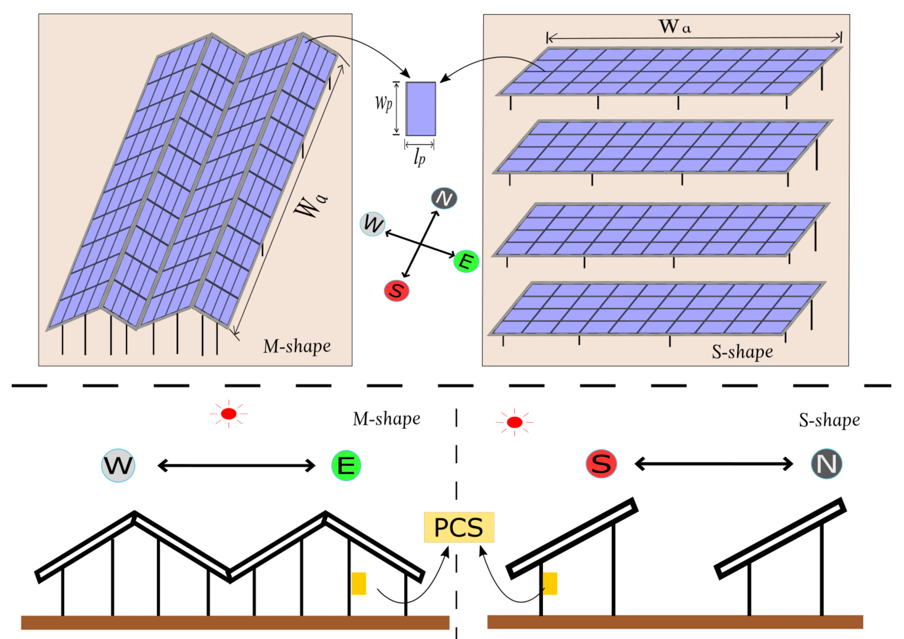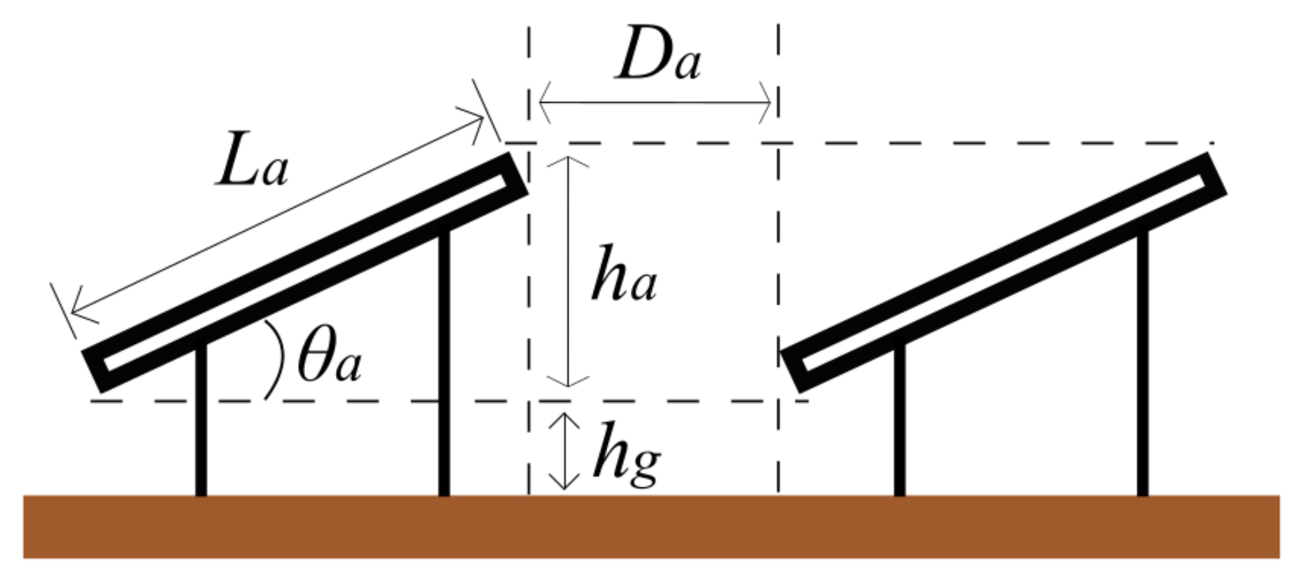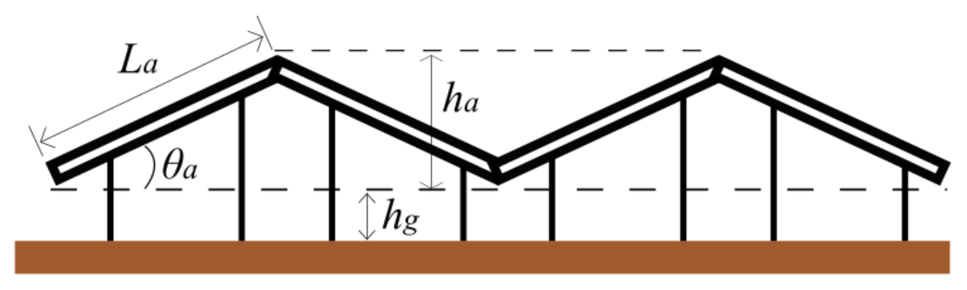[12] proposed a rooftop-estimating method. This approach does not require much equipment or tools and computer skills. Smart tracking solar panels are not good for rooftops, because there is not enough space to rotate. Firstly, it is more expensive for families. They require adjustment at any time, which makes them difficult to be deployed in small locations. Adjusting the placement of solar panels can, however, increase the number of panels, as this concept highly depends on the area of the rooftop. This will avoid peak power and lead to very good research. In addition, harsh environments are not suitable for smart panels. For example, PV panels fixed in typhoon-prone areas such as Okinawa will be more stable. Because of the fact that the M-shape PV panel design has a triangular shape, it is stronger. In view of this, this work sought to investigate the possibility of increasing the PV system power generation by changing the conventional PV array arrangement with solar panel azimuths towards the east and the west (M-shape). Simulations were performed in six cities in the Asia region with different latitudes. This design was reported to increase power generation by 15% by NTTin Japan [13], and details are shown in Figure 2.

Owing to the fact that the total energy of photovoltaic power is derived from the sun, the amount of solar radiation energy will be related to latitude, sunshine time, air quality, and geographic location. The power generation of photovoltaic panels is affected by the installation angle; hence, changing the natural environment is a bold idea, so that an optimal tilt angle is achieved to increase the amount of power generated. Studies [14,15] have provided references for calculating the optimal tilt angle, and the same method was used to find the best tilt angle by calculating the solar radiation model of the inclined plane. Yadav et al. [14] provided two types of methods to calculate the solar, isotropic, and anisotropic model. However, these approaches did not provide enough conviction in the study. There were still uncertainties with the approaches. Stanciu et al. [15] theoretically analyzed the study of the optimal tilt angle of the flat collector at different geographic locations and at different times of the year, which used three different models, from simple to complex. Wangxiang et al. [16] compared the accuracy of several solar radiation models, showing that the Hay model [17] and Klucher model [18] are more accurate on cloudy days, with the Perez model [19] being more accurate on sunny days. Hafez et al. [20] also made a very detailed summarized review of several PV panel configuration models. This paper mainly wants to control the external influence factors under the optimal conditions and compare the two types to show the advantages of the M-shape. A simple isotropic model developed is used to investigate the potential benefits of M-shape configuration of PV panel arrangement over the conventional S-shape arrangement [21]. To show the model’s accuracy, the results obtained are compared with the optimal angles provided by the Industrial Technology Development Organization (NEDO), Japan. Six sets of solar radiation data were used from six regions in Asia. The data are from the Solar Radiation Data Base Reading System of NEDO [22]. In order to improve the efficiency of solar power generation, this paper adopts a PV arrangement that is different from the original standard. The optimal annual azimuth and tilt angle was calculated via the sky isotropic model. Using the PV model, two types of annual power generation were calculated.

The main contributions of the proposed scheme are as follows:

(1)

Novel design schemes are presented to reshape the solar panels configuration so as to improve the power generation efficiency;

(2)

The solar radiation model is introduced in detail. Six cities from six different Asian countries are used as a test model to confirm the robustness and effectiveness of the proposed control approach;

(3)

Detailed analysis is made to investigate the superiority of the presented scheme to the conventional one from different aspects like total cost, revenue, and area space.

The remaining section of this paper is written as follows; in Section 2, the approximate astronomical knowledge is introduced by making the isotropic model in Section 3 easier to understand. Through the isotropic model in Section 3, the amount of solar radiations that are to be received by different azimuth and tilt angles is calculated to find the best azimuth and best tilt angles for an inclined plane of a PV array. Then, in Section 4, the PV model is used to calculate the annual power generation. Section 5 introduces the calculation method of the footprint of two PV arrangements. In Section 6, a simple optimizer and simulation condition is introduced. Section 7 is a comparison of two types of PV arrangement array in each region, while Section 8 is a summary of the full text and discussion of future work.

2. Basic Astronomical Knowledge

This section describes the calculation of solar radiation characteristics in terms of the declination angle, solar angle, latitude, solar panel tilt, azimuth, angle of incidence, and zenith angle [23]. Figure 3 shows the relationship between the sun and the earth. Figure 4 shows the difference in the uniform time of this paper simulation. Figure 5 shows the position corresponding to the angle where the importance of calculating the amount of solar radiation in different directions, in particular, is worth paying attention to in calculating the solar time angles.

2.1. Declination

The declination angle is the angle between the earth’s equatorial plane and the line connecting the Sun and the earth’s center. Due to the fact that the rotation of the earth on its axis continuously points to the pole star, the declination angle changes as the earth revolves around the Sun. The declination angle ($\delta$) is described in Figure 3, and Equation (1) was proposed by Spencer [24] to give a more precise calculation for the declination angle in radiance on a given day:

$$\begin{array}{c}\delta =0.006918-0.399912cos(\Gamma )+0.070257sin(\Gamma )-0.006758cos(2\Gamma )\\ +0.000907sin(2\Gamma )-0.002697cos(3\Gamma )+0.00148sin(3\Gamma )\left(\mathrm{rad}\right)\end{array}$$

(1)

where:

• $\Gamma$ = $\frac{2\pi (n-1)}{365}$;
• n = the day of the year, such that for 1 January is 1.

Monthly representative days and declination angles are shown in

Table 1. The average days of each month and obtained values of declination angle.

Months	Jan	Feb	Mar	Apr	May	Jun	Jul	Aug	Sep	Oct	Nov	Dec
n(day)	17	47	75	105	135	162	198	228	258	288	318	344
$\mathbf{\delta }{(}^{\circ })$	−20.9${}^{\circ }$	−13.0${}^{\circ }$	−2.4${}^{\circ }$	9.4${}^{\circ }$	18.8${}^{\circ }$	23.1${}^{\circ }$	21.2${}^{\circ }$	13.5${}^{\circ }$	2.2${}^{\circ }$	−9.6${}^{\circ }$	−18.9${}^{\circ }$	−23.0${}^{\circ }$

.

2.2. Hour Angle

The time angle is defined as the spherical angle formed by the celestial circle and the celestial body’s right ascension circle in the Arctic, or the arc of the celestial equator. Due to the rotation of the Earth, the celestial body’s time angle increases by 15${}^{\circ }$ per hour (star hour).

Observing the sun from the earth, the solar hour angle is an expression of time, expressed in angular measurement, usually degrees, from solar noon. The hour angle t is described in Figure 3; it is positive during the morning, it reduces to 0 at solar noon, and it becomes increasingly negative as the afternoon progresses [25].

$$\tau =15(T+\frac{\lambda -135}{15}+\frac{e}{60})-180.\left(\mathrm{degree}\right)$$

(2)

where:

• T: Japan Standard Time (JST) [h];
• $\lambda$: longitude [${}^{\circ }$];
• e: The equation of time.

$$\begin{array}{cc}\hfill e=& 9.87sin\left(2B\right)-7.53cos\left(B\right)-1.5sin\left(B\right)\left(\min \right)\hfill \\ \hfill B=& 2\pi (n-81)/364\left(\mathrm{rad}\right)\hfill \end{array}$$

(3)

Figure 4 shows the result of Equation (3) through one year. It shows that on day 44 (Green Point), it is 14 min slower than the standard time, and on day 302 (Black Point), it is 16 min faster than the standard time.

2.3. PV Angles

While performing the calculation of the amount of slanted solar radiation, various angles are required and are shown in the figures. These can be understood in Section 3.

Table 2. Type of angles.

$\beta$ [${}^{\circ }$]	Tilt angle
$\gamma$ [${}^{\circ }$]	Azimuth angle
$\alpha$ [${}^{\circ }$]	Solar Elevation Angle
$\theta$ [${}^{\circ }$]	Split angle
${\theta }_z$ [${}^{\circ }$]	Zenith angle

is a summary of angles. The tilt angle ($\beta$) between the solar plane and horizontal plane— $0\le \beta \le {180}^{\circ }$ ($\beta$ > 90${}^{\circ }$ means solar panel facing the ground). The azimuth angle ($\gamma$) is the angle between the projection of the normal slope on the horizontal plane and the local meridian. Here, we suppose the slope toward the south is 0, the bias toward the east is negative, and the bias toward the west is positive—$-{180}^{\circ }\le \gamma \le {180}^{\circ }$. The solar elevation angle ($\alpha$) refers to the angle between the incident direction of sunlight and the ground plane. The split angle ($\theta$) of incidence angle is the angle between the incident ray on the plane and the normal ray to the plane. It is shown in Figure 6. The zenith angle (${\theta }_z$) is the angle between the zenith and the centre of the Sun’s disc. The solar altitude angle is the elevation of the sun, which is the angle between the horizon and the middle of the sun’s disc. Since these two angles are complementary, the cosine of either one of them equals the sine of the other.

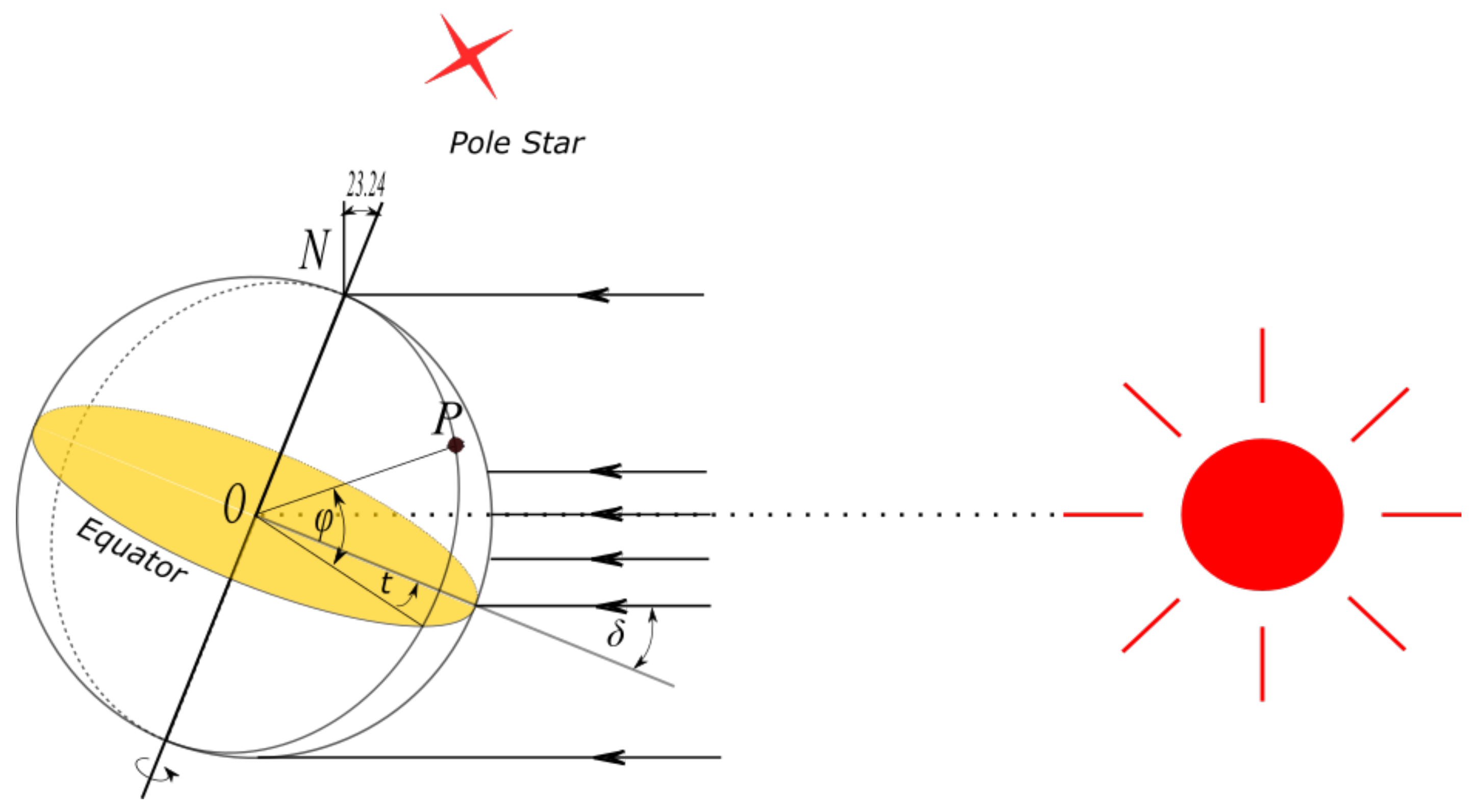
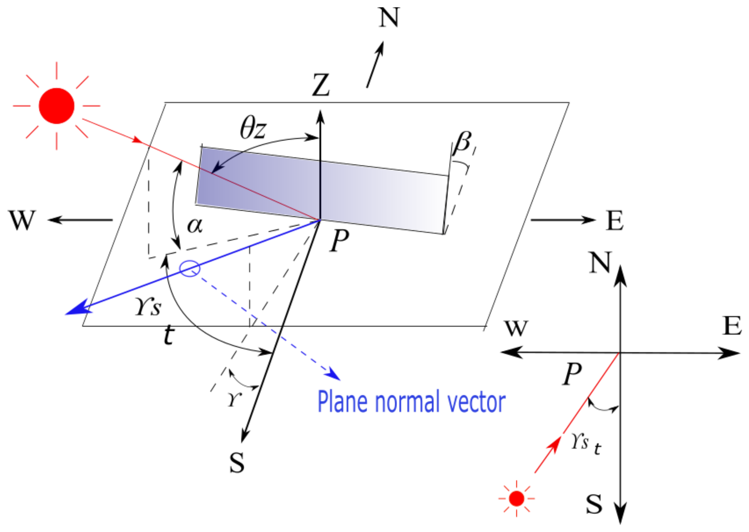
3. Inclined Surface Solar Radiation Calculation

With the proposal of the isotropic model by Liu and Jordan [21], there is an improvement of the Hay [17], Davis Keucher [18], and Reindl et al [26] models. In this paper, the isotropic model is used for simulation, and the accuracy of the model is also considered, the details of which are written below and illustrated using Figure 6 for easier understanding.

The total solar radiation ($T_s$) intercepted by a tilted plane is the sum of the direct radiation ($D_r$), the diffuse sky component ($D_f$), and the ground reflected radiation ($G_r$). They can be expressed as below:

$$T_s=D_r+D_f+G_r,$$

(4)

The direct radiation incident on an inclined surface is directly proportional to the direct radiation on the plane when the PV panel is horizontal, and it is given by:

$$D_r=H_d\frac{cos\theta }{cos{\theta }_z},$$

(5)

The sky diffuse radiation ($D_f$) and the ground reflected ($G_r$) components can be written as:

$$D_f=H_f\frac{1+cos\beta }{2},$$

(6)

and:

$$G_r=T_g\left(\frac{1-cos\beta }{2}\right)\rho .$$

(7)

where $H_d$ is the horizontal direct radiation, $H_f$ is the horizontal diffuse radiation, and $T_g$ is total ground horizontal radiation. The horizontal solar radiation data is given by NEDO [22]. $\rho$ is ground reflectivity.

$$\begin{array}{cc}\hfill cos\theta =& (sin\varphi cos\beta -cos\varphi sin\beta cos\gamma )sin\delta \hfill \\ \hfill +& (cos\varphi cos\beta +sin\varphi sin\beta cos\gamma )cos\delta cos\tau \hfill \\ \hfill +& cos\delta sin\beta sin\gamma sin\tau \hfill \end{array}$$

(8)

$$cos{\theta }_z=sin\varphi sin\delta +cos\varphi cos\delta cos\tau$$

(9)

4. PV Model

Singh et al. [27] and Jordehi et al. [28] wrote extensive review reports for solar PV, and the typical I–V characteristic of a PV array is given by the following equation:

$$I=N_p{I}_{ph}-N_p{I}_d[exp(\frac{qV}{kTA{N}_s}-1)]$$

(10)

$$I_{ph}=[I_{scr}+K_i(T-T_c)]\frac{T_s}{100}$$

(11)

$$I_d=I_c{\left(\frac{T}{T_c}\right)}^{3}exp\left[\left(\frac{q{E}_g}{KA}\right)(\frac{1}{T_c}-\frac{1}{T})\right]$$

(12)

$$I_c=\frac{I_{sc}}{exp(V_{oc}/AV)-1}$$

(13)

$$V=\frac{N_{s}KT}{q}$$

(14)

where:

• I—The PV output current;
• $I_{ph}$—The photo current;
• V—The PV output voltage;
• $N_s$—The number of cells connected in series;
• $N_p$—The number of modules connected in parallel;
• q—The charge of an electron;
• k—The boltzman’s constant;
• A—The pn junction ideality factor;
• $I_d$—The cell reverse saturation current;
• T—The cell temperature;
• $T_c$—The cell reference temperature;
• $I_c$—The reverse saturation current at $T_c$;
• $E_g$—The band gap energy of the semiconductor;
• $I_{scr}$—The cell short circuit current;
• $K_i$—The short circuit current temperature coefficient;
• $T_s$—The solar radiation in MWh/m²;

and the values of the parameter are shown in

Table 3. Rated power and constant values of PV.

P	250 W
$I_{sc}$	8.91 A
$I_{ph}$	8.214 A
$V_{oc}$	37.27 V
$K_i$	0.0032
$E_g$	1.12 eV
A	1.3
K	1.381 × 10${}^{-23}$ J/K
q	1.602 × 10${}^{-19}$ C

.

5. Effective Area

While calculating the area of the solar panels, the influence of the solar panel’s shadow should be considered, because the length of the shadow changes with the seasons and daily time. In order not to affect the amount of electricity generated, Naha City in Japan and Shenyang City in China were selected during winter solstice from 09:00 to 10:00. The shadow length corresponding to the 1-meter building is 1.811 m in Naha and 2.675 m in Shenyang and can be calculated via Equation (16).

The area parameters for both PV panel arrangements can be calculated using the following equations:

$$D_a=L_s\times (L_{a}sin\beta +h_g),$$

(15)

$$L_s=1/tan\left(\alpha \right),$$

(16)

$$L_a=l_p\times N_l,$$

(17)

$$W_a=w_p\times N_w,$$

(18)

According to the S-shape array shown in Figure 7, the area S is calculated as:

$$S=W_a\times (L_{a}cos\left({\beta }_s\right)+D_a).$$

(19)

From Figure 8, the area for the M-shape array $S_M$ is calculated as:

$$S_M=W_a\times L_{a}cos\left({\beta }_m\right).$$

(20)

Further, the solar elevation angles of Naha and Shenyang winter solstice are shown in

Table 4. The solar elevation angle ($\alpha$) in winter solstice (22 December) in Naha and Shenyang.

Time	9:00	9:15	9:30	9:45	10:00
Naha [${}^{\circ }$]	19.48	22.00	24.42	26.73	28.91
Shenyang [${}^{\circ }$]	14.59	16.26	17.81	19.23	20.50

[29]; and the parameters of the panel are defined in

Table 5. Constant values for footprint.

Height$h_g$	0.6 m
Angle of inclination${\theta }_a$	17${}^{\circ }$
Panel’s width$l_p$	1 m
Panel’s length$w_p$	1.65 m

.

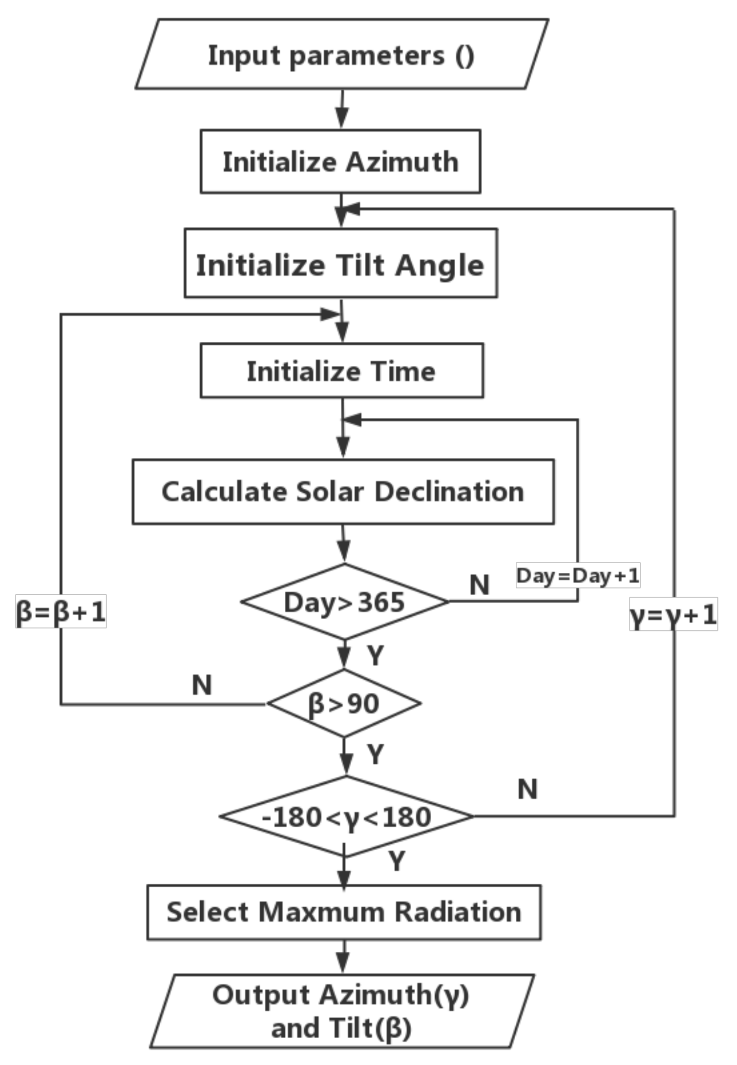
6. Simulation Condition and Steps

The following six different regions of Asia—Thailand (Bangkok), China (HongKong), Japan (Naha), Korea (Jeju), China (Shenyang), and Mongolia (Darkhan)—were selected for system simulation. The location details of each city are given in

Table 6. Location information for each simulation area.

Country	Region	North Latitude [${}^{\circ }$]	East Longitude [${}^{\circ }$]
Mongolian	Darkhan	49.46	105.97
China	Shenyang	41.798	123.43
Korea	Jeju	33.489	126.498
Japan	Naha	26.207	127.685
China	HongKong	22.25	114.25
Thailand	Bangkok	13.75	100.5

.

In the northern hemisphere, the range of latitude $\varphi$ is from 0 to 90${}^{\circ }$, the tilt angle $\beta$ of the PV array is between 0 and 180${}^{\circ }$, and the azimuth $\gamma$ varies between −180${}^{\circ }$ and 180${}^{\circ }$. In this paper, a multi-parameter optimization and a performance prediction program were developed. The traversal search method was used to start at a certain latitude angle $\varphi$. The tilt angle $\beta$ of the PV array is in the range of 0 to 90${}^{\circ }$, and the azimuth $\gamma$ is in the range of −180${}^{\circ }$ to 180${}^{\circ }$. The corresponding amount of irradiation under each tilt angle and the azimuth angle is calculated according to the method for calculating the amount of radiation on the inclined plane in Section 3, and the maximum amount of annual solar radiation was determined. The corresponding tilt angle and azimuth angle are the most preferred ones, and the above calculation process is represented in Figure 9.

The rated output of the power conditioner subsystem is set as 10 kW; the S-shape and M-shape panel arrangement is simulated in the six regions, and the overloaded rate is shown in

Table 7. Overloaded rate of panels.

Number of panels	40	50	60	70	80	90	100
Overloaded rate	100%	125%	150%	175%	200%	225%	250%

. The procedure can be represented by the following steps:

Step 1. According to the flow chart, calculate the amount of solar radiation that can be accepted in each direction of the S-shape and the M-shape. The optimum azimuth and the optimum tilt angle for the S-shape are obtained. Similarly, the optimum azimuth and tilt angle are also obtained for the M-shape. (The M-shape solar radiation calculation combines two 1 m² panels with tilt angles in opposite direction. Hence, the result will show the sum of the solar radiation collected in both directions. Position the back of the M-shape as azimuth angle from 90${}^{\circ }$ to −90${}^{\circ }$.)

Step 2. Simulate the amount of electricity generated in the six regions a year. Under the geographical conditions of Naha City, two PV types’ economic benefits and feasibility are to be calculated. It is assumed that the lifetime of a PV system is 20 years. The cost of the equipment and the unit price of electricity sold are set as parameters in the

Table 8. Reference price.

Electricity Price	21 [Yen/kWh]
Panel Price	70,000 [Yen/piece]
PCS	210,000 [Yen]
Land Price	5000 [Yen/m2]

.

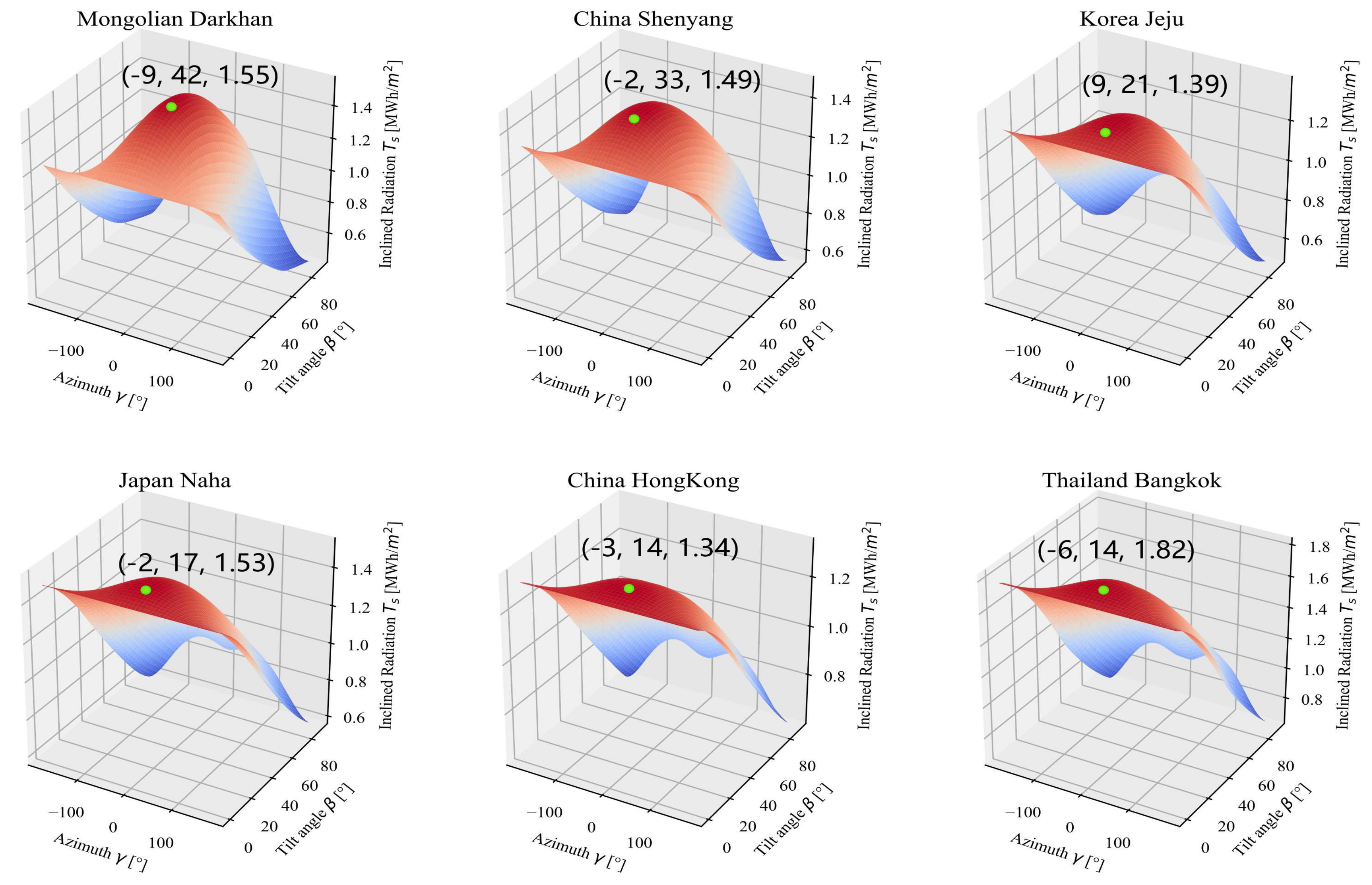
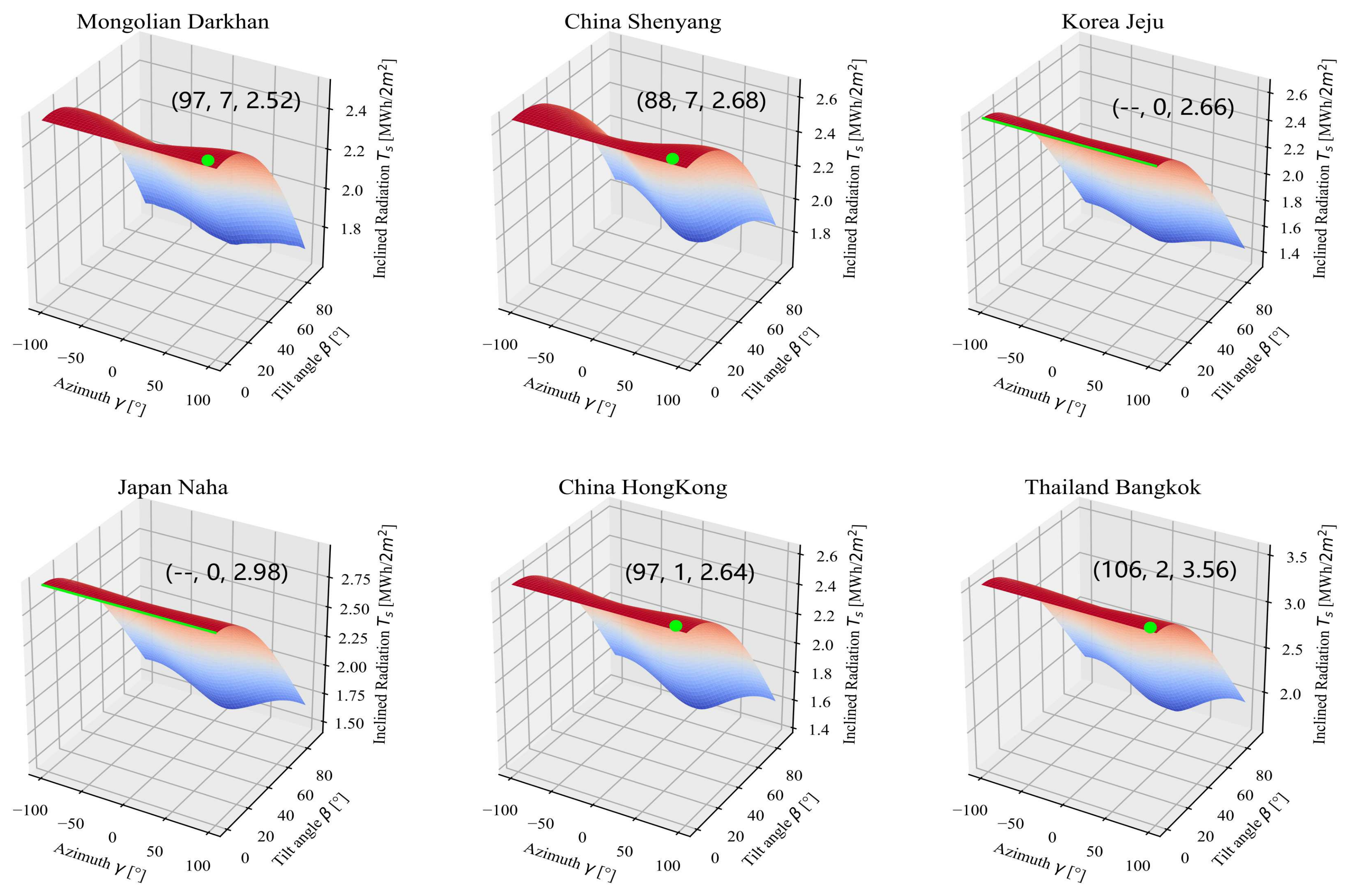
7. Results

Figure 10 and Figure 11 show the simulation results of the S-shape and M-shape panel setting, respectively. The optimal tilt and azimuth angle for each region was obtained. The azimuth angle should be 0, but the actual data are affected by weather and geographical location, which also affects the simulation results. It can be observed from Figure 10 that the amount of solar radiation received on both sides of the east and the west is symmetrical about the azimuth 0 direction. To show the result accurately,

Table 9. Comparison results of optimal angles for the PV panel with the Industrial Technology Development Organization (NEDO).

City Name	NEDO Results [${}^{\circ }$]	Simulation Results [${}^{\circ }$]
Naha	Tilt 17.6${}^{\circ }$	Tilt 17${}^{\circ }$, Azimuth $-2^{\circ }$
Akita	Tilt 26.2${}^{\circ }$	Tilt 27${}^{\circ }$, Azimuth $-2^{\circ }$
Fukuoka	Tilt 26.1${}^{\circ }$	Tilt 26${}^{\circ }$, Azimuth 10${}^{\circ }$
Kagoshima	Tilt 27.7${}^{\circ }$	Tilt 22${}^{\circ }$, Azimuth 0

has shown the result of NEDO [22] and this paper’s simulation result based on the optimal tilt angle in several areas provided by NEDO.

Table 10. The S-shape’s optimal azimuth, tilt angle, and maximum of solar radiation for each simulation area.

Region	Azimuth [${}^{\circ }$]	Tilt [${}^{\circ }$]	Radiation [MWh/m2]
Darkhan	−9	42	1.55
Shenyang	−2	33	1.49
Jeju	9	21	1.39
Naha	−2	17	1.53
HongKong	−3	14	1.34
Bangkok	−6	14	1.82

and

Table 11. The M-shape’s optimal azimuth, tilt angle, and maximum of solar radiation for each simulation area.

Region	Azimuth [${}^{\circ }$]	Tilt [${}^{\circ }$]	Radiation [MWh/2m2]
Darkhan	97	7	2.52
Shenyang	88	7	2.68
Jeju	–	0	2.66
Naha	–	0	2.98
HongKong	97	1	2.64
Bangkok	106	2	3.56

display the optimal tilt azimuth angle of two types of PV array, respectively. The results of the M-shape show that the optimal tilt angle is close to 0. This means that when we make two pieces of PV panels as a group, the optimal tilt angle will let the PV array almost be at surface level. It is easy for the PV array to accumulate dust rain and snow in an actual situation, and it can also be easily destroyed in harsh environments.

Based on different optimal tilt angles and calculation methods, there are variations in results, especially in the case of Kagoshima. However, NEDO’s calculation approach considered a large area, and the optimal tilt angle is based on approximation; hence, the results obtained in this study are reliable. Hong Kong’s optimal tilt angle was determined to be the same as that of Bangkok. This is because they are both closer to the equator, and hence, the optimal tilt angle will be close to the local latitude.

Table 12. Simulation result of the M-shape array in six areas.

City		Direction	(0,180${}^{\circ }$)	(45${}^{\circ }$, −135${}^{\circ }$)	(135${}^{\circ }$, −45${}^{\circ }$)	(90${}^{\circ }$, −90${}^{\circ }$)
	Pieces
Darkhan	80		21.19 MWh	21.31 MWh	21.31 MWh	21.48 MWh
	100		24.33 MWh	24.48 MWh	24.48 MWh	24.69 MWh
Shenyang	80		23.43 MWh	23.87 MWh	23.85 MWh	24.22 MWh
	100		26.97 MWh	27.51 MWh	27.48 MWh	27.94 MWh
Jeju	80		21.61 MWh	21.71 MWh	21.69 MWh	21.76 MWh
	100		24.10 MWh	24.22 MWh	24.20 MWh	24.28 MWh
Naha	80		24.13 MWh	24.22 MWh	24.22 MWh	24.30 MWh
	100		26.79 MWh	26.90 MWh	26.91 MWh	27.00 MWh
Hongkong	80		23.25 MWh	23.25 MWh	23.36 MWh	23.43 MWh
	100		26.44 MWh	26.90 MWh	26.91 MWh	27.00 MWh
Bankok	80		27.89 MWh	27.93 MWh	27.95 MWh	27.99 MWh
	100		30.22 MWh	30.27 MWh	30.29 MWh	30.34 MWh

shows the four directions of the M-shape, which are north–south (0,180${}^{\circ }$), northeast– southwest (45${}^{\circ }$,−135${}^{\circ }$), southeast–northwest (135${}^{\circ }$,−45${}^{\circ }$) and east–west (90${}^{\circ }$,−90${}^{\circ }$) respectively. The overload rate is set at 200% and 250%. Additionally, the optimal azimuth angle of each direction is also calculated in this step. The tilt angle of Darkhan and Shenyang is 25${}^{\circ }$, Jeju and Naha is 20${}^{\circ }$, Hongkong and Bankok is 15${}^{\circ }$. The results for west–east and optimal–azimuth are almost the same when compared.

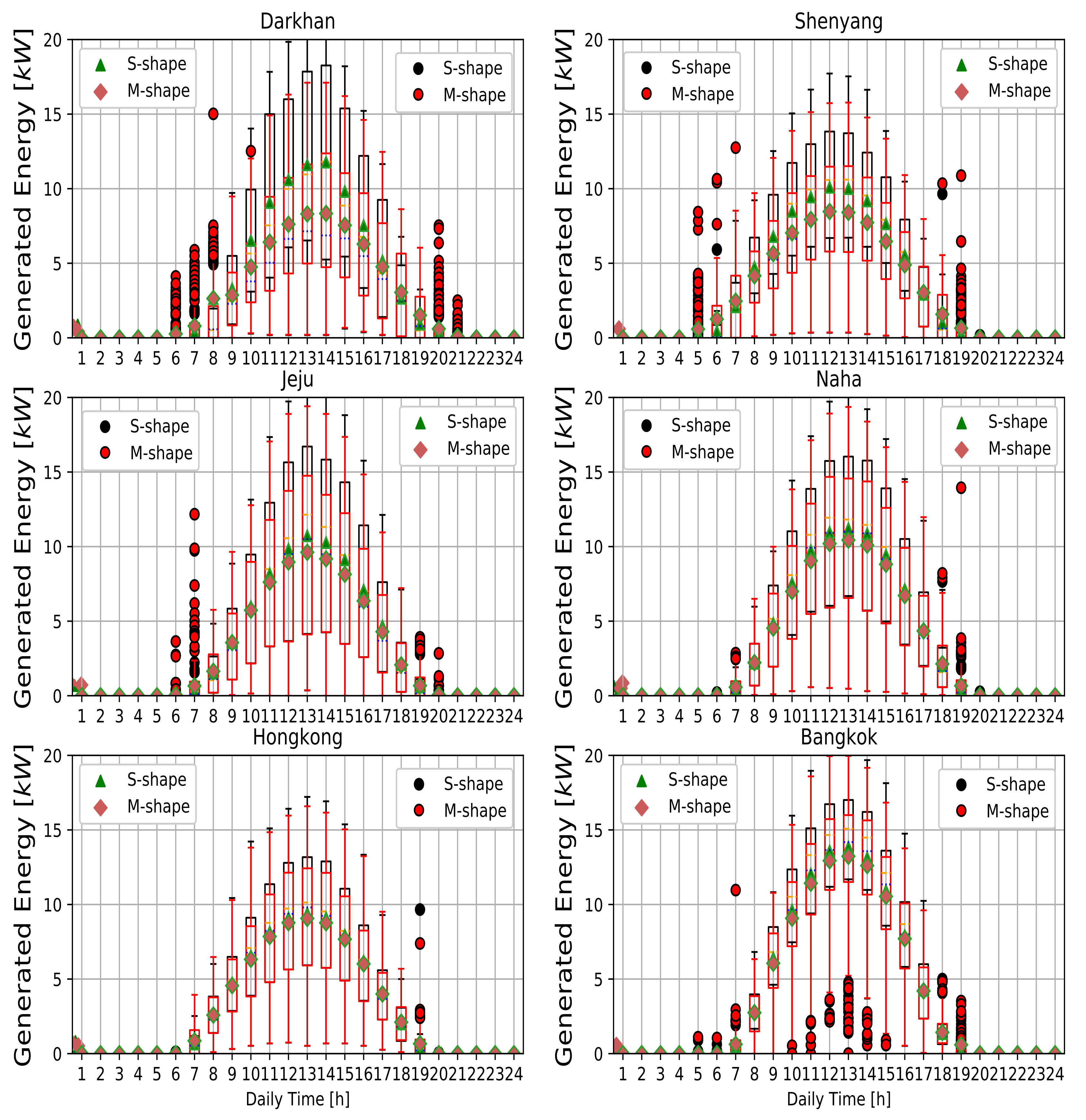
Figure 12 shows the two types of daily power generation characteristics throughout one year, which are under the number of the same panels (80) and in siz different latitude regions. It can be seen that at mid-latitudes (Darkhan, Shenyang, Jeju), the overall graphic shape is similar to the situation described in Figure 1. It is well explained here that the M-shape can effectively reduce the overload rate when the solar radiation is strong at solar noon and increases power generation in the morning and at nightfall. This indicates that the M-shape can increase the amount of power generation while controlling the overload rate. At lower latitudes (Naha, Hongkong, Bangkok), the graphic features of the M-shape and S-shape will be closer. It can be seen that the M-shape does not have an impact on the traditionally designed power generation but shows a good advantage in terms of area savings.

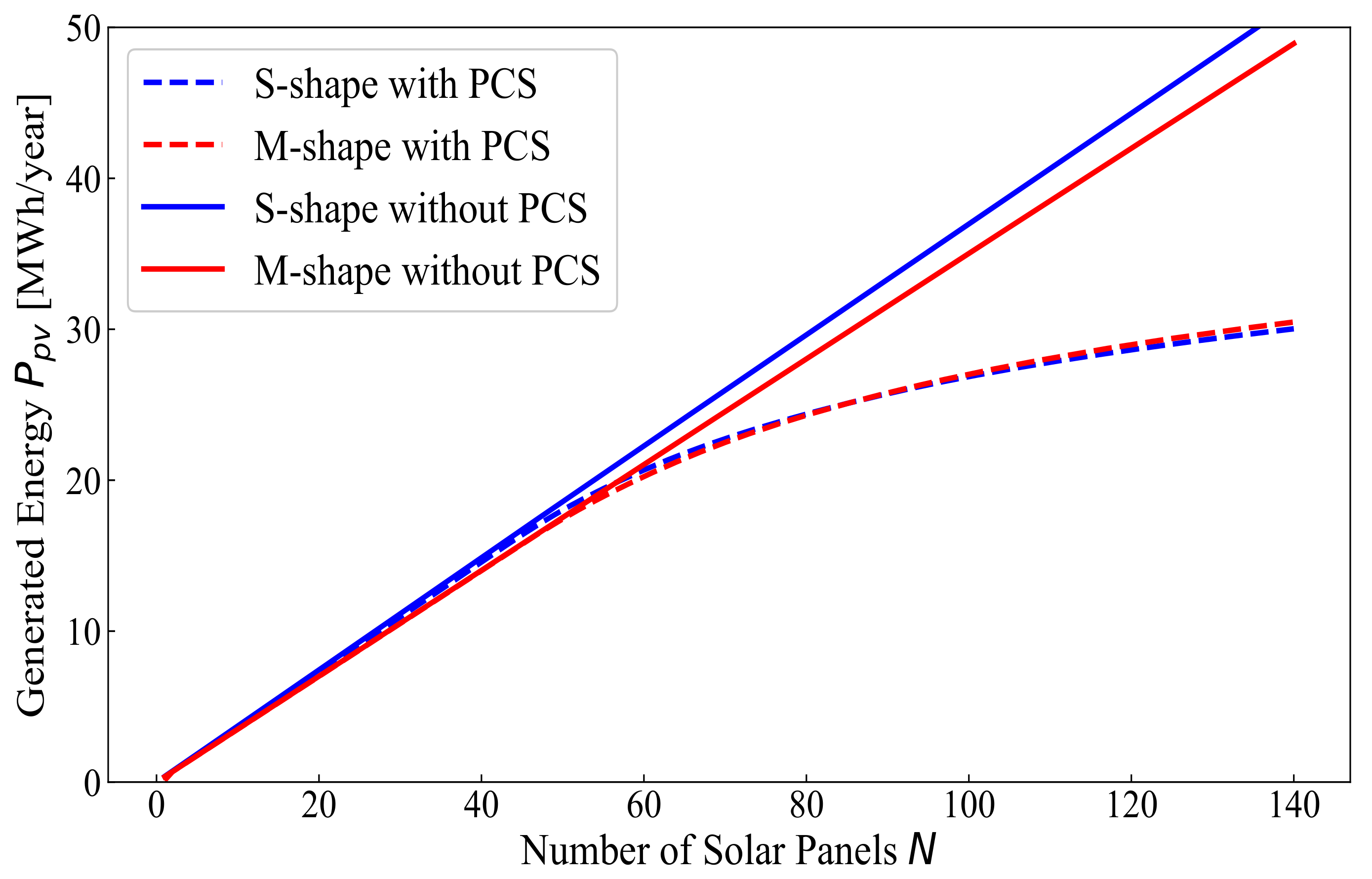
Figure 13 shows the generated power of the S-shape, M-shape, and two types’ maximum output without PCS. The blue and red lines show the S-shape and M-shape power generation characteristics, respectively. On the one hand, they show that without PCS, the S-shape output power is growing faster. When the number of panels is over 40 (overload rate 100%), the gap between without PCS generation and actual power generation is growing. They also show that before around 90 (overload rate 225%) solar panels, the S-shape power generation is more than that of the M-shape. This is for the same pieces of PV panels; S-shapes are set at an optimal tilt angle, while M-shapes are set as a group of solar panels. However, after overloading beyond 225%, the M-shape becomes better than the S-shape. Since both the M-shape and S-shape will exceed the rating of PCS when the sun is strong at solar noon, power generation in this part is the same. M-shapes, however, collect energy better in the morning and afternoon. The power generation efficiency of the S-shape will show better benefits. Another important factor is the geographic location. The figure shows the amount of power generated by Naha. From Figure 12, it can be concluded that with increasing latitude, the M-shape will have a better power generation effect than this result.

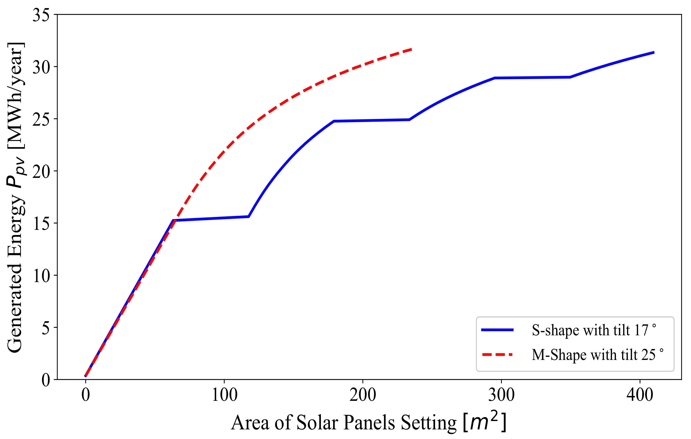
Figure 14 shows the area usage of two types of PV panels. The M-shape PV design uses less area space compared to the S-shape design. This is due to the concept that M-shapes are continuous, while S-shape uses intervals. The horizontal line in Figure 14 indicates the increase of area without power generation. This will lead to increased costs with less revenue. As the number of solar panels increases, the efficiency of the M-shape becomes larger.

Table 13. Area comparison of the M-shape and S-shape in Shenyang and Naha.

Type	Shenyang				Naha
	40	80	120	160	40	80	120	160
M-shape	59.8 m2	119.6 m2	179.4 m2	239.3 m2	62.0 m2	124.0 m2	186.1 m2	248.1 m2
S-shape	55.4 m2	233.3 m2	411.3 m2	589.3 m2	63.1 m2	179.1 m2	295.2 m2	411.2 m2

shows the detailed area usage for the two PV arrangements for Naha and Shenyang. Another point is that as latitude increases, the sun’s elevation angle becomes smaller. This makes the shadow length larger and verifies that the M-shape will greatly reduce the area in mid-latitude.

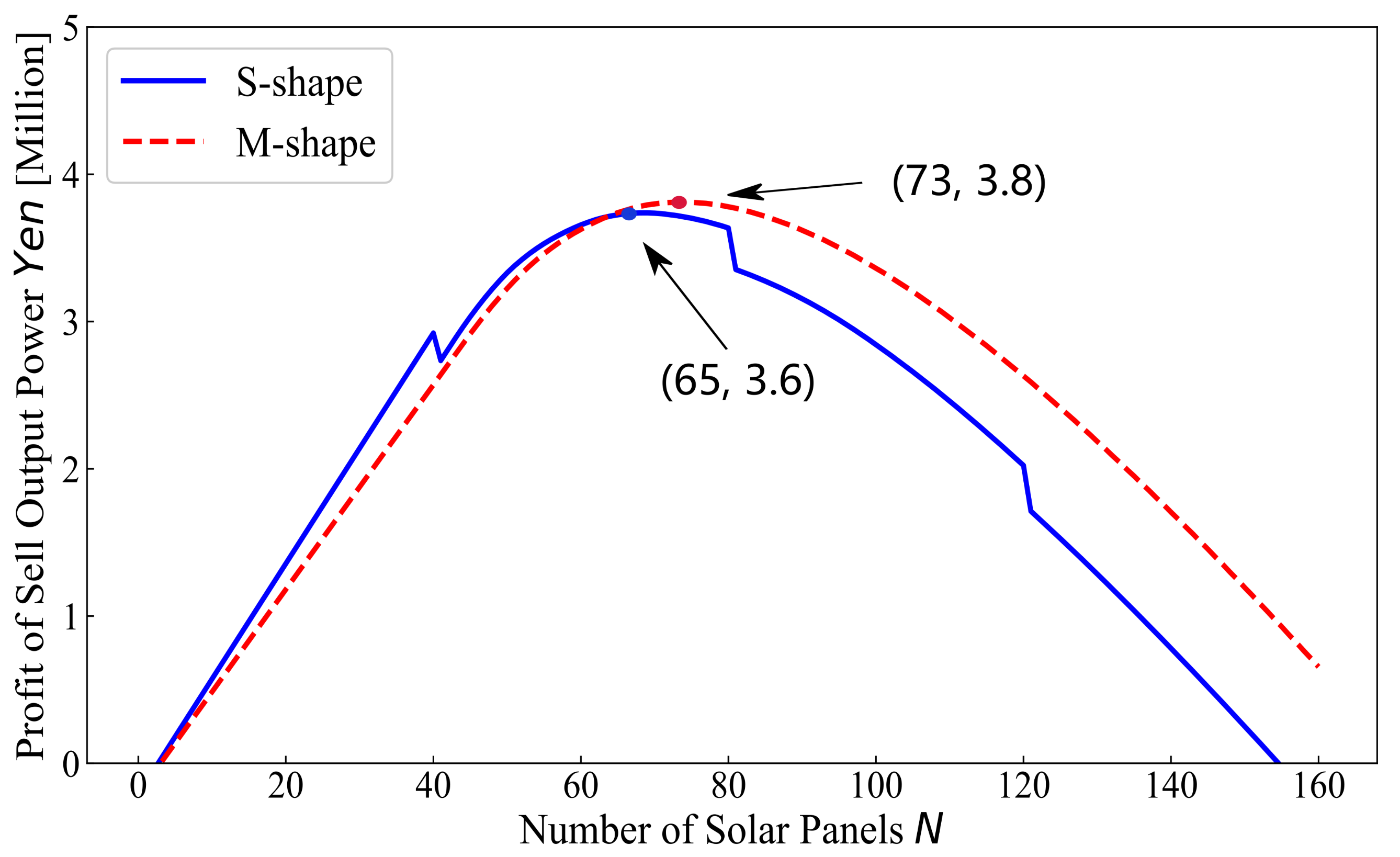
Figure 15 clearly shows the the M-shape and S-shape that are considered as the best economical solutions. As the number of panels increases, the power generation increases due to an overload of around 200% leading to a profit. If the overload exceeds 200%, it could lead to a downward trend affecting cost. The descending line represents the cost of land. According to the simulation result, 73 pieces of solar panels used in the M-shape design are optimal. The power generation is 23 MWh, the profit is 3.8 million yen, and the floor area is 114 m². The overload rate is 182.5%. Similarly for the S-shape, 65 solar panels are an optimal choice. The power generation is 22 MWh, the profit is 3.6 million yen, and the floor area is 162 m². The overload rate was 172.5%. It can be confirmed that the installation of the west–east setting can save space and be profitable.

8. Conclusions

This paper showed a modern design approach for improving PV system power generation efficiency by changing the traditional design of PV arrangement. The proposed scheme was applied to six Asian cities to confirm its robustness and effectiveness. The optimal tilt angles of the S-shape in the six regions are Bangkok (14${}^{\circ }$), Hong Kong (14${}^{\circ }$), Naha (17${}^{\circ }$), Jeju (21${}^{\circ }$), Shenyang (23${}^{\circ }$), and Darkhan (42${}^{\circ }$). The optimal tilt angle of M-shape tends to zero. However, considering the environmental factors, the angle degree of M-shape was given 15${}^{\circ }$ to 25${}^{\circ }$ during the simulation. Moreover, detailed analysis for all case studies was presented with applying different overload rates to ensure the capability of the proposed in different operating conditions even severe ones. This paper’s simulation results proved that the east–west direction is the best for M-shape and indicated that the M-shape can save more than half the area of the traditional S-shape. As the latitude increases, the shadow length increases, and the M-shape can make better use of this advantage. When the rated power of the PCS is 10kW and the overload rate reaches 225%, the power generation efficiency of the M-shape exceeds the conventional S-shape. Analysis of the profit situation over 20 years in Naha shows that the M-shape will be higher than the S-shape. Although this result is small (increase of 0.2 million yen), it is undeniable that the M-shape will improve economic efficiency. Here, that distributed generation accounts for a large proportion, and most of them are based on home roofs and small yards. The area is difficult to change here, so adding solar panels to increase output power is important, and the M-shape is prepared for this. This article analyzed the M-shape regarding its geographical location, floor area, power generation efficiency, and economic benefits. We can confidently point out that the PV array will enter the beginning of the M-shape era, and there will be many problems waiting to be solved.