Article

AISAC: An Artificial Immune System for Associative Classification Applied to Breast Cancer Detection

by
David González-Patiño
1,
Yenny Villuendas-Rey
2,*,
Amadeo José Argüelles-Cruz
1,*,
Oscar Camacho-Nieto
2,* and
Cornelio Yáñez-Márquez
1,*
1
Centro de Investigación en Computación, Instituto Politécnico Nacional, CDMX 07738, Mexico
2
Centro de Innovación y Desarrollo Tecnológico en Cómputo, Instituto Politécnico Nacional, CDMX 07700, Mexico
*
Authors to whom correspondence should be addressed.
Appl. Sci. 2020, 10(2), 515; https://doi.org/10.3390/app10020515
Submission received: 17 November 2019 / Revised: 22 December 2019 / Accepted: 6 January 2020 / Published: 10 January 2020
(This article belongs to the Special Issue Signal Processing and Machine Learning for Biomedical Data)

Abstract

:
Early breast cancer diagnosis is crucial, as it can prevent further complications and save the life of the patient by treating the disease at its most curable stage. In this paper, we propose a new artificial immune system model for associative classification with competitive performance for breast cancer detection. The proposed model has its foundations in the biological immune system; it mimics the detection skills of the immune system to provide correct identification of antigens. The Wilcoxon test was used to identify the statistically significant differences between our proposal and other classification algorithms based on the same bio-inspired model. These statistical tests evidenced the enhanced performance shown by the proposed model by outperforming other immune-based algorithms. The proposed model proved to be competitive with respect to other well-known classification models. In addition, the model benefits from a low computational cost. The success of this model for classification tasks shows that swarm intelligence is useful for this kind of problem, and that it is not limited to optimization tasks.

1. Introduction

Evolutionary computation (EC) is an active research area with several successful applications in a variety of domains [1,2,3]. Evolutionary methods have exhibited impressive performances when compared to other approaches.
One branch of evolutionary methods, known as swarm intelligence (SI), has shown the ability to find accurate solutions to numerous problems, such as computer vision [4], feature selection [5], clustering [6], network routing [7], and resource planning [8], among others.
However, regarding supervised classification, SI has been applied mainly for parameter optimization of classifiers (Support Vector Machines [9], Gamma [10], fuzzy rule-based classifiers [11]), for training set instance selection (for neural networks [12], k-nearest neighbors [13], and Support Vector Machines [14]), and in other optimization problems: attribute and instance selection [15,16], and the selection of optimal parameter values [17]. Despite the rich application of SI in the field, there is currently no algorithm based on SI that correctly classifies any presented dataset, as a consequence of the no free lunch theorem [18].
Although some works have been developed in this area, such as immune system models [19], immune networks [20], and, more recently, endocrine systems [21], this is an under-researched area.
For this reason, we propose a new model based on the biological immune system designed explicitly for classification. The aim of this system is to overcome the limitations of previous models and be competitive with well-known classification models. Our model constitutes a contribution to the state of the art on novel pattern classifiers, and tackles some challenges in the field of evolutionary pattern recognition and related applications.
The main contribution of this research is a model of immune system classification which is statistically significantly better than other immune-based classifiers. The proposed model is also competitive with respect to classifiers such as multilayer perceptron [22], Support Vector Machines [23], C4.5 [24], and random forest [25]. In addition, it has a low computational cost, is highly configurable, and performs well for an impactful application area: the early detection of breast cancer.
The rest of the paper is structured as follows. In Section 2, a review of the related works is presented. General elements of the human immune system are detailed in Section 3, as well as the new Artificial Immune System for Associative Classification (AISAC). Then, Section 4 details the experiments where the proposed model is applied to medical data analysis, in particular to the detection of breast cancer, as well as other types of cancer. The results obtained are compared to other classification models based on immune systems, in addition to other well-known classification systems. Furthermore, empirical studies are performed in order to determine the adequate parameter values for the proposed AISAC, which are detailed in Section 4.2. In Section 5, a discussion of the results is presented. The paper finishes by offering conclusions and future lines of work in the Conclusions section.

2. Related Works

We compared ten learning classification systems to our AISAC model. We selected three immune-based classification algorithms (AIRS1 [26], Immunos1 [27], and CLONALG [28]), as well as six well-known algorithms, considered among the best general-purpose classifiers (Support Vector Machines [23], multilayer perceptron [22], nearest neighbor [29], RIPPER [30], C4.5 [24], naïve Bayes [31], and random forest [25]).
All the algorithms were available in Weka [32], including the immune-based algorithms, which were released by Jason Brownlee in 2011, with a recent update in 2013 [27]. We manually explored the best parameter configuration for each algorithm. In the following paragraphs we offer a brief description of the learning algorithms.

2.1. Supervised Classifier

In the literature there are several classification algorithms, belonging to different approaches. In this section we will address seven of them; these algorithms represent vector support machines, neural networks, distance-based classifiers, decision trees, probabilistic classifiers, rule-based classifiers, and classifier committees.
Support Vector Machines (SVM) [23] are algorithms which construct a model that linearly separates classes using a hyperplane. The classification performance depends on the separation done by the hyperplane. This algorithm is designed to work with two classes, so in order to use a multiclass dataset, other strategies have been used, such as multi-splitting the classes or constructing more than one model to cover all the classes. Finding the right kernel is not easy, so the results may vary. SVM models suffer from a lack of interpretability. We used the Weka implementation of IMO due to its low computational cost.
Multilayer perceptron (MLP) [22] is an artificial neural network model which maps a set of inputs to get a defined set of outputs. This model has multiple layers and nodes representing neurons that are connected in each layer. Back propagation is an algorithm used to train multilayer neural networks by changing the weights in each connection using the error of the outputs, which is propagated to each previous layer. Training can become a very expensive process, since it requires a long time and a large amount of data to be trained; in addition, the generated model is not very interpretable.
The nearest neighbor (NN) [29] algorithm computes the distances between the test pattern and all the training patterns, and chooses the dominant class among the k-nearest patterns. This algorithm is one of the simplest machine learning algorithms; despite this fact, the performance of this algorithm is one of the highest for some datasets. This algorithm suffers from high memory consumption, since the training set is kept in memory at all times.
Repeated Incremental Pruning to Produce Error Reduction (RIPPER) [30] is an algorithm based on generating association rules for reducing the error when pruning. The generation of rules is made by applying a pruning operator to delete conditions or rules in order to obtain the greatest reduction of error. The output model is easy to understand.
C4.5 [24] is a decision tree for pattern classification. The information entropy is used to choose the node splits to generate the tree, where each node represents an attribute of the data. This algorithm may become stuck at a local minimum and would need additional processes to avoid this. The output model is easy to understand.
Naïve Bayes [31] is a classifier based on the Bayes theorem and assumes the independency of each attribute. This algorithm requires a small quantity of training data to generate the model used for classification.
Random forest [25] is a classifier ensemble based on a random combination of tree classifiers, such that each tree depends on the values of an independently tested random classification tree. It is a small modification of bagging that builds a long collection of uncorrelated trees and then averages the results.

2.2. Classification Systems Based on Immune Systems

The Artificial Immune Recognition System (AIRS) [26] is inspired by the immune system and uses memory cells, resource competition, affinity maturation, and clonal selection, based on the functioning of the biological immune system. This algorithm has four stages, which are data normalization and initialization, memory cell identification and artificial recognition balls generation, competition for resources, and conversion of candidate memory cells into memory cells.
Immunos1 [27] is a model based on the immune system that exhibits dynamic learning and assumes no data reduction. The training population is partitioned and allows independent and parallel management in the classifier. The cells compete by calculating the affinity using Euclidean distance and calculating the avidity.
CLONALG [28] is based on the clonal selection principle, which allows the cells that correctly recognize the antigens to proliferate. It has the ability to perform parallel search and is used for pattern recognition and optimization problems using each antibody as a candidate for the optimal solution.
Our proposal differs from other classification algorithms due to the use of stochastic methodologies, which make it possible to find solutions to non-polynomial problems. Likewise, this behavior allows the algorithm to explore and find optimal solutions to perform the corresponding classification.

3. Our Proposal: An Artificial Immune System for Associative Classification

3.1. The Human Immune System

The immune system is a biological system that protects an organism against pathogens, such as biological, chemical, or intern hazards [33]. The immune system has two main functions: to recognize substances foreign to the body (also called antigens), and to react against them. These substances may be microorganisms that cause infectious diseases, transplanted organs or tissues of another individual, or tumors. The proper functioning of the immune system provides protection against infectious diseases and can protect a person from cancer.
An antigen is any substance that causes the body to create antibodies. It is a substance capable of inducing an immune response. Among the properties of antigens, the following can be highlighted [34]:
  • They have to possess the quality of strangers to the human body. That is, the antigens may come from outside (exogenous) or they may be generated in our body (endogenous);
  • Not all trigger an immune response, because of the amount of inoculum that is introduced. A considerable proportion is needed to trigger a response;
  • The immune response is under genetic control. Because of this, the immune system decides whether to respond or not, and against whom it will respond and against whom it will not;
  • The basic structure has an important relevance. This is because T and B lymphocytes are involved in cell-mediated immunity: T lymphocytes regulate the entire immune response, and B lymphocytes are secondary;
  • Some antigens must be recognized by the T lymphocytes to give a response, which are called antigens of thymus-dependent type; there are others that do not—it is enough for them to reach the B lymphocyte to be recognized as such. These are called thymus-independent antigens.
Antigenic macromolecules have two fundamental elements: the antigenic carrier, which is a macroprotein, and the antigenic determinants (epitopes), which are small molecules attached to them with a particular spatial configuration that can be identified by an antibody; therefore, the epitopes are responsible for the specificity of the antigen for the antibody.
Thus, the same antigenic molecule can induce the production of as many different antibody molecules as different antigenic determinants it possesses. For this reason, antigens are said to be polyvalent. Generally, an antigen has between five and ten antigenic determinants on its surface (although some have 200 or more), which may be different from each other so that they may react with different types of antibodies.
The immune system is divided into two subsystems: the innate immune system and the adaptive immune system. The innate immune system can detect antigens inside the system, while the adaptive immune system is more complex, since it exhibits a response which can be modified to answer back to specific antigens. This response is improved by the repeated presence of the same antigen.
The innate immune system has an immediate response, but this is not specific and there are no memory cells involved. In contrast, the adaptive immune system response takes more time to be activated but is specific to the antigen because memory cells are involved.
Adaptive immunity or acquired immunity is the ability of the immune system to adapt, over time, to the recognition of specific pathogens with greater efficiency [35]. Immunological memory is created from the primary response to a specific pathogen and allows the system to develop a better response to eventual future encounters.
Antibodies are chemicals that help destroy pathogens and neutralize their toxins. An antibody is a protein produced by the body in response to the presence of an antigen, and it is able to combine effectively with it. An antibody is essentially the complement of an antigen.
The specific adjustment of the antibody to the antigen depends not only on the size and shape of the antigenic determinant site, but also on the site corresponding to the antibody, more similar to the analogy of a lock and key. An antibody, as well as an antigen, also has a valence. While most of the antigens are polyvalent, the antibodies are bivalent or polyvalent. Most human antibodies are bivalent.
Various cell types carry out immune responses by way of the soluble molecules they secrete. Although lymphocytes are essential in all immune responses, other cell types also play a role [35]. Lymphocytes are a special group of white blood cells: they are the cells that intervene in the defense mechanisms and in the immune reactions of the organism.
There are two main categories of lymphocytes: B and T [35].
B lymphocytes, which represent between 10% and 20% of the total population, circulate in the blood and are transformed into antibody-producing plasma cells in the event of infection. They are responsible for humoral immunity. T lymphocytes are divided into two groups that perform different functions:
  • T lymphocyte killers (killer cells or suppressor cells) are activated by abnormal cells (tumor or virus-infected); they attach to these cells and release toxic substances called lymphokines to destroy them;
  • T helper cells (collaborators) stimulate the activity of T-killer cells and intervene in other varied aspects of the immune reaction.
Macrophages (from Greek “big eaters”) are cells of the immune system that are located within tissues. These phagocytic cells process and present the antigens to the immune system. They come from precursors of bone marrow that pass into the blood (monocytes) and migrate to sites of inflammation or immune reactions. They differ greatly in size and shape depending on their location. They are mobile, adhere to surfaces, emit pseudopodia, and are capable of phagocytosis-pinocytosis or have the capacity to store foreign bodies.
When macrophages phagocyte a microbe, they process and secrete the antigens on their surface, which are recognized by helper T lymphocytes, which produce lymphokines that activate B lymphocytes. This is why macrophages are part of the antigen-presenting cells. Activated B lymphocytes produce and release antibodies specific for the antigens presented by the macrophage. These antibodies adhere to the antigens of the microbes or cells invaded by viruses, and thus attract with greater avidity the macrophages to phagocyte them [34].
Subsequently, the regulation phase controls the cells generated in the immune response in order to avoid damaging the system itself and preventing autoimmune responses. Finally, in the resolution phase, the harmful agent is removed and the cells generated to destroy the antigen die, only storing the memory cells.
The immune system has been the inspiration for numerous researchers in order to develop learning classifier systems [36,37,38,39]. Similarly, the immune system inspired the model proposed in this paper, the Artificial Immune System for Associative Classification, which is described in the next section.

3.2. AISAC: Artificial Immune System for Associative Classification

The main goal of classifier systems is to assign or predict a class label for an unseen pattern according to its attributes after training it with similar patterns [40].
Many classifier systems are based on two steps: model construction and model operation [41]. Model construction is a representation of the training set, which is used to generate a structure to classify the patterns presented. Model operation classifies data whose class labels are not known using the previously constructed model. In this paper, the classification problem is addressed by proposing a new model based on the immune system. Although numerous computational models have been developed based on the human immune system [42], this research presents a new model that incorporates additional elements of the immune response. The model is called Artificial Immune System for Associative Classification (AISAC). This model is proposed within the supervised classification paradigm, and therefore constitutes a new supervised classifier.
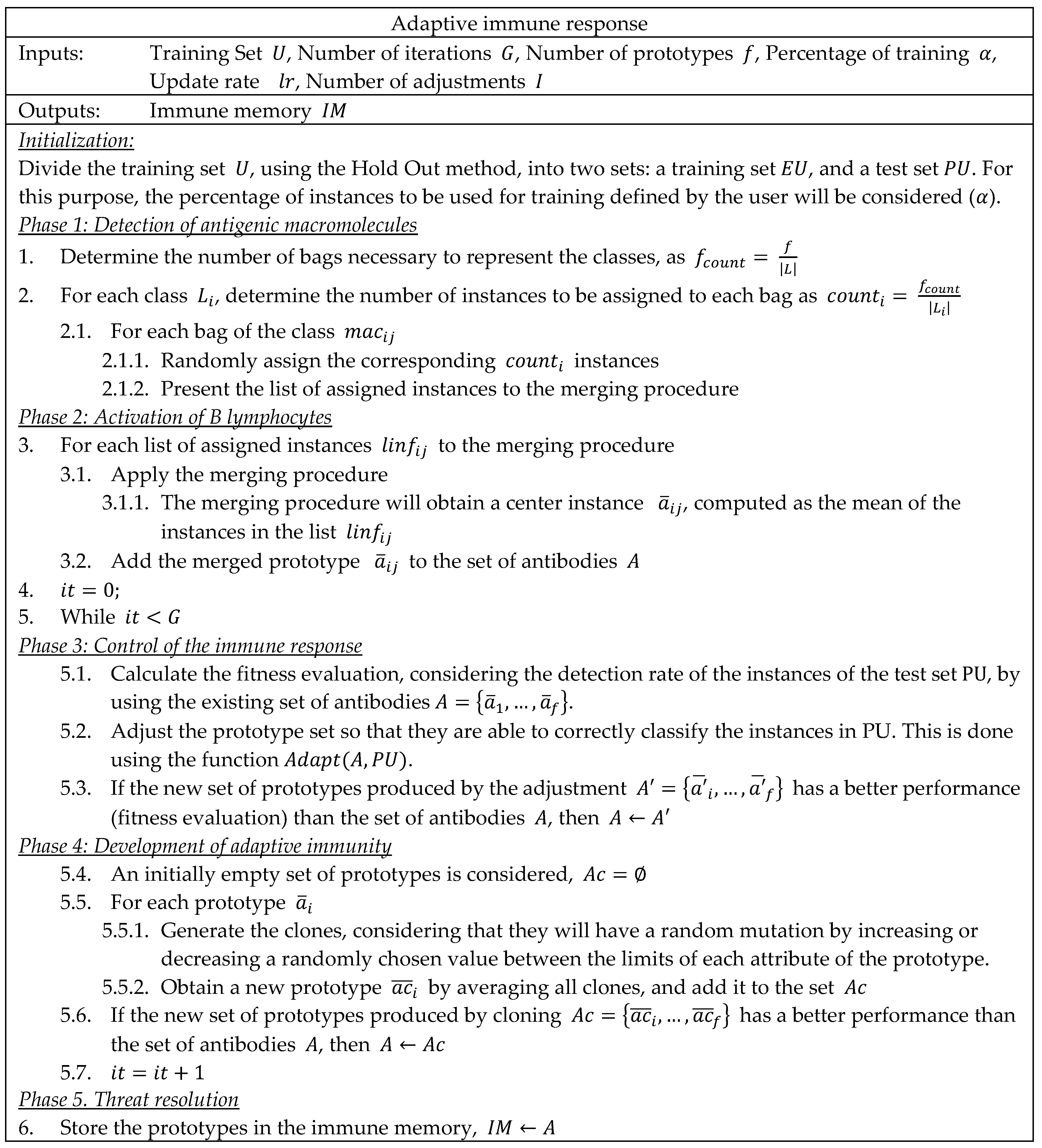
Among the characteristics of the proposed model, it can be highlighted that it is an eager classifier, since it generates internal data structures to classify the new instances. Thus, the training set is replaced by other structures. The proposed artificial immune system model includes two types of functions: the acquired (adaptive) immune response, and the innate immune response. The acquired immune response consists of five phases:
  • Detection of antigenic macromolecules;
  • Activation of B lymphocytes;
  • Immune response regulation;
  • Development of adaptive immunity;
  • Resolution of the threat.
The innate immune response has only one phase:
  • Resolution of the threat.
In general, the acquired immunological response begins with the detection of antigenic macromolecules by macrophages. Each macrophage will phagocytose a number of antigenic determinants of the antigenic molecule in which it specializes. Subsequently, each macrophage will present the antigenic determinants that it phagocytosed to the T lymphocyte helpers.
In Phase 2, these lymphocytes will generate an immune response, activating a certain number of B lymphocytes. Activated B lymphocytes will produce and release specific antibodies to the antigens presented by the macrophage. Then, the immune response will be monitored (Phase 3). If the immune response is satisfactory, the generated antibodies are conserved. Otherwise, a readjustment of the generated antibodies is performed so that they are able to combine with the antigenic determinants presented.
To guarantee the development of adaptive or acquired immunity (Phase 4), each of the antibodies will undergo a reconstitution phase so that it is capable of improving its immune response. Finally, in Phase 5, the antigenic macromolecules are completely removed and the antigens are stored in the immune memory.
In the case of the innate immune response a set of antibodies is already in memory; when an antigen is present, it is automatically detected and eliminated.

Metaphor-Free AISAC

The proposed artificial immune system-based model is indeed a classification algorithm. The acquired immune response corresponds to the model construction phase of the classifier, and the innate immune response corresponds to the model operation phase of the algorithm.
Thus, the training phase consists of five steps:
  • Detection of antigenic macromolecules. For each class (antigenic macromolecule), a selected number of instance bags (macrophages) will be computed. Then, the instances of the class will be randomly assigned to the bags;
  • Activation of B lymphocytes. For each bag of each class, a prototype (B lymphocyte) will be computed, considering the mean of the instances in the corresponding bag;
  • Immune response regulation. The prototypes computed in phase 2 are moved in the space by using the training set classification performance as an adaptability function;
  • Development of adaptive immunity. The prototypes are cloned, to obtain the desired number of candidate closed prototypes. Then, the best performed clone is kept;
  • Resolution of the threat. The final prototypes are stored as training data, and the original training set is deleted.
The innate immune response has only one phase:
  • Resolution of the threat. In here, the instance to classify is assigned to the class of its closets prototype.
The complete pseudocode of the model construction (adaptive immune response) in the proposed AISAC model is shown below in Figure 1. In this model, the following assumptions are made. First, we have a set of labeled training data   U = { u 1 , ,   u n } , where each instance is represented by a vector of attributes, features, or characteristics, u i = [ u i 1 , , u i m ] R m . This data set constitutes the antigenic determinants (instances), of the antigens to be detected. Each instance is associated with a single class to which it belongs, which is denoted as l ( u i ) .
The set of all classes within U is denoted as   L = { l 1 , ,   l k } . Each of these classes is considered a microprotein-carrying antigenity. The data of the test set P = { p 1 , ,   p t } is described by the same attributes or characteristics as the training data; thus, a test object is denoted by p i = [ p i 1 , , p i m ] R m .
The pseudocode of the adjustment in the adaptive immune response in the AISAC model is shown below, in Figure 2.
This adjustment has the possibility to explore the neighbors closest to each of the prototypes, which allows us to obtain a set of prototypes that best represents the test set patterns.
The complete pseudocode of the innate immune response (model operation) in the proposed AISAC model is shown below, in Figure 3.
The last phase of the proposed algorithm is based on finding the most similar prototypes to each of the patterns of the test set, that is, assigning the class of the pattern most similar to each of the patterns whose class is unknown.

3.3. AISAC Graphic Example

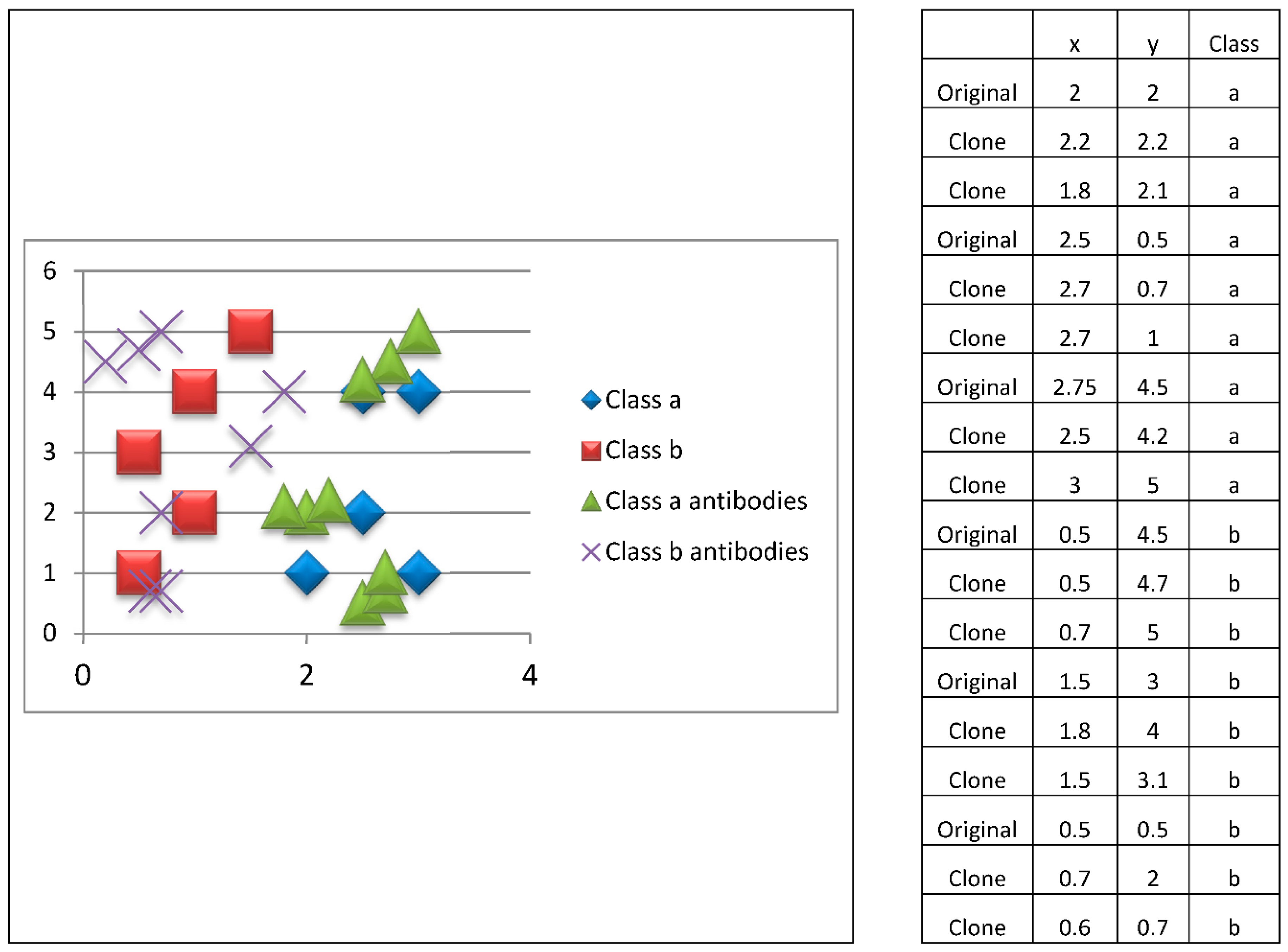
The following is an example of adaptive and innate immune responses in the proposed model. Suppose we have a training set that has 10 two-dimensional patterns, evenly distributed among two classes, as shown in Figure 4. Let us also consider that our immune system has six macrophages.
The adaptive immune response is developed as follows.
Phase 1: Detection of antigenic macromolecules
The adaptive immune response begins by determining the number of macrophages necessary to phagocyte the antigenic determinants of each antigenic macromolecule, such as:
f _ c o u n t = f   ( quantity   of   bags   ( macrophages ) ) L   ( number   of   clases   ( antigenic   macromolecules ) ) .
Thus, the macrophages are divided in such a way that they can phagocyte equitably to the antigenic determinants. Later, these antigenic determinants are presented to the T-Helper lymphocytes. In the example of Figure 4, we have two antigenic macromolecules, which correspond to two classes. Thus:
f c o u n t =   f   ( quantity   of   bags   ( macrophages ) ) L   ( number   of   clases   ( antigenic   macromolecules ) ) = 6 / 2 = 3 .
Accordingly, three bags (macrophages) will be assigned to phagocyte the antigenic determinants of each antigenic macromolecule, that is, to group the class data, through random sampling without replacement. In the example, two instances (antigenic determinants) of class a (antigenic macromolecule a) will be assigned to bag (macrophage) 1, two will be assigned to bag 2, and the remainder to bag 3. This process will be repeated for class b (antigenic macromolecule b) (Figure 5).
The initial training patterns are shown in Figure 4. We have a balanced distribution of five patterns belonging to class a, and five patterns of class b. These patterns are kept in consistent figures; however, it is important to keep in mind what the ten initial patterns are.
In Figure 5, the training patterns are grouped into equally distributed bags for each class, that is, all classes will have the same number of bags. As a consequence of the above, each class will be represented by the same number of prototypes.
Phase 2: Activation of B lymphocytes
Subsequently, each bag (macrophage) activates the corresponding merging procedure (B lymphocyte), which will release a prototype (antibody) a ¯ i corresponding to the instances (antigenic determinants) presented by the macrophage, which is determined by the mean of the instances (Figure 6).
At this stage, a unique prototype is generated with the mean value of the patterns of each bag. In this example, three prototypes are created for each class. As we can notice, there are two prototypes similar to an original training pattern; this is because in their respective bag there was only one pattern to average their values.
Phase 3: Control of the immune response
Estimation of the current prototypes’ (antibodies) ability is performed by calculating the weighted performance in order to reduce bias a little due to the possible imbalance in the data set. To do this, the instances (antigenic determinants) of the validation set are presented to the prototypes. Each prototype responds to its nearest instance (antigenic determinant).
The immune response is then adjusted so that the prototypes (antibodies) are able to correctly classify the instances (to combine with the antigenic determinants presented). To do this, the prototypes “approach” the instances of the corresponding class, and “move away” from the instances of other classes. Thus, the prototypes move in the search space, so that they obtain a better performance compared to being in their previous positions. If the new prototypes (antibodies) have a better immune response than the previous antibodies, they are replaced. This process is shown in Figure 7.
Phase 4: Development of adaptive immunity
To develop the adaptive response, the prototypes (antibodies) are cloned. This allows the algorithm to explore the search space. To achieve this, the position of the prototype is slightly modified. This process is shown in Figure 8, where two clones are generated for each prototype (antibody).
Subsequently, the antibody survival phase is performed, where a mean of the clones generated from each prototype (antibody) is obtained so that we return to the six antibodies (three from class a and three from class b). This survival process is shown in Figure 9.
If the new clones of the prototypes (antibodies) exhibit a better immune response than the previous antibodies, they are replaced. This process is iterative and elitist because it only retains the best antibodies generated. Then, these prototypes are used in the immune response. Phases 3 and 4 are repeated for a predefined number of iterations.
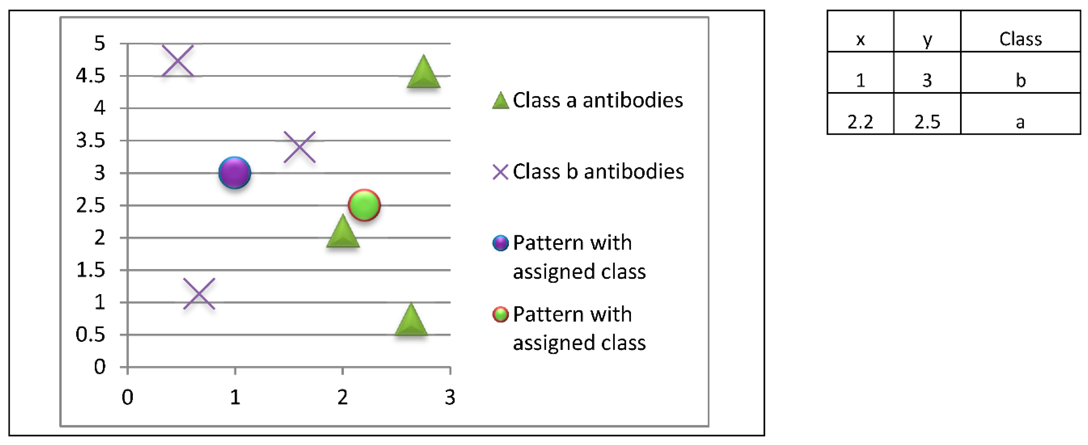
Phase 5: Threat resolution
At this stage, the final prototypes (antibodies) are stored in the immune memory (Figure 10).
Upon completion of the model construction phase (adaptive immune response), it is possible to perform the classification or model operation (innate immune response). In this case, let us suppose that we have two new patterns whose classes are unknown, as shown in Figure 11. These patterns correspond to unknown classes (antigenic determinants), and we want to respond to this threat using the prototypes (antibodies) previously stored in the immune memory.
Antibodies stored in memory will be used to classify new patterns whose class is unknown. In this example, three class a patterns and three class b patterns are stored, so each class is represented by the same number of prototypes.
The innate immune response will look for the most closely related prototypes (antibodies) to each unknown instance (antigenic determinant), so the classification would be as shown in Figure 12.
In this example, the pattern at coordinates (1.0, 3.0) would be classified as class b, while the pattern at coordinates (2.2, 2.5) would be classified as class a.
The proposed AISAC model is a contribution to the state-of-art of artificial immune systems. It provides a new modeling of the biological behavior of the immune system, and has a low computational cost. In addition, AISAC is simple and able to fit the training data using few antibodies. We consider that this model enhances the frontier of classification systems. In the next section, we test the performance of the AISAC model in a very important scenario: cancer detection.

4. Results

In this section the results obtained in this investigation are presented and discussed. First, Section 4.1 briefly describes the datasets that were used in the comparison of results. In Section 4.2, considerations related to the configuration of the parameters of the AISAC model are issued. Then, in Section 4.3 an evaluation of the running time of the proposed algorithm as well as the results of the evaluation is carried out.
Finally, in Section 4.4, the performance evaluation and the comparison of what AISAC produces with the different learning algorithms are presented and discussed.

4.1. Datasets

We decided to test the performance of the AISAC model for the cancer detection problem. We selected 10 cancer-related datasets, available from international repositories (Table 1). The datasets used were:
(a)
Breast Cancer Digital Repository (BCDR) [43]. This is a dataset of real Portuguese patients provided by the Faculty of Medicine of the University of Porto, Portugal;
(b)
Breast Cancer Wisconsin (Original) Data Set (BCWO) [44,45]. The University of Wisconsin, Madison by Dr. William H. Wolberg, provided this dataset;
(c)
Breast Cancer Wisconsin (Diagnostic) Data Set (BCWD) [45]. This dataset was created by Wolberg, Nick, and Mangasarian from the University of Wisconsin, and was donated to the UCI repository in November 1995;
(d)
Breast Cancer Wisconsin (Prognostic) Data Set (BCWP) [45]. This is a different version of the former;
(e)
Breast Cancer SEER (BCSEER) [46]. This dataset was requested to the National Cancer Institute’s Surveillance, Epidemiology, and End Results (SEER) program;
(f)
Mammographic Mass Data Set (MMDS) [47]. Matthias Elter donated this dataset to the UCI repository in October 2007. It contains patients’ age and attributes collected from digital mammograms of patients between 2003 and 2006 at the Institute of Radiology of the University Erlangen-Nuremberg;
(g)
Breast Cancer Data Set (BCDS) [45]. This dataset was provided by M. Zwitter and M. Soklic and obtained at the University Medical Centre, Institute of Oncology, Ljubljana, Yugoslavia. This dataset contains clinic data of the patients, such as age and menopause status, in addition to data corresponding to the breast tumor and recurrence;
(h)
Lung Cancer Data Set (LCDS) [45]. This dataset was published in Hong et al.’s work in 1991 and later donated by Stefan Aeberhard in May 1992. It describes three types of lung cancers;
(i)
Haberman’s Survival Data Set (HSDS) [45]. Tjen-Sien Lim donated this dataset in March 1999. It contains cases from a study of patients who had a surgery for breast cancer at the Hospital of the University of Chicago;
(j)
Thoracic Surgery Data Set (TSDS) [48]. Lubicz, Pawelczyk, Rzechonek, and Kolodziej in Wroclaw, Poland created this dataset, and Maciej Zieba and Jakub Tomczak donated it in November 2013. It contains data from patients who had lung cancer and eventually a major lung resection in the 2007 to 2011 years at the Wroclaw Thoracic Surgery Centre.

4.2. Parameter Configuration

It is well-know that swarm intelligence algorithms suffer from having many parameters to tune. Finding the appropriate values is crucial, since it can increase the performance of the algorithms. However, this is not a trivial process.
To avoid overfitting, we carried out several empirical studies of the proposed algorithm in order to determine the optimal parameters (number of iterations and the number of antigens) for each dataset.
The empirical studies allowed us to determine which parameter values were sufficient for the algorithm to obtain the best performances. Unlike the trial and error approach, empirical studies of the number of antibodies and iterations necessary for a good classification allowed us to find in a sequential way the parameters that obtained the best performance in the classification of each dataset. It is necessary to mention that the empirical studies of the number of antibodies and iterations were performed for each dataset.
Shown below is an example of a test done with the Breast Cancer Wisconsin (Prognostic) dataset (BCWP) to obtain the number of iterations and the number of antigens for the dataset.
The test for the iterations was done by using 100 antibodies and running the classification process using 100 iterations. This means that the model was tested each time and the performance after each iteration was saved. For the BCWP dataset, the results for this test are shown in Figure 13.
We can observe that the maximum performance was obtained using 30 iterations and increasing the number of iterations did not increase the performance, so 30 iterations were finally used for this dataset.
Regarding to the number of antibodies needed to obtain the better performances, we set the number of iterations at 100, and varied the number of antibodies from 2 to 100 antibodies. This means the model was tested 99 times, varying the number of antibodies in independent runs. For the BCWP dataset, the results for this test are shown in Figure 14.
We can observe that the best performance was reached using 90 antibodies; therefore, for this dataset 90 antibodies were used in classification.
In conclusion, for the BCWP dataset, 90 antibodies and 30 iterations were used. This process was repeated for each dataset individually.
Finally, in Table 2 we present the values obtained by the empirical studies for each dataset.
The values obtained show that a maximum of 100 antibodies and 90 iterations are enough for the proposed model to obtain competitive performances for classification.
This is important because 90 iterations do not represent a huge investment of time in evolutionary algorithms; likewise, representing a dataset with only 100 antibodies implies a reduction of the computational cost of classification and the cost of storing the models.
In some classification models, such as k-nearest neighbors (KNN), the training set is completely stored. This means that if the training set contains 3000 patterns, we need to store them all. In contrast, with the proposed model, we only need to store 100 antibodies for further classification.

4.3. Running Time Evaluation

Similarly, an empirical study was carried out to determine the computational cost of the algorithm, obtaining the results presented in Table 3. Table 3 refers to the running time of the algorithm in each of the datasets.
As presented in the table, the proposed algorithm obtained an average running time of 26.31 s for all datasets, with the shortest time 3.1 s and the greatest 39.4 s. It is important to highlight that less than half a minute to perform breast cancer detection is a relevant result.

4.4. Performance Evaluation

We used the five-fold stratified cross-validation (5-scv) procedure, due to the imbalance ratio of some datasets [49]. As a performance measure, we used the average classifier accuracy of the folds. The process was repeated 10 times.
This algorithm was implemented and tested in a personal computer with the following specifications: Intel Core i7 970 3.20 Ghz, 24Gb RAM memory, Windows 8.1 Pro 64bits, Hard drive 1 TB.
We tested the AISAC model in two scenarios: with respect to other immune-based learning classification systems (Section 4.4.1) and with respect to well-known learning classification systems (Section 4.4.2). In both scenarios, we used the Wilcoxon test [50] to establish the existence or lack thereof of significant differences in performance among the compared algorithms. We used a significance level of 0.1, for a 90% confidence interval. This particular statistical comparison was suggested in [51].

4.4.1. Comparison of AISAC versus Immune-Based Learning Algorithms

Table 4 shows the performance of the AISAC and other immune-based algorithms over the 10 cancer-related datasets. The best results are highlighted in bold.
When comparing the classifiers based on immune systems, we used the Wilcoxon signed rank test. This comparison is presented in Table 5. The p-Values in all cases were lower than the significant value α = 0.1 , which means that significant differences existed among the performances of AISAC and the compared algorithms within a 90% of confidence, and the null hypothesis H0 was rejected. Considering the wins, losses, and ties obtained, we can state that AISAC outperforms the other compared immune-based algorithms.
These results confirm that our proposal obtained a significantly better performance in cancer classification than all other tested immune-based learning classification systems.

4.4.2. Comparison of AISAC versus Well-Known Learning Algorithms

Table 6 shows the performance of the AISAC and other well-known learning algorithms over the 10 cancer-related datasets. The best results are highlighted in bold.
Again, we used the Wilcoxon test to compare the algorithms, and results are presented in Table 7.
These values showed significant differences for two algorithms (nearest neighbor and naïve Bayes), while there were no significant differences for the remaining five algorithms.
It is important to emphasize the breast cancer detection ability of the new model, which was significantly better than both nearest neighbor and naïve Bayes, models considered among the top 10 best algorithms in data mining. In addition, it obtained a comparable performance to the remaining ones. Although no significant differences were found, it obtained more wins than losses, and it was the best for 5 out of 10 datasets.
In 2019 [52] a preliminary work was carried out using the first version of an algorithm based on the immune system. Good results were obtained, however in this new study, analysis with a larger number of datasets and a comparison with more classification algorithms was considered. In addition, we refined the adjustment of the immune response, as well as the selection of antibodies.
Having a low computational cost while being competitive and highly configurable, this algorithm stands out as a more than adequate and novel pattern classifier.

5. Discussion

Unlike other classification algorithms, our proposal is based on a biological process, which turns our algorithm into a bio-inspired algorithm which, as presented in the results, obtains good performances compared to the rest of the classifiers.
Most datasets are imbalanced, in addition to containing missing values. The proposed algorithm is able to work with these characteristics and obtain results without significant differences against some classical classification algorithms. On the other hand, it obtained significant differences when compared to other algorithms based on the same principle; that is, our proposal surpasses those algorithms based on the same principle.
According to the statistical tests, the proposed model obtained better results compared to other algorithms, and no differences with respect to others. In no case was our proposal significantly worse than other classifiers. This opens an interesting knowledge gap about this area and its possible exploration in the use of bioinspired algorithms for classification.
The main contribution lies in the proposal of a new classification model based on the immune system obtaining good results compared to literature classification algorithms. In a similar way, the AISAC algorithm obtains good results compared to algorithms based on the same principle. The results presented reveal the possibility of using the proposed algorithm as an alternative for the classification of unbalanced datasets as well as big datasets due to their guided stochastic behavior, which allows these datasets to be classified.
To deal with the adjustment of parameters, we opted to carry out empirical studies for each dataset, obtaining the appropriate parameters for our proposed algorithm in order to make it more powerful. The analysis results presented in this work can help to explain why those parameters work well. Using these parameter values guarantees the good classification of the iterative process and it makes it possible to obtain competitive results, comparing our proposal with other classification algorithms.
We found that 100 antibodies and 90 iterations were enough to obtain accurate classification results.
Finally, in the evaluation of the running time of the algorithm it is relevant to emphasize that our algorithm does not exceed 40 s in performing the training and classification of a dataset.

6. Conclusions and Future Work

The classification model presented in this work exhibits a performance equivalent to the classic algorithms for classification, which was proven using Wilcoxon tests.
This new model is a contribution to evolutionary methods as classifiers and opens a gap for future research and developments in the area of bio-inspired classification algorithms based on the human immune system.
AISAC is not a definitive solution for classification, since there was no classifier that had the best performance for all datasets. However, notable contributions are provided to the fields of evolutionary computation, and specifically to algorithms for classification based on artificial immune systems.
The use of distributed computation can make it possible to reduce the time and computational cost of the algorithm proposed in this work; in the same way, it can allow the use of more robust algorithms for the adjustment of antibodies if the algorithm runs in parallel. However, as stated before, the computational cost of AISAC is low.
In future work we want to test with other cloning strategies, so the cloning and competition between generations can be a more extensive work that allows the development of a more robust algorithm capable of classifying imbalanced datasets with a better performance.

Author Contributions

Conceptualization, D.G.-P. and Y.V.-R.; methodology, Y.V.-R. and C.Y.-M.; software, Y.V.-R., D.G.-P. and A.J.A.-C.; validation, Y.V.-R. and O.C.-N.; formal analysis, Y.V.-R. and C.Y.-M.; investigation, A.J.A.-C., and O.C.-N.; writing—original draft preparation, Y.V.-R.; writing—review and editing, C.Y.-M.; visualization, O.C.-N. and A.J.A.-C. All authors have read and agreed to the published version of the manuscript.

Funding

This research received no external funding.

Acknowledgments

The authors gratefully acknowledge the Instituto Politécnico Nacional (Secretaría Académica, Comisión de Operación y Fomento de Actividades Académicas, Secretaría de Investigación y Posgrado, Centro de Investigación en Computación, and Centro de Innovación y Desarrollo Tecnológico en Cómputo), the Consejo Nacional de Ciencia y Tecnología (Conacyt), and Sistema Nacional de Investigadores for their economic support to develop this work.

Conflicts of Interest

The authors declare no conflict of interest.

References

  1. Zhou, X.; Wang, H.; Ding, B.; Peng, W.; Wang, R. Multi-objective evolutionary computation for topology coverage assessment problem. Knowl. Based Syst. 2019, 177, 1–10. [Google Scholar] [CrossRef]
  2. Eiben, A.E.; Smith, J. From evolutionary computation to the evolution of things. Nature 2015, 521, 476–482. [Google Scholar] [CrossRef] [PubMed]
  3. Xue, B.; Zhang, M.; Browne, W.N.; Yao, X. A survey on evolutionary computation approaches to feature selection. IEEE Trans. Evol. Comput. 2016, 20, 606–626. [Google Scholar] [CrossRef] [Green Version]
  4. Azmi, K.Z.M.; Ghani, A.S.A.; Yusof, Z.M.; Ibrahim, Z. Natural-based underwater image color enhancement through fusion of swarm-intelligence algorithm. Appl. Soft Comput. 2019, 85, 105810. [Google Scholar] [CrossRef]
  5. Wang, X.; Yang, J.; Teng, X.; Xia, W.; Jensen, R. Feature selection based on rough sets and particle swarm optimization. Pattern Recognit. Lett. 2007, 28, 459–471. [Google Scholar] [CrossRef] [Green Version]
  6. Hsieh, F.S. Decision Support for Collaboration of Carriers Based on Clustering, Swarm Intelligence and Shapley Value. Int. J. Dec. Supp. Syst. Technol. 2020, 12, 25–45. [Google Scholar] [CrossRef]
  7. Yue, Y.; Cao, L.; Hang, B.; Luo, Z. A swarm intelligence algorithm for routing recovery strategy in wireless sensor networks with mobile sink. IEEE Access 2018, 6, 67434–67445. [Google Scholar] [CrossRef]
  8. Ari, A.A.A.; Gueroui, A.; Titouna, C.; Thiare, O.; Aliouat, Z. Resource allocation scheme for 5G C-RAN: A Swarm Intelligence based approach. Comput. Netw. 2019, 165, 106957. [Google Scholar] [CrossRef]
  9. Huang, C.-L.; Dun, J.-F. A distributed PSO—SVM hybrid system with feature selection and parameter optimization. Appl. Soft Comput. 2008, 8, 1381–1391. [Google Scholar] [CrossRef]
  10. Ramirez, A.; Lopez, I.; Villuendas, Y.; Yanez, C. Evolutive improvement of parameters in an associative classifier. IEEE Lat. Am. Trans. 2015, 13, 1550–1555. [Google Scholar] [CrossRef]
  11. Chang, X.; Lilly, J.H. Evolutionary design of a fuzzy classifier from data. IEEE Trans. Syst. Mancybern. Part B 2004, 34, 1894–1906. [Google Scholar] [CrossRef] [PubMed]
  12. Kim, K. Artificial neural networks with evolutionary instance selection for financial forecasting. Expert Syst. Appl. 2006, 30, 519–526. [Google Scholar] [CrossRef]
  13. Garcia, S.; Derrac, J.; Cano, J.; Herrera, F. Prototype selection for nearest neighbor classification: Taxonomy and empirical study. IEEE Trans. Pattern Anal. Mach. Intell. 2012, 34, 417–435. [Google Scholar] [CrossRef] [PubMed]
  14. Onan, A. A stochastic gradient descent based SVM with Fuzzy-Rough feature selection and instance selection for breast cancer diagnosis. J. Med. Imaging Health Inform. 2015, 5, 1233–1239. [Google Scholar] [CrossRef]
  15. Derrac, J.; Cornelis, C.; García, S.; Herrera, F. Enhancing evolutionary instance selection algorithms by means of fuzzy rough set based feature selection. Inf. Sci. 2012, 186, 73–92. [Google Scholar] [CrossRef]
  16. Pérez-Rodríguez, J.; Arroyo-Peña, A.G.; García-Pedrajas, N. Simultaneous instance and feature selection and weighting using evolutionary computation: Proposal and study. Appl. Soft Comput. 2015, 37, 416–443. [Google Scholar] [CrossRef]
  17. Friedrichs, F.; Igel, C. Evolutionary tuning of multiple SVM parameters. Neurocomputing 2005, 64, 107–117. [Google Scholar] [CrossRef]
  18. Wolpert, D.H.; Macready, W.G. No free lunch theorems for optimization. IEEE Trans. Evol. Comput. 1997, 1, 67–82. [Google Scholar] [CrossRef] [Green Version]
  19. Dasgupta, D.; Yu, S.; Nino, F. Recent advances in artificial immune systems: Models and applications. Appl. Soft Comput. 2011, 11, 1574–1587. [Google Scholar] [CrossRef]
  20. Weng, L.; Liu, Q.; Xia, M.; Song, Y.D. Immune network-based swarm intelligence and its application to unmanned aerial vehicle (UAV) swarm coordination. Neurocomputing 2014, 125, 134–141. [Google Scholar] [CrossRef]
  21. Zhao, L.; Wang, L.; Xu, Q. Data stream classification with artificial endocrine system. Appl. Intell. 2012, 37, 390–404. [Google Scholar] [CrossRef]
  22. Ertas, G. Estimating the distributed diffusion coefficient of breast tissue in diffusion-weighted imaging using multilayer perceptrons. Soft Comput. 2019, 23, 7821–7830. [Google Scholar] [CrossRef]
  23. Cortes, C.; Vapnik, V. Support-vector networks. Mach. Learn. 1995, 20, 273–297. [Google Scholar] [CrossRef]
  24. Zhao, H.Y. The application and research of C4.5 algorithm. Appl. Mech. Mater. 2014, 513–517, 1285–1288. [Google Scholar] [CrossRef]
  25. Breiman, L. Random forests. Mach. Learn. 2001, 45, 5–32. [Google Scholar] [CrossRef] [Green Version]
  26. Watkins, A.B. AIRS: A Resource Limited Artificial Immune Classifier. Ph.D. Thesis, Mississippi State University, Starkville, MS, USA, 2001. [Google Scholar]
  27. Brownlee, J. Immunos-81, the Misunderstood Artificial Immune System; Centre for Intelligent Systems and Complex Processes (CISCP), Faculty of Information & Communication Technologies (ICT), Swinburne University of Technology (SUT): Melbourne, Australia, 2005. [Google Scholar]
  28. De Castro, L.N.; Von Zuben, F.J. Learning and optimization using the clonal selection principle. IEEE Trans. Evol. Comput. 2002, 6, 239–251. [Google Scholar] [CrossRef]
  29. Aha, D.W.; Kibler, D.; Albert, M.K. Instance-based learning algorithms. Mach. Learn. 1991, 6, 37–66. [Google Scholar] [CrossRef] [Green Version]
  30. Cohen, W.W. Fast Effective Rule Induction. In Proceedings of the Twelfth International Conference on Machine Learning, Tahoe City, CA, USA, 9–12 July 1995; pp. 115–123. [Google Scholar]
  31. John, G.H.; Langley, P. Estimating Continuous Distributions in Bayesian Classifiers. In Proceedings of the Eleventh Conference on Uncertainty in Artificial Intelligence; Morgan Kaufmann Publishers Inc.: San Francisco, CA, USA, 1995; pp. 338–345. [Google Scholar]
  32. Hall, M.; Frank, E.; Holmes, G.; Pfahringer, B.; Reutemann, P.; Witten, I.H. The WEKA data mining software: An update. ACM SIGKDD Explor. Newsl 2009, 11, 10–18. [Google Scholar] [CrossRef]
  33. Janeway, C.A.; Travers, P.; Walport, M.; Shlomchik, M.J. Immunobiology: The Immune System in Health and Disease, 5th ed.; Garland Publishing: New York, NY, USA, 2001; pp. 2–11. [Google Scholar]
  34. Abbas, A.K.; Lichtman, A.H.H.; Pillai, S. Cellular and Molecular Immunology, 9th ed.; Elsevier Health Sciences: Philadelphia, PA, USA, 2014; pp. 110–121. [Google Scholar]
  35. Reinherz, E.L.; Schlossman, S.F. The differentiation and function of human T lymphocytes. Cell 1980, 19, 821–827. [Google Scholar] [CrossRef]
  36. Farmer, J.D.; Packard, N.H.; Perelson, A.S. The immune system, adaptation, and machine learning. Phys. D Nonlinear Phenom. 1986, 22, 187–204. [Google Scholar] [CrossRef]
  37. Hunt, J.E.; Cooke, D.E. Learning using an artificial immune system. J. Netw. Comput. Appl. 1996, 19, 189–212. [Google Scholar] [CrossRef]
  38. Timmis, J.; Neal, M.; Hunt, J. An artificial immune system for data analysis. Biosystems 2000, 55, 143–150. [Google Scholar] [CrossRef]
  39. Turkoglu, I.; Kaymaz, E.D. A hybrid method based on artificial immune system and k-NN algorithm for better prediction of protein cellular localization sites. Appl. Soft Comput. 2009, 9, 497–502. [Google Scholar] [CrossRef]
  40. Dougherty, G. Pattern Recognition and Classification: An Introduction, 1st ed.; Springer Science & Business Media: New York, NY, USA, 2012; pp. 9–17. [Google Scholar]
  41. Han, J.; Pei, J.; Kamber, M. Data Mining: Concepts and Techniques, 3rd ed.; Elsevier: Cambridge, MA, USA, 2011; pp. 327–330. [Google Scholar]
  42. Dasgupta, D. Advances in artificial immune systems. IEEE Comput. Intell. Mag. 2006, 1, 40–49. [Google Scholar] [CrossRef]
  43. Moura, D.C.; López, M.A.G. An evaluation of image descriptors combined with clinical data for breast cancer diagnosis. Int. J. Comput. Assist. Radiol. Surg. 2013, 8, 561–574. [Google Scholar] [CrossRef]
  44. Mangasarian, O.L.; Wolberg, W.H. Cancer diagnosis via linear programming. University of Wisconsin-Madison. Comput. Sci. Dep. 1990, 958, 3–8. [Google Scholar]
  45. Lichman, M. UCI Machine Learning Repository. 2013. Available online: http://archive.ics.uci.edu/ml (accessed on 10 September 2019).
  46. Rajesh, K.; Anand, S. Analysis of SEER dataset for breast cancer diagnosis using C4.5 classification algorithm. Int. J. Adv. Res. Comput. Commun. Eng. 2012, 1, 72–77. [Google Scholar]
  47. Elter, M.; Schulz-Wendtland, R.; Wittenberg, T. The prediction of breast cancer biopsy outcomes using two CAD approaches that both emphasize an intelligible decision process. Med. Phys. 2007, 34, 4164–4172. [Google Scholar] [CrossRef]
  48. Zięba, M.; Tomczak, J.M.; Lubicz, M.; Świątek, J. Boosted SVM for extracting rules from imbalanced data in application to prediction of the post-operative life expectancy in the lung cancer patients. Appl. Soft Comput. 2014, 14, 99–108. [Google Scholar] [CrossRef]
  49. López, V.; Fernández, A.; Moreno-Torres, J.G.; Herrera, F. Analysis of preprocessing vs. cost-sensitive learning for imbalanced classification. Open problems on intrinsic data characteristics. Expert Syst. Appl. 2012, 39, 6585–6608. [Google Scholar]
  50. Wilcoxon, F. Individual comparisons by ranking methods. Biom. Bull. 1945, 1, 80–83. [Google Scholar] [CrossRef]
  51. Hommel, G. A stagewise rejective multiple test procedure based on a modified Bonferroni test. Biometrika 1988, 75, 383–386. [Google Scholar] [CrossRef]
  52. González-Patiño, D.; Villuendas-Rey, Y.; Argüelles-Cruz, A.J.; Karray, F. A Novel Bio-Inspired Method for Early Diagnosis of Breast Cancer through Mammographic Image Analysis. Appl. Sci. 2019, 9, 4492. [Google Scholar] [CrossRef] [Green Version]
Figure 1. Pseudocode of the adaptive immune response in the Artificial Immune System for Associative Classification (AISAC) model.
Applsci 10 00515 g001
Figure 2. Pseudocode of the adjustment in the adaptive immune response in the AISAC model.
Applsci 10 00515 g002
Figure 3. Pseudocode of the innate immune response in the AISAC model.
Applsci 10 00515 g003
Figure 4. Example of a training set containing 10 patterns (antigenic determinants), from two classes (antigenic macromolecules), a and b.
Applsci 10 00515 g004
Figure 5. Macrophages phagocytosing the corresponding antigenic determinants. Ellipses represent the macrophage.
Applsci 10 00515 g005
Figure 6. Generation of initial antibodies for each B lymphocyte.
Applsci 10 00515 g006
Figure 7. Immune response adjustment process.
Applsci 10 00515 g007
Figure 8. Cloning of antibodies.
Applsci 10 00515 g008
Figure 9. Survival of antibodies.
Applsci 10 00515 g009
Figure 10. Final antibodies in immune memory.
Applsci 10 00515 g010
Figure 11. Distribution of new antigenic determinants whose classes are unknown.
Applsci 10 00515 g011
Figure 12. Phase of resolution of the threat in the innate immune response.
Applsci 10 00515 g012
Figure 13. Iteration empirical study test results for the Breast Cancer Wisconsin (Prognostic) (BCWP) dataset.
Applsci 10 00515 g013
Figure 14. Antibodies empirical study test results for the BCWP dataset.
Applsci 10 00515 g014
Table 1. Datasets.
Table 1. Datasets.
DatasetClassesAttributesMissing ValuesImbalance Ratio
NumericCategorical
BCDR2380Yes1.06
BCDS218Yes2.36
BCWO290Yes1.9
BCSEER250No5.41
HSDS230No2.77
LCDS3560Yes1.44
MMDS250Yes1.15
TSDS2214No5.71
BCWD2300No1.68
BCWP2330Yes3.21
Table 2. Hommel values of the compared learning algorithms.
DatasetAntibodiesIterations
BCDR4030
BCDS5050
BCWO1020
BCSEER2010
HSDS4090
LCDS8020
MMDS10020
TSDS2030
BCWD3010
BCWP9030
Table 3. Average running time of the classification algorithm.
DatasetAverage Time (S)
BCDR25.1
BCDS29.1
BCWO4.7
BCSEER3.1
HSDS38.8
LCDS22.5
MMDS30.0
TSDS39.4
BCWD35.0
BCWP35.4
Table 4. Average performances obtained by the immune-based learning algorithms. The best results are highlighted in bold.
DatasetAIRS1Immunos1CLONALGAISAC
BCDR73.20456.07757.73564.360
BCWO96.71084.69294.13597.420
BCSEER94.52095.37496.513100.000
BCWD93.84990.51088.92893.670
BCWP64.14156.56674.24279.290
LCDS53.12556.25046.87568.750
MMDS63.37274.29870.03178.980
BCDS67.48373.42767.13373.776
HSDS63.72656.81073.20376.471
TSDS69.78772.97981.06485.319
Table 5. Wilcoxon test for of the immune-based algorithms.
AISAC versusWinsLossesTiespDecision
AIRS17120.035Reject H0
CLONALG10000.005Reject H0
Immunos110000.005Reject H0
Table 6. Average performances obtained by the well-known learning algorithms. The best results are highlighted in bold.
DatasetSVMMLPNNRIPPERC4.5Naïve BayesRandom ForestAISAC
BCDR80.11179.00672.92875.41474.86272.65281.49164.360
BCWO96.99695.42295.27995.56595.13695.99496.85297.420
BCSEER100.00100.0098.363100.00100.0097.153100.00100.00
BCWD97.71596.66195.95895.60693.14692.97096.83693.670
BCWP76.26376.26370.70777.77872.72766.66780.30379.290
LCDS56.25053.12553.12550.00046.87559.37543.7568.750
MMDS79.50181.16675.23482.93482.31077.83679.70878.980
BCDS69.93066.78368.18270.28074.12672.72771.32873.776
HSDS72.87672.22266.01373.85670.26174.83767.64776.471
TSDS84.46881.48975.95784.68184.46874.46884.89385.319
Table 7. Wilcoxon test for of the state of the art classification algorithms.
AISAC versusWinsLossesTiespDecision
SVM5320.673Do not reject H0
MLP6310.259Do not reject H0
NN8200.066Reject H0
RIPPER5320.779Do not reject H0
C4.56220.326Do not reject H0
Naïve Bayes9100.034Reject H0
Random Forest3430.799Do not reject H0

