Alignment Method of an Axis Based on Camera Calibration in a Rotating Optical Measurement System

Abstract

The alignment problem of a rotating optical measurement system composed of a charge-coupled device (CCD) camera and a turntable is discussed. The motion trajectory model of the optical center (or projection center in the computer vision) of a camera rotating with the rotating device is established. A method based on camera calibration with a two-dimensional target is proposed to calculate the positions of the optical center when the camera is rotated by the turntable. An auxiliary coordinate system is introduced to adjust the external parameter matrix of the camera to map the optical centers on a special fictitious plane. The center of the turntable and the distance between the optical center and the rotation center can be accurately calculated by the least square planar circle fitting method. Lastly, the coordinates of the rotation center and the optical centers are used to provide guidance for the installation of a camera in a rotation measurement system. Simulations and experiments verify the feasibility of the proposed method.

1. Introduction

In recent years, an optical measurement method based on the photogrammetry principle [1,2,3] has been developed rapidly because of its high speed, non-contact, high accuracy and flexibility. Optical measurement is one of the effective methods for coordinate measurement, trajectory measurement or surface reconstruction. It is widely used in different fields such as three-dimensional (3D) sensor measurement, panoramic image mosaic, aerospace, virtual reality (VR), augmented reality (AR), industrial manufacturing and so on [4,5,6,7,8,9].

In the large-scale scene or 360-degree annular area measurement, due to the limitation of the field of view (FOV) of the camera, a single lens camera cannot cover the whole measurement range of the target. Therefore, scanning photography [10] is employed, in which a rotating mechanism rotating around a fixed point enables the camera to enlarge the measuring range by acquiring images from multiple angles. Theoretically, adjacent images taken by the camera rotating around its projection center can be matched by a purely projective transformation of their regions of overlap without requiring the three-dimensional shape of the scene [11,12,13]. In order to facilitate calculation and later data fusion, it is crucial to coincide the optical center of the camera with the rotation center of the rotating mechanism in practice for the creation of panoramic images. Here, the optical center of the camera is the origin of the camera coordinate system in the computer vision. It is also called the projection center in many references and corresponds to the first nodal point (or principle node) of the camera lens installed in the same medium. For the close-range applications, the misalignment of the two centers will be introduced into the final results and the images may not be spliced well. For simplicity, in the rest of this article, the “optical center of the camera” is abbreviated as “optical center”.

The alignment of a rotating optical measurement system has always been a hot topic in many fields and has aroused the research interest of many researchers. Carlo Tomasi et al. [11] proposed a centering procedure, in which the rotation center was aligned by moving the camera via the translation platform with the help of the transition line of far and nearby targets, and the location accuracy can reach one tenth of a millimeter. Antero Kukko et al. [14] designed special calibration target “cones” to align the optical center with the rotation center to realize the adjustment of the digital camera to a spherical panoramic camera head. The achieved projection center uncertainty was approximated to be about 1 mm. Kauhanen et al. [15] developed a method to find the rotation center based on the camera calibration method, in which a three-dimensional calibration target is employed. The X, Y and Z shifts for the correction of the camera location were obtained by a numerical method. The standard deviation between the projection center and the rotation center after calibration could reach 0.161 mm. On the contrary, in some studies, the relationship between the camera and the rotation mechanism is calculated by the system calibration in advance, and then it is substituted into the final image mosaic [16,17,18]. For instance, Zhang Zuxun et al. [19,20] designed a measuring system named Photo Total Station System (PTSS), within which a metric camera with known internal parameters was rigidly installed on the telescope of the total station to extend the FOV and improve the accuracy. Zhang et al. [21] designed a theodolite–camera (TC) measurement system consisting of a theodolite and a camera for precise measurement at large viewing angles. The total station or theodolite can provide the spatial coordinates of the control points, which can be used to establish the relationship of the camera while rotating. This kind of measurement system needs a complicated calculation process to eliminate the influence of the misalignment between the optical center and the rotation center.

For any rotating optical measurement system, the motion trajectory of the optical center will be a circle centered on the rotation center. If the radius of the circle is equal to 0, it means that the optical center coincides with the rotation center. Otherwise, the optical center is not matched with the rotation center. However, since the imaging system is composed of multiple lenses, it is hard to accurately calculate and determine the real position of the optical center. Therefore, it is a challenge to guarantee a good alignment between the optical center and the rotation center, and any misalignment could affect the subsequent information stitching.

In order to calculate the coordinates of the optical center and rotation center to solve the alignment problem, the idea of camera calibration [22,23,24,25,26] is introduced. In this paper, we propose a method based on Zhang’s camera calibration principle [27] to calculate the positions of the optical center in a unified world coordinate system from the external parameters (including translation vector and rotation matrix) of the camera in a rotating optical measurement system composed of a non-metric camera and a general rotating platform. With the rotation of the turntable, a set of external parameter matrices are obtained, from which a series of optical centers can be calculated to find out the rotation center by the least square circle (LSC) fitting method. The optical center and the rotation center provide the guidance for installation of the camera in a rotating measurement system. In order to reduce the fitting complexity and improve the fitting accuracy, we introduce an auxiliary plane coordinate system to map the optical centers on a unified virtual plane before circle fitting. In addition, for reducing the errors, we collect the images when the camera rotates from different positions, and multiple sets of optical centers are calculated simultaneously to obtain multiple fitted circle centers. The weighted algorithm is used to determine the final rotation center. Computer simulations and some experiments verify that the method can guide the installation and adjustment of the rotating optical measurement system.

The rest of the paper is organized as follows: Section 2 illustrates the principle of the proposed method. Section 3 shows some simulations to validate the proposed method. Section 4 displays some experimental results to validate the proposed method and discusses the strengths and contributions of the proposed method. Section 5 summarizes this paper.

2. Principle

In this section, we explain the basic composition of the proposed rotating optical measurement system and the related techniques for finding out the rotation center.

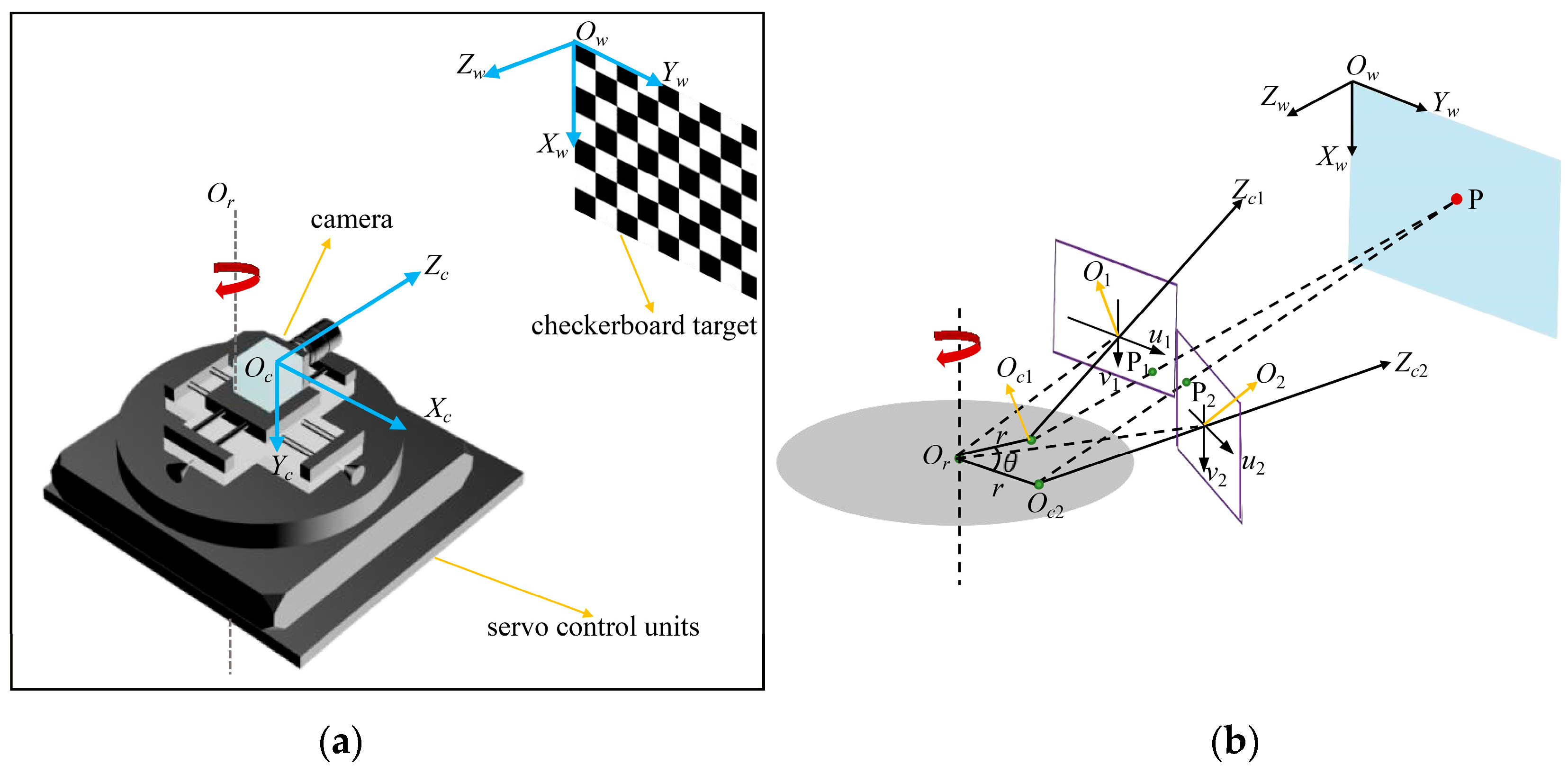
2.1. The Composition of the Rotating Optical Measurement System

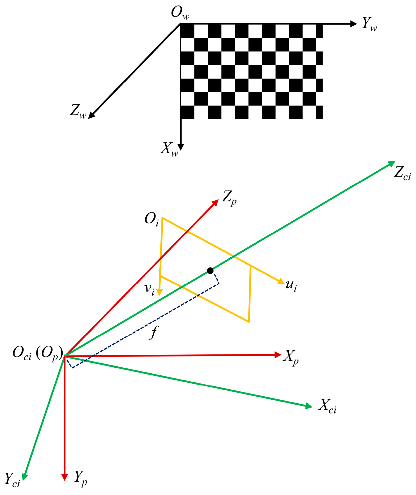
The established rotating optical measurement system and the calibration unit include a checkerboard target, a camera, servo control units, computer processing units, etc. The schematic diagram of the measurement system is shown in Figure 1a.

In Figure 1a, the camera is placed on the servo control units composing of a rotating platform and two translation platforms perpendicular to each other. The two translation platforms are fixed on the turntable to move the camera for multiple calibrations and final alignment. O_r is the rotation axis of the turntable. O_c-X_cY_cZ_c is the camera coordinate system, and O_w-X_wY_wZ_w is the fixed world coordinate system. We will give the explanations about these coordinate systems in Section 2.2. The checkerboard target is fixed in front of the system for camera calibration. A sequence of the images, which include the whole checkerboard or a part of the checkerboard, will be collected while the camera is rotated by the turntable.

2.2. Imaging Model

First, we give an introduction about the imaging model of the rotating optical measurement system. As shown in Figure 1b, O_r is the rotating axis, P is a point on the target, and P₁ and P₂ are its imaging points when the camera is rotated to Position 1 and Position 2. O_c1 and O_c2 are the optical centers for the two shots, respectively. $\overline{O_c{}_1{Z}_{c1}}$ and $\overline{O_c{}_2{Z}_{c2}}$ are the optical axis directions of the camera, O_i-u_iv_i (i = 1, 2) are the image coordinate systems, and the origin is O_i. The rotating angle between $\overline{O_r{O}_c{}_1}$ and $\overline{O_r{O}_c{}_2}$ is θ; that is, ∠O_c1O_rO_c2 = ∠O₁O_rO₂ = θ. $\overline{O_c{}_1{O}_1}=\overline{O_c{}_2{O}_1}=f$, where f is the focal length of the camera. If the optical center deviates from the rotation axis of the turntable, O_c1 and O_c2 should be on a circle centered on the rotation center; that is, $\overline{O_r{O}_c{}_1}=\overline{O_r{O}_c{}_2}=r$, where r is the radius of the circle. When the optical center coincides with the rotation center, r→0. The positions of the rotation center and optical centers can be obtained with our method. They can be used to guide the alignment of the optical center and rotation center by adjusting the distance and direction of the camera movement. The details will be presented in the next sections.

Theoretically, the sequential positions of the optical centers should be located at the whole circle as evenly as possible when the camera is rotated by the turntable. However, the obtained positions could only be located at a small arc of the circle, because it is almost impossible to provide a very large and circular calibration target. In order to improve the calculation accuracy of the rotation center, the camera is moved to different positions to collect multiple groups of images to obtain multiple sets of optical centers. Only if the turntable plane is parallel to the plane O_w-Y_wZ_w and the optical axis of the camera is perpendicular to the target at each initial position, the motion trajectory of the optical center is on the concentric circular arc parallel to O_w-Y_wZ_w. However, for an actual rotating optical measurement system, the above conditions may not be met in the calibration process, which makes the obtained fitted circles not concentric. For overcoming the problem, we introduced an auxiliary coordinate system, O_p-X_pY_pZ_p. The relationship between O_p-X_pY_pZ_p and O_w-X_wY_wZ_w is depicted in Figure 2. The auxiliary coordinate system helps us map the multiple sets of optical centers to the plane parallel to O_w-Y_wZ_w to find out the rotation center by fitting planar concentric circles.

Here, we emphasize the four coordinate systems used in the calibration for clarity.

• World Coordinate System O_w-X_wY_wZ_w is a right-handed (X_w-Y_w-Z_w), orthogonal, three-dimensional coordinate system, whose original point O_w is established on the upper left corner of the fixed checkerboard plane; that is, Z_w = 0 for points on the fixed checkerboard plane. The world coordinate system is selected as reference coordinate system during calibration.
• Image Coordinate System O_i-u_iv_i is an orthogonal coordinate system fixed in the image plane of the camera, where the u_i and v_i axes are parallel to the upper and side edges of the sensor array, respectively, and the origin O_i is located at the upper left corner of the array.
• Camera Coordinate System O_ci-X_ciY_ciZ_ci is a right-handed (X_ci-Y_ci-Z_ci), orthogonal coordinate system. The origin O_ci is located at the camera’s optical center, and the Z_ci axis is perpendicular to the image plane and coincides with the optical axis of the camera. The X_ci and Y_ci axes are parallel to the u_i and v_i axes of the O_i-u_iv_i, respectively. The plane where Z_ci = f is the image plane, where f is the principal distance between the optical center and the image plane.
• Auxiliary Coordinate System O_p-X_pY_pZ_p is a right-handed (X_p-Y_p-Z_p), orthogonal coordinate system. Its origin O_p is located at the optical center. The plane X_pO_pZ_p is a virtual plane, whose axis of X_p and Y_p are parallel to that of Y_w and X_w in the same direction, respectively, and the axis of Z_p is parallel to that of Z_w in the opposite direction.

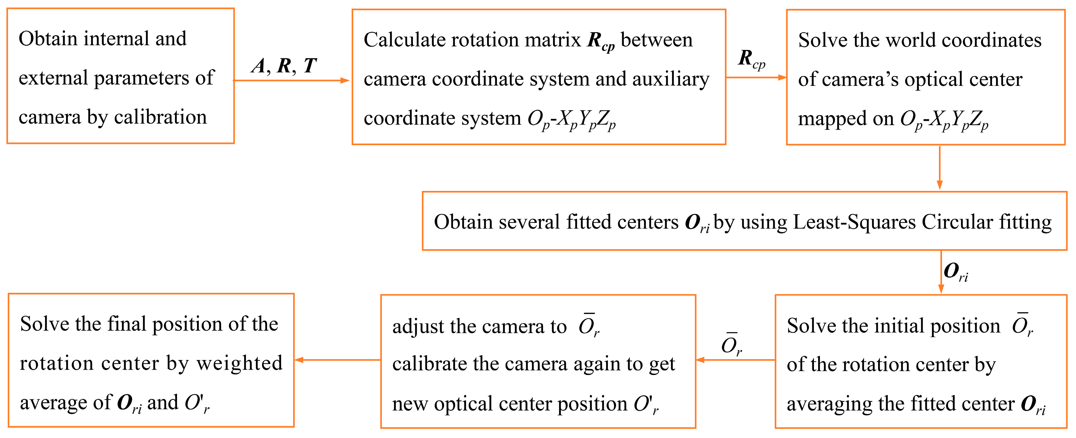
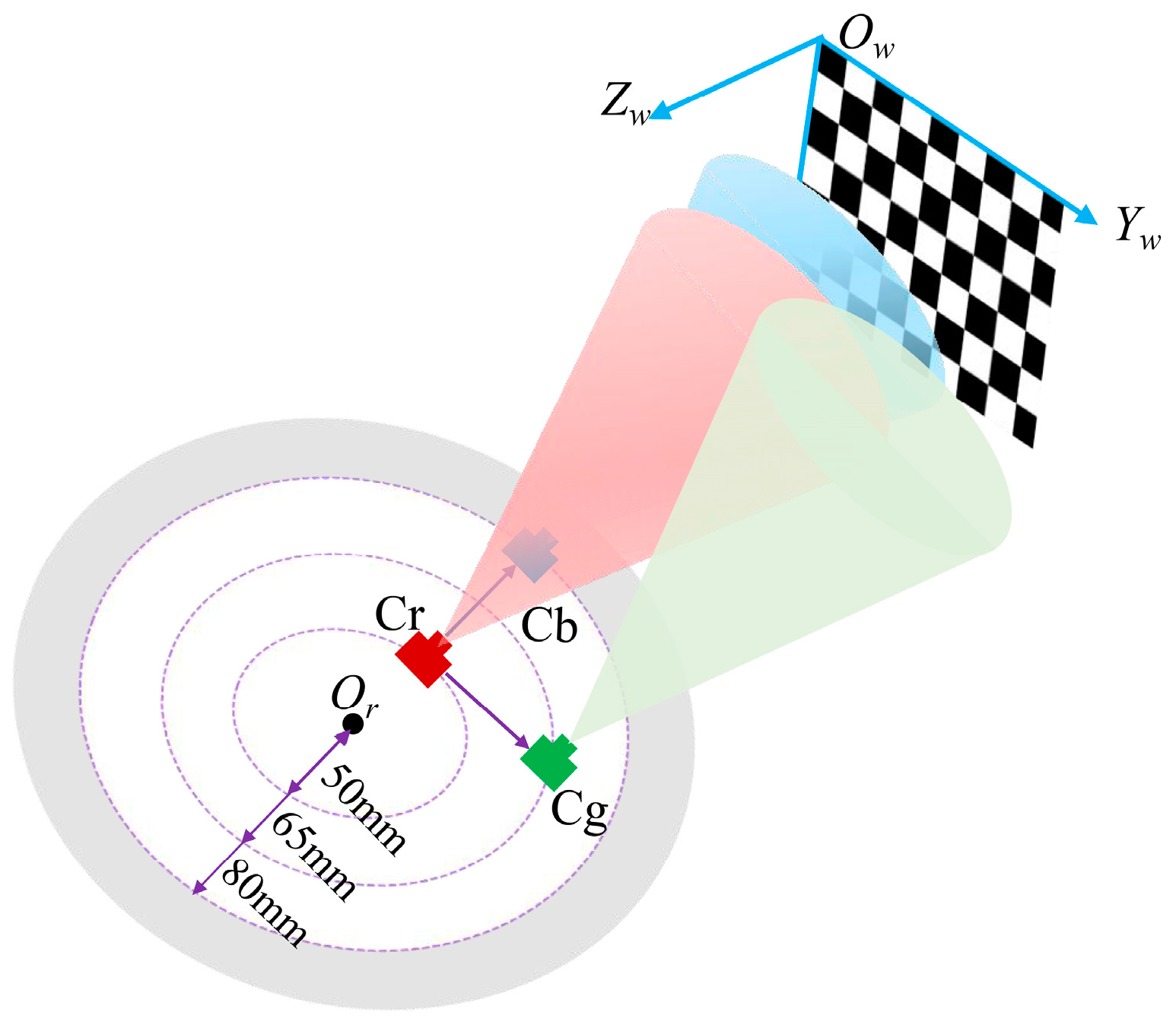
2.3. Steps to Determine the Rotation Center of the Rotating Optical Measurement System

The procedure for determining the rotation center of the rotating optical measurement system is divided into three steps. First, we collect images when the camera rotates from different positions (i) and calibrate the internal parameters and external parameters (rotation matrix R and translation vector T) of the camera by Zhang’s method. Then we can get the coordinates of the optical centers in the unified world coordinate system. Second, with the help of the auxiliary coordinate system, we calculate the rotation center by the LSC fitting method from the obtained world coordinates of the optical centers. At last, the final rotation center is obtained through a weighted algorithm. The flow chart of the procedure is shown in Figure 3.

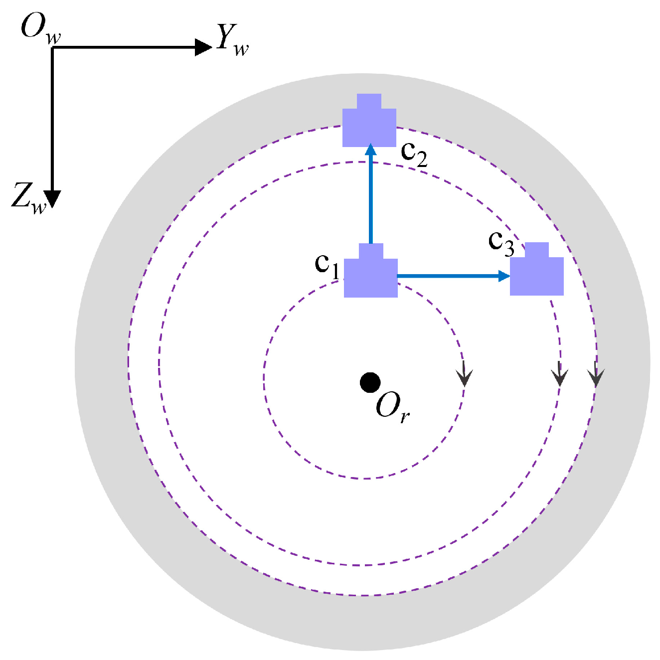
2.3.1. Calculate the Optical Center of the Camera

In the traditional camera calibration method based on the pinhole camera model, the camera’s internal and external parameters are calculated from feature points with known world coordinates and corresponding image coordinates. The relationship between the camera coordinate system and world coordinate system is described by the rotation matrix R and translation vector T. R and T reflect the spatial position of the camera in the fixed world coordinate system. If the homogeneous coordinates of the points in the world coordinate system M = (X_w, Y_w, Z_w, 1)^T and their image coordinates m = (u, v, 1)^T are known, the relationship between M = (X_w, Y_w, Z_w, 1)^T and m = (u, v, 1)^T is described as

$$s\left[\begin{array}{c}u\\ v\\ 1\end{array}\right]=\left[\begin{array}{cccc}{f}_x& \alpha & u_0& 0\\ 0& f_y& v_0& 0\\ 0& 0& 1& 0\end{array}\right]\left[\begin{array}{cc}\mathit{R}& \mathit{T}\\ 0^{\mathrm{T}}& 1\end{array}\right]\left[\begin{array}{l}{X}_w\\ Y_w\\ Z_w\\ 1\end{array}\right]=\mathit{A}\left[\begin{array}{cc}\mathit{R}& \mathit{T}\\ 0^{\mathrm{T}}& 1\end{array}\right]\left[\begin{array}{l}{X}_w\\ Y_w\\ Z_w\\ 1\end{array}\right],$$

(1)

where s is an arbitrary non-zero scale factor; f_x and f_y are scale factors of the u-axis and v-axis, respectively; α is the skew factor of two image axes; and (u₀, v₀) is the principal point of the camera. Rotation matrix R is an orthogonal unit matrix, T is a three-dimensional translation vector, and A is the internal parameter matrix of the camera, defined as

$$\mathit{A}=\left[\begin{array}{cccc}{f}_x& \alpha & u_0& 0\\ 0& f_y& v_0& 0\\ 0& 0& 1& 0\end{array}\right].$$

(2)

In Zhang’s method [27], the target plane is located on the X_wO_wY_w plane of the world coordinate system, where Z_w = 0. Equation (1) is simplified as Equation (3),

$$sm=\mathit{H}M,$$

(3)

where H = [h₁ h₂ h₃] = λA [r₁ r₂ t] is a 3×3 matrix and λ is a constant. The homography matrix H sets up the mapping between the points on the target with the points on the image. Multiple target images with different poses (at least two in theory) are needed to calculate the internal and external parameters of the camera.

In our calibration, for providing the fixed reference world coordinate system, we keep the target still and rotate the camera to calibrate R and T. Assuming the coordinates of a point are M_c in the camera coordinate system and M_w in the world coordinate system, the relationship between M_c and M_w is connected by the following rigid motion equation:

$$M_c=\mathit{R}{M}_w+\mathit{T}.$$

(4)

If M_c is known, M_w can be obtained by Equation (5):

$$M_w={\mathit{R}}^{-1}(M_c-\mathit{T}).$$

(5)

Since the rotation matrix R is an orthogonal unit matrix, R^T = R⁻¹, Equation (5) can be rewritten as

$$M_w = {\mathit{R}}^{\mathrm{T}}(M_c-\mathit{T}).$$

(6)

The coordinates (0, 0, 0) of the optical center in camera coordinate system can be mapped to the world coordinate system by Equation (6). The motion trajectory of the optical centers should be a circular arc on the turntable plane when the camera is rotated by the turntable. In practice, with the help of auxiliary coordinate system O_p-X_pY_pZ_p, Equation (7) is needed to map the optical centers on the plane parallel to O_w-Y_wZ_w,

$$M_w={\mathit{R}}_{cp}{\mathit{R}}^{\mathrm{T}}(M_c-\mathit{T}),$$

(7)

where R_cp is a 3×3 rotation matrix, which describes the rotation relationship between the camera coordinate system and auxiliary coordinate system.

2.3.2. Method for Coincidence of the Optical Center and the Rotation Center

Since not enough of the optical centers can be obtained when the camera is rotating at one position, the camera is moved to different positions to collect more images, as shown in Figure 4, where c_i (i = 1, 2, 3) represent the three initial positions of the camera. In order to easily move the camera through the translations to align the rotation center, we need c₁c₂⊥c₁c₃, c₁c₂∥O_wZ_w, c₁c₃∥O_wY_w.

The LSC fitting [28] is performed to calculate the rotation center, which satisfies that the sum of the squares of the distances between each sample point and the fitting curve must be minimized. Let (y₀, z₀) be the two-dimensional (2D) coordinates of the rotation center and (y_j, z_j) (j = 1~N, N is the number of camera rotation) be the 2D coordinates of the optical centers projected onto the Y_wO_wZ_w plane. In order to obtain (y₀, z₀), the objective function is

$$C=\min {\displaystyle \sum _{j=1}^N[{(y_j-y_0)}^2+{(z_j-z_0)}^2-R^2]}.$$

(8)

Theoretically, the radius of the fitted circle varies when the camera is moved, but the circle centers should remain unchanged. However, there are deviations among the fitted centers O_ri in the actual fitting. The initial rotation center O_r is decided by the average of the O_ri. We adjust the camera to O_r and calibrate the camera again to get a set of new optical centers O’_rj, whose average is O’_r. The weighted average value of O_ri and O’_r is taken as the final rotation center O_r = (O_y, O_z). The calculation formula is as follows:

$$O_y={\displaystyle \sum _{m=1}^{n+1}{k}_{ym}{O}_{ym}},$$

(9)

$$O_z={\displaystyle \sum _{m=1}^{n+1}{k}_{zm}{O}_{zm}},$$

(10)

where O_ym and O_zm represent the coordinates of the fitted circle centers O_ri and O’_r in the Y_w and Z_w directions, respectively; m = 1, 2, … n+1, where n is the number of the fitted circles. k_ym and k_zm represent the weighted factors, respectively, which are decided by the variance σ_m = (σ_ym, σ_zm) of each group of the optical centers by Equations (11) and (12),

$$k_{ym}=\frac{{\sigma }_{ym}}{{\displaystyle \sum _{m=1}^{n+1}{\sigma }_{ym}}},$$

(11)

$$k_{zm}=\frac{{\sigma }_{zm}}{{\displaystyle \sum _{m=1}^{n+1}{\sigma }_{zm}}}.$$

(12)

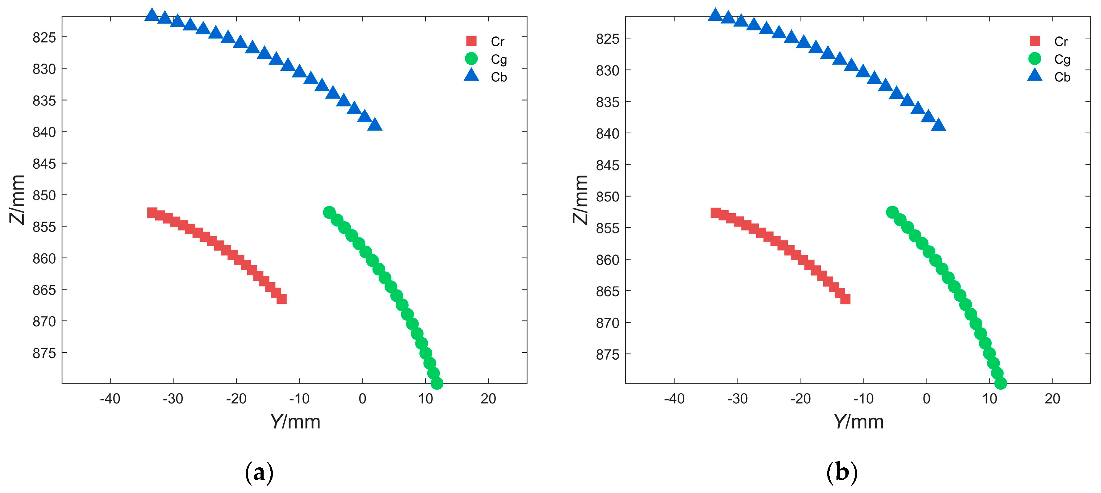
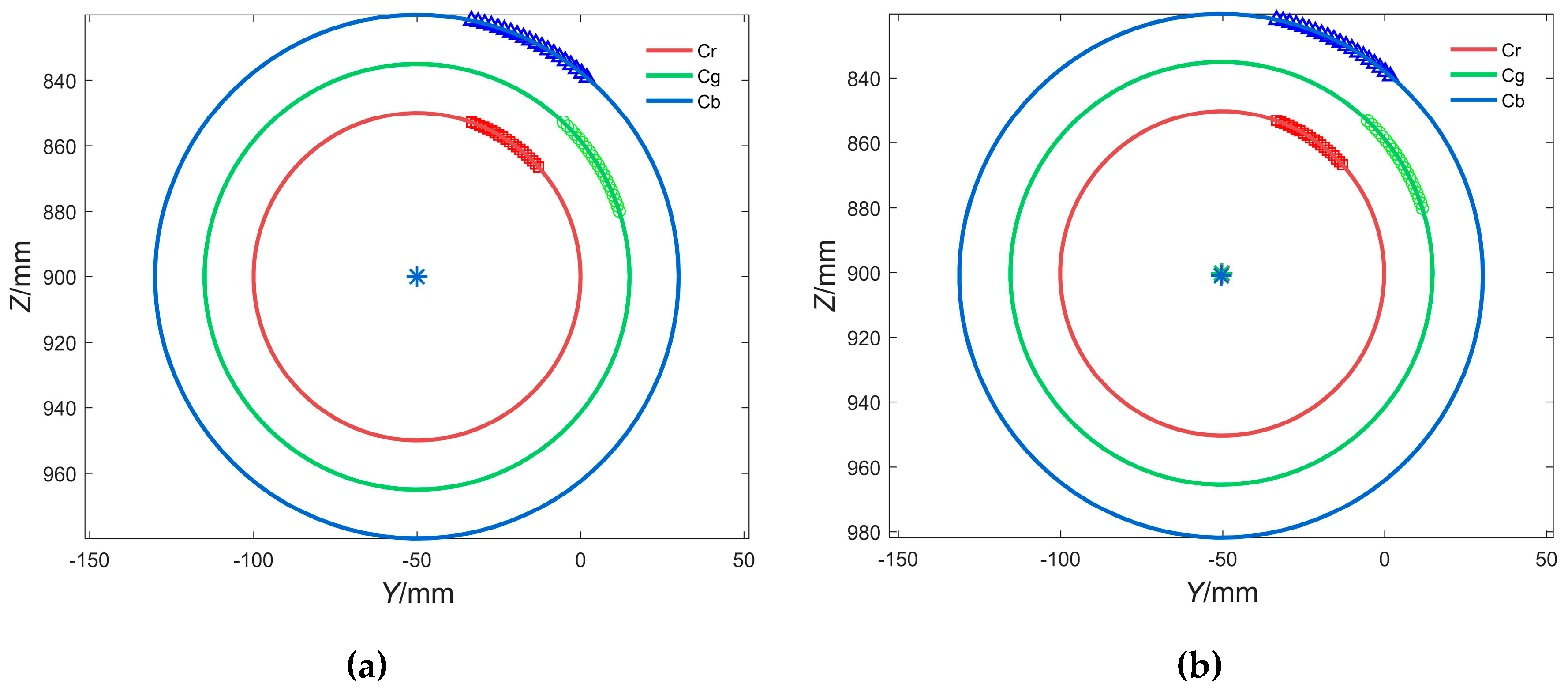
3. Computer Simulation

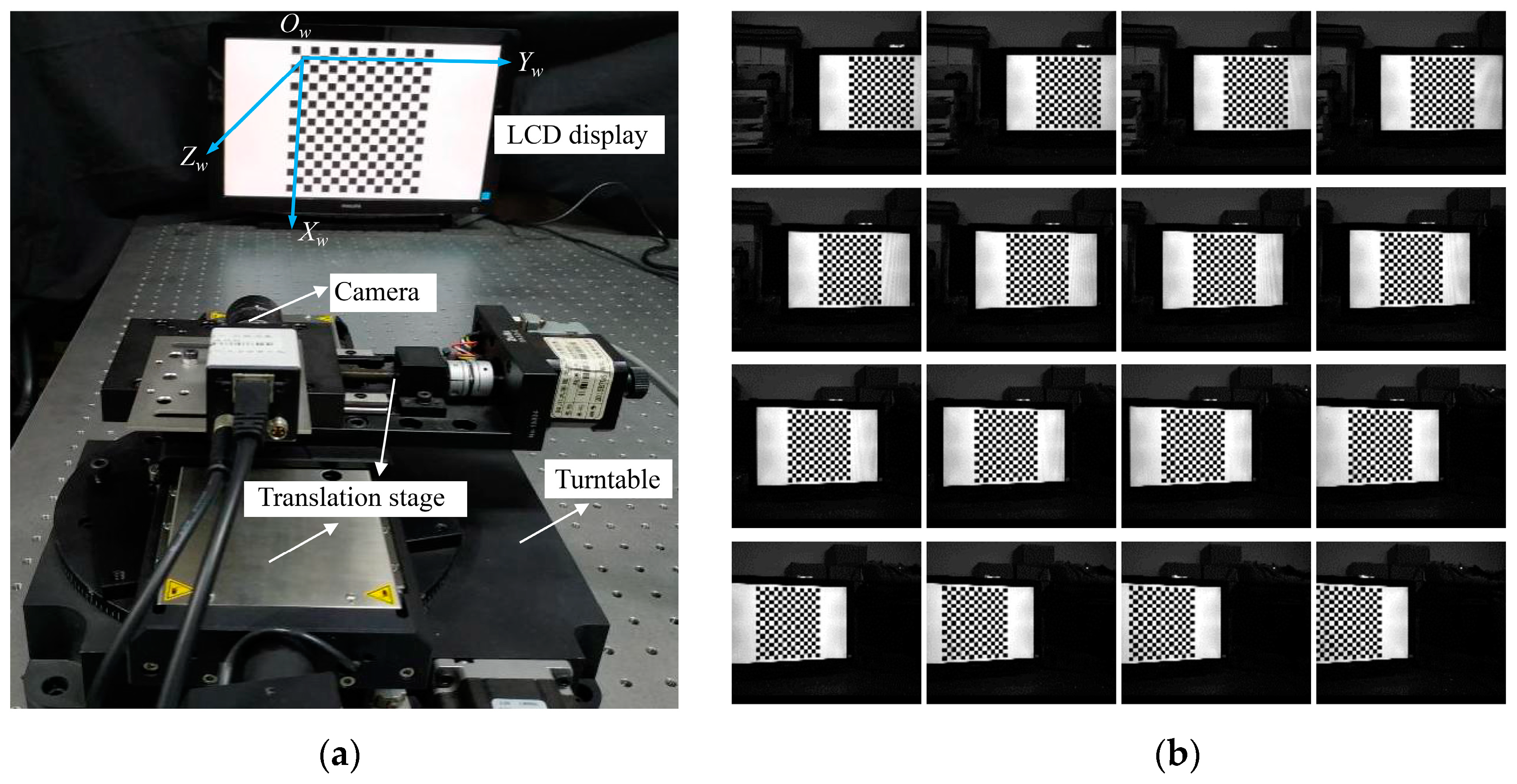
In order to verify our method, we carried out computer simulations. The simulated camera had the following parameters: f_x = f_y = 1700.00 pixels, u₀ = 600.00 pixels, v₀ = 500.00 pixels and α = 0. The size of a square of the simulated checkerboard is 14.175 × 14.175 mm. The simulated rotation center in the world coordinate system is O_r = (−80.00, −50.00, 900.00) mm. The simulated camera is placed at Cr = (−80.00, −33.31, 852.87) mm, Cg = (−80.00, −5.26, 852.85) mm and Cb = (−80.00, −33.37, 821.75) mm in the world coordinate system and 50.00 mm, 65.00 mm and 80.00 mm away from the rotation center, respectively, as shown in Figure 5.

For each position, 20 pairs of external parameter matrices (R and T) were assigned to simulate the movement of the camera. A total of 60 simulated images “seen” by the camera were substituted into Zhang’s method to calculate the internal parameters A and external parameters R and T, from which the positions of the optical centers were obtained. Then 3.5% Gaussian noise was added to affect the coordinates of each pixel of the images; the same operation is performed to calculate A, R and T and the optical centers. The obtained internal parameters in both cases are shown in

Table 1. Simulated calibration results.

Parameter	fx/Pixels	fy/Pixels	u0/Pixels	v0/Pixels	α	Pixel Error/Pixels
Without noise	1700.00	1700.00	600.00	500.00	0	0
3.5% Gaussian noise	1698.84	1698.78	599.77	500.05	0	0.035

. The trajectories of the three groups of the optical centers projected on the Y_wO_wZ_w plane are shown in Figure 6. Figure 6a is the result without noise, and Figure 6b is the result with noise. The fitted circle curves by the LSC fitting method are shown in Figure 7. The fitted centers and radii are shown in

Table 2. Fitted centers and radii correspondence table.

	Fitted Center/mm	Fitted Radius/mm
Without noise	Or = (−50.00, 900.00)	r = 50.00
	Og = (−50.00, 900.00)	r = 65.00
	Ob = (−50.00, 900.00)	r = 80.00
3.5% random noise	Or = (−49.96, 900.04)	r = 49.96
	Og = (−50.01, 900.03)	r = 65.19
	Ob = (−49.96, 900.01)	r = 79.99

.

It can be seen from Table 2 that the three circle centers and radii are the same as the setting values without considering noise. When there is 3.5% Gaussian noise, the average of the three circle centers is O_r = (−49.98, 900.02) mm, and the errors of the fitted center and radius are less than 0.05 mm and 0.19 mm, respectively. These results confirm that the proposed method can be used to locate the rotation center in the rotating optical measurement system.

4. Experiment

4.1. Experimental Setting

We carried out experiments to verify our method. The experimental setup is shown in Figure 8a. The rotation control system is composed of a CCD camera (model: Bammer camera TXG50; resolution: 1224 × 1025 pixels) with a 16 mm focus length imaging lens (model: MA1214M-MP), two translation stages (Zolix TSA50-C electric translation platform, with a repositioning precision less than 5 μm; PI-M406, with a repositioning precision of 0.078 μm) and a turntable (Zolix RAP200 electric rotation platform, with a repositioning precision less than 0.005°). The translation stages are fixed on the rotation platform, and the camera is fixed on a translation stage. The stepper motor controls the camera to move along the Y_w and Z_w axes and rotate with the turntable, respectively. During the experiment, the exposure time of the camera is 12,000 μs. The checkerboard image (the size of a square is 14.175 × 14.175 mm) is displayed on an LCD screen (Philips 190V with a resolution of 1440 × 900 pixels; the dot pitch is 0.2835 mm/pixel). The LCD display screen keeps still during the calibration process. Since the LCD display has a completely pure plane and the screen glass is very thin, the refraction phenomenon can be ignored. Of course, a checkerboard target with a higher machining accuracy can also be employed for providing feature points with higher accuracy.

4.2. Determination of the Rotation Center

In the experiment, the camera is respectively placed at three different positions, as shown in Figure 4, where c₁c₂⊥c₁c₃, c₁c₂ = c₁c₃ = 20 mm. At each initial position, the camera is rotated 16 times, for a total of 22.5 degrees with 1.5 degrees per step. Therefore, in total, 48 frame patterns will be captured during the rotation of the turntable and divided into three sets. One set of the patterns is shown in Figure 8b. The screen is placed within the depth of field of the camera lens to avoid the influence of the defocus on the calibration results. The external parameter matrices (R and T) are obtained by Zhang’s method, in which the calculated R and T are almost lens-distortion-free. The re-projective pixel error of the calibration results was 0.039 pixels in our experiment.

From the rotation matrices obtained by the calibration, the rotation angles γ_ix(j), γ_iy(j) and γ_iz(j) (i = 1, 2, 3, j = 1, 2, ..., 16) of the X_w, Y_w and Z_w axes of the world coordinate system with respect to the X_c, Y_c and Z_c axes of the camera coordinate system of the initial position can be calculated, respectively. Theoretically, if the optical axis Z_c of the camera at initial position is parallel to Z_w and the plane O_c-X_cZ_c is parallel to the plane O_w-Y_wZ_w, the rotation angle γ_iy(j) should be equal to the actual rotation angle of the turntable, and the rotation angle γ_ix(j), γ_iz(j) = 0 when the camera is rotated around the Y_c axis, as shown in Figure 9a. Three sets of the angle curves are marked with a different color in the figure, where the horizontal axis represents the times of the camera’s rotation, which is marked as N = 16(i − 1) + 1~16i. In fact, the rotation angles γ_ix(j) and γ_iz(j) fluctuate around 0 degree. We use γ’_ix(j), γ’_iz(j) and γ’_iy(j) to express the calculated three rotation angles, respectively, as shown in Figure 9b. If the three angles are used to calculate the optical centers directly, the three fitted centers will not be concentric on the plane O_w-Y_wZ_w. Figure 10a,b shows the projection of optical centers on the plane O_w-Y_wZ_w and the fitted trajectory, respectively. The deviations of the circle centers are large, by which the rotation center can not be found accurately. With the help of the auxiliary coordinate system O_p-X_pY_pZ_p, the optical centers can be mapped on a plane parallel to O_w-Y_wZ_w through the rotation matrix R_cp. In R_cp, the three rotation angles are Δγ_ix(j) = γ’_ix(j) − γ_ix(j), Δγ_iy(j) = γ’_iy(j) − γ_iy(j) and Δγ_iz(j) = γ’_iz(j) − γ_iz(j). After the angle correction with R_cp, the optical centers calculated by Equation (7) are unified to the same world coordinate system.

Three sets of the optical centers and the fitted circular arcs with different radii on the O_w-Y_wZ_w plane are shown in Figure 11a,b. Employing the optical center coordinates, the distance among c₁, c₂ and c₃ are calculated, c₁c₂ = 20.16 mm and c₁c₃ = 20.08 mm. The errors of the distance are 0.78% and 0.42%, respectively. The fitting results and the root mean square error (RMSE) of the three groups are displayed in

Table 3. Fitting results.

The Initial Position of the Camera	Fitted Center/mm	Fitted Radius/mm	RMSE/mm
c1	Or1 = (−55.23, 961.58)	r1 = 71.62	0.042
c2	Or2 = (−55.38, 961.88)	r2 = 53.32	0.054
c3	Or3 = (−55.00, 961.53)	r3 = 67.29	0.042

. The average value of the three fitted centers is O_r = (−55.20, 961.67) mm, which is regarded as the initial value of the rotation center.

In order to obtain a more accurate rotation center, we adjusted the camera to O_r, employing the translation stages along the Y_w and Z_w directions, respectively, and rotated the camera 16 times to calculate the optical centers O’_rj, which are distributed over a small range, as shown in Figure 12. The average value of O’_rj is O’_r = (−54.59, 962.05) mm. The final rotation center O_r is calculated by employing O_r1, O_r2, O_r3 and O’_r using Equations (9)–(12), where O_r = (−54.69, 961.96) mm. The camera is moved to O_r and rotated 16 times to calculate the optical centers O’’_rj. The standard deviation (STD) of O’_rj relative to O_r and O’’_rj relative to O_r in the Y_w and Z_w directions are shown in

Table 4. The standard deviation in the Y_w and Z_w directions.

Standard Deviation/mm	Yw	Zw
O’rj relative to Or	0.029	0.141
O’’rj relative to Or	0.022	0.117

. It is obvious that O_r is more reliable than O_r. These results indicate that the camera’s optical center has been positioned accurately with the rotation center of the turntable and the systematic uncertainty in our method remains about 0.1 mm.

4.3. Verification

Two experiments are designed to prove whether the optical center is aligned with the rotation center by our method after the camera has fixed the position O_r.

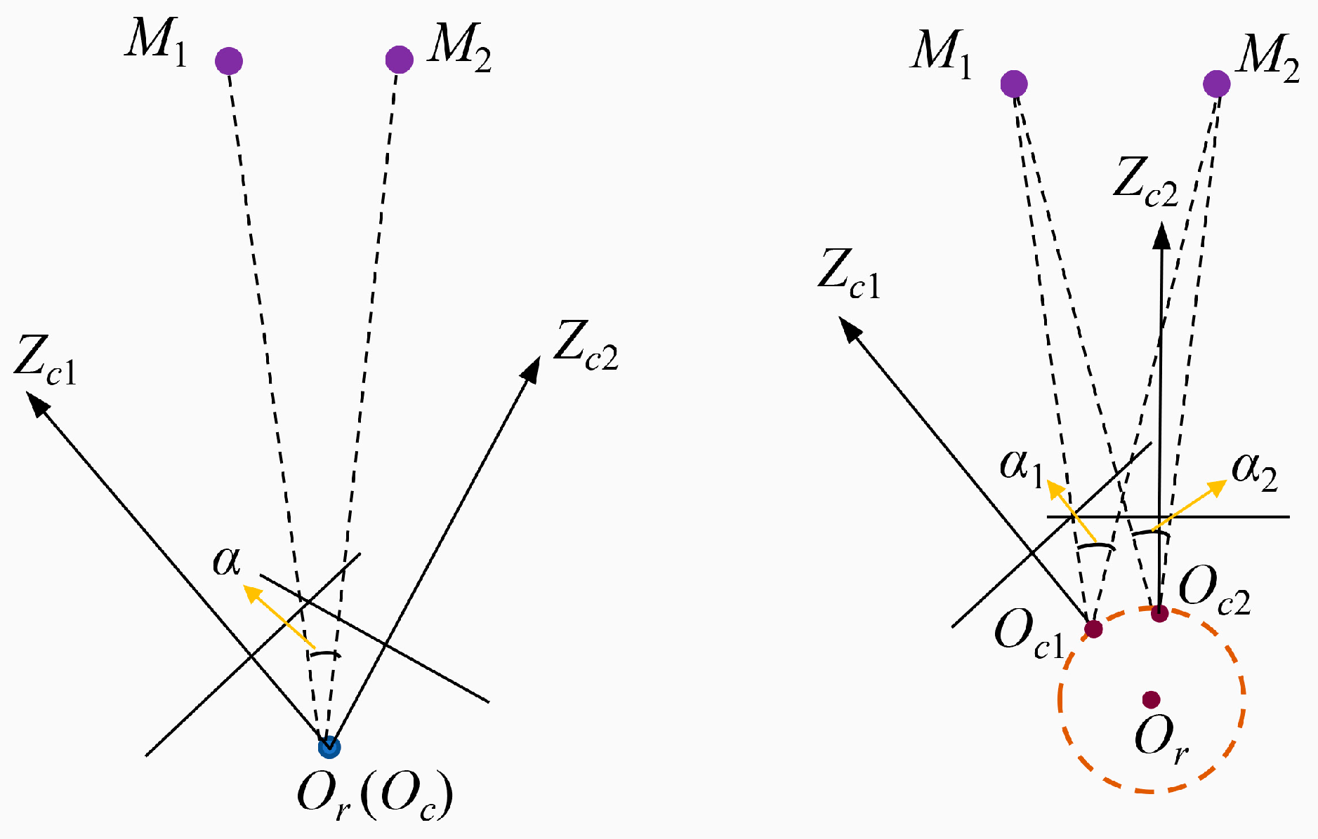
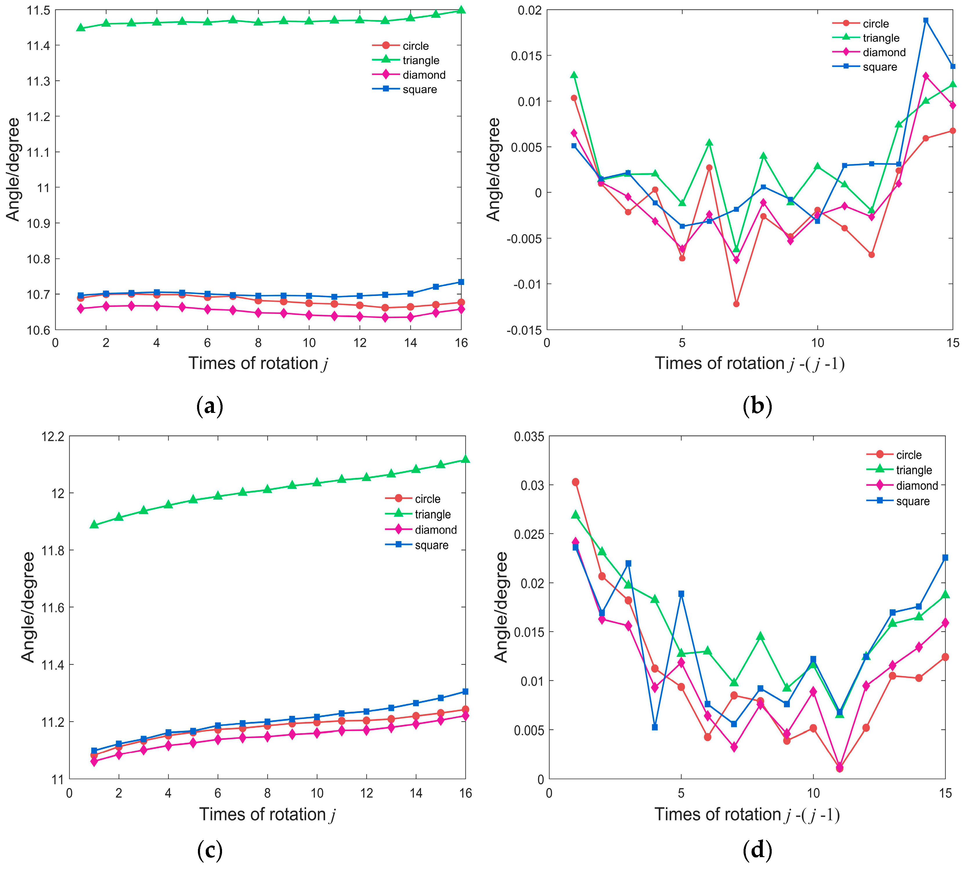
4.3.1. Calculating the Angle Formed by the Two Space Points M₁, M₂ and the Optical Center

In the experiment, we calculated the angle α formed by the two space points M₁, M₂ and the optical center, as shown in Figure 13. When the optical center coincides with the rotation center, the angle α shall remain unchangeable when the camera is rotated. However, when the optical center does not coincide with the rotation center, the angle will change with the rotation of the camera on the turntable; that is, α₁ ≠ α₂.

In the experiment, the four points pairs with different positions on the checkerboard plane are selected to calculate the angle α_k (k = 1~4) and marked as a red circle, green triangle, pink diamond and blue square, as shown in Figure 14. Sixteen angles α_k (j) (j = 1, 2, …, 16) are calculated when camera is rotated under the condition of the coaxial; the four angle curves are shown in Figure 15a and the four difference curves of the adjacent angles are shown in Figure 15b. We moved the camera away from the rotation center; the calculated angle curves are shown in Figure 15c and the four difference curves of the adjacent angles are shown in Figure 15d. The standard deviation of the four sets of angles in both cases are shown in

Table 5. The standard deviation of the angles of the four sets of marker points.

Standard Deviation/Degree	Red Circle	Green Triangle	Pink Diamond	Blue Square
Alignment	0.013	0.011	0.011	0.011
Misalignment	0.043	0.066	0.043	0.057

. It can be seen from Figure 15 and Table 5 that the angles α_k of the four groups of marker points in the coaxial are basically unchanged, and the standard deviation of the angles in the coaxial is obviously smaller than that in the off-axis. It indicates that the optical center coincides with the rotation center of the turntable.

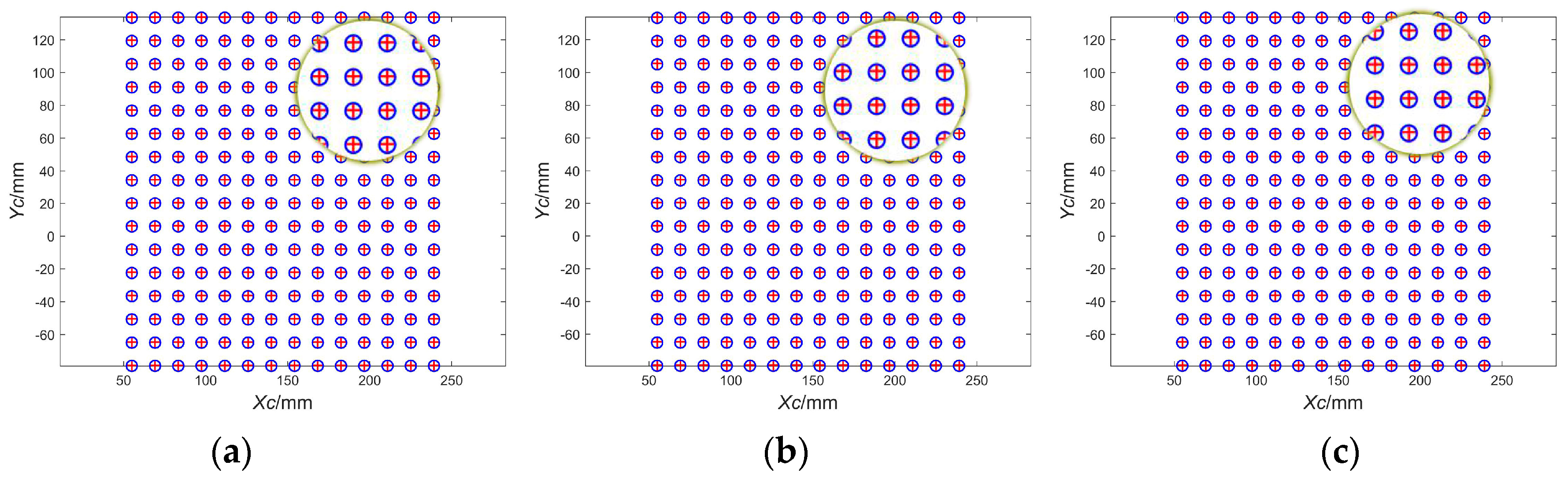
4.3.2. Camera Coordinates Registration of the Same Spatial Points Before and After Camera Rotation

In the experiment, we compared the camera coordinates of the spatial points on the target before and after camera rotation. Employing the imaging model, as shown in Figure 1b, the coordinates of spatial point P are (X_cl, Y_cl, Z_cl) and (X_cr, Y_cr, Z_cr) in camera coordinate system O_c1-X_c1Y_c1Z_c1 and O_c2-X_c2Y_c2Z_c2, respectively. If the plane O_c-X_cZ_c is parallel to plane O_w-Y_wZ_w, when the optical center coincides with the rotation center, the relationship between (X_cl, Y_cl, Z_cl) and (X_cr, Y_cr, Z_cr) is expressed by Equation (13),

$$\left[\begin{array}{c}{X}_{cl}\\ Y_{cl}\\ Z_{cl}\end{array}\right]=R_{\mathsf{\theta }}\left[\begin{array}{c}{X}_{cr}\\ Y_{cr}\\ Z_{cr}\end{array}\right],$$

(13)

where $R_{\mathsf{\theta }}=\left[\begin{array}{ccc}\cos \theta & 0& -\sin \theta \\ 0& 1& 0\\ \sin \theta & 0& \cos \theta \end{array}\right]$, and θ is the rotation angle of the turntable.

Otherwise, if the optical center deviates from the rotation center, the relationship between (X_cl, Y_cl, Z_cl) and (X_cr, Y_cr, Z_cr) should be expressed by Equation (14),

$$\left[\begin{array}{c}{X}_{cl}\\ Y_{cl}\\ Z_{cl}\end{array}\right]=R_{\mathsf{\theta }}\left[\begin{array}{c}{X}_{cr}\\ Y_{cr}\\ Z_{cr}\end{array}\right]+T,$$

(14)

where T is the translation vector between O_c1-X_c1Y_c1Z_c1 and O_c2-X_c2Y_c2Z_c2.

We shot the checkerboard images when the camera is rotated by the turntable with a different rotation angle θ_i and extracted checkerboard corners as marked points. Employing their homogeneous coordinates (X_wi, Y_wi, Z_wi, 1)^T in the world coordinate system, image coordinates (u_i, v_i, 1)^T, and the internal parameter matrix A, the rotation matrix R_i and translation vector T_i between the world coordinate system and the camera coordinate system at different position can be obtained from Equation (1). Then the coordinates (X_ci, Y_ci, Z_ci, 1)^T of the marked points can be calculated by Equation (15),

$$\left[\begin{array}{c}{X}_{ci}\\ Y_{ci}\\ Z_{ci}\\ 1\end{array}\right]=\left[\begin{array}{cc}{\mathit{R}}_i& {\mathit{T}}_i\\ 0^{\mathrm{T}}& 1\end{array}\right]\left[\begin{array}{c}{X}_w{}_i\\ Y_w{}_i\\ Z_{wi}\\ 1\end{array}\right].$$

(15)

Assume that (X_cl, Y_cl, Z_cl) and (X_cr, Y_cr, Z_cr) stand for the original coordinates and the coordinates after camera rotation of a spatial point, respectively. The coordinates (X’_cl, Y’_cl, Z’_cl) stands for the resulted coordinates calculated by Equation (13) from the coordinates (X_cr, Y_cr, Z_cr). We can compare (X’_cl, Y’_cl, Z’_cl) with the original coordinates (X_cl, Y_cl, Z_cl). If they are equal, it is proved that the optical center coincides with the rotation center; otherwise, it is indicated that the optical center of the camera deviates from the center of the turntable.

We first align the optical center with the rotation center by our proposed method. The camera captures the target images when the turntable rotates 0°, 6°, 9° and 12°, respectively, as shown in Figure 16. The original position of the camera corresponds to 0°. The coordinates (X_cl, Y_cl, Z_cl) and (X_cri, Y_cri, Z_cri) (i = 1, 2, 3) of the marked points are calculated, respectively. Employing Equation (13), (X’_cli, Y’_cli, Z’_cli) can be calculated by multiplying the corresponding rotation matrix R_θi. Comparing them with the coordinates (X_cl, Y_cl, Z_cl), we can see that the coordinates coincide accurately, as shown in Figure 17, where the original coordinates (X_cl, Y_cl, Z_cl) are marked as red “+” and the resulted coordinates (X’_cli, Y’_cli, Z’_cli) are marked as blue “o”; the circular zones are the enlarged parts. The standard deviation in the X_c and Y_c directions are shown in

Table 6. The standard deviation in the X_c and Y_c directions.

	Direction	STD/mm 6°	STD/mm 9°	STD/mm 12°
Alignment	Xc	0.010	0.048	0.065
	Yc	0.015	0.037	0.063
Misalignment	Xc	7.221	10.910	14.641
	Yc	0.314	0.358	0.424

.

We deviated the optical center from the rotation center and repeated the above steps. The captured target images are shown in Figure 18. When R_θi acts on the coordinates (X_cri, Y_cri, Z_cri) (i = 1, 2, 3) of the marked points, there is a significant deviation, as shown in Figure 19. The standard deviation in the X_c and Y_c directions are shown in Table 6.

The experiments verify that our method can align the optical center with the rotation center. When the optical center coincides with the rotation center, the extracted marked points coincide with each other when R_θi acts on the coordinates after camera rotation, and the alignment errors in the X_c and Y_c directions are quite small. Otherwise, the deviation in the X_c, Y_c direction is large.

5. Conclusions

We propose a method based on camera calibration with a two-dimensional target to solve the problem of the alignment of the camera’s optical center and the rotation center in a rotating optical measurement system composed of a camera and a rotating platform. An auxiliary plane coordinate system is introduced to adjust the external parameter matrix of the camera. The rectified external parameter matrix is used to calculate the optical centers in the unified world coordinate system. Multiple fitted circles can determine the rotation center more accurately than a single fitted circle, which will provide a higher precision in the following application, such as a panoramic mosaic. Simulations and experiments verified the effectiveness of the proposed method.

It should be noted that the optical center of the initial position of the camera should be kept at an appropriate distance from the rotation center during calibration to increase the accuracy of the circle fitting. By the way, although this paper only discusses the alignment of the optical center of the camera with a one-dimensional rotating optical system, the proposed method can also be extended in principle to the problem in the alignment of the optical center with the rotating axis of a two-dimensional rotating optical system. However, the current experimental setup is only suitable for the alignment problem of one-dimensional rotating optical systems. In the following work, we will find a device suitable for two-dimensional (pitch and yaw) rotating platforms.

References

1. Luhmann, T.; Robson, S.; Kyle, S.; Boehm, J. Close-Range Photogrammetry and 3D Imaging. Photogramm. Eng. Remote Sens. 2015, 81, 273–274. [Google Scholar]
2. Sun, T.; Xing, F.; You, Z. Optical system error analysis and calibration method of high-accuracy star trackers. Sensors (Basel) 2013, 13, 4598–4623. [Google Scholar] [CrossRef] [PubMed] [Green Version]
3. Luhmann, T. Close range photogrammetry for industrial applications. ISPRS J. Photogramm. Remote Sens. 2010, 65, 558–569. [Google Scholar] [CrossRef]
4. Robert, S.; Holger, B.; Armin, K.; Richard, K. Measurement of three-dimensional deformation vectors with digital holography and stereo photogrammetry. Opt. Lett. 2012, 37, 1943–1945. [Google Scholar]
5. Li, J.; Liu, Z. Efficient camera self-calibration method for remote sensing photogrammetry. Opt. Express 2018, 26, 14213–14231. [Google Scholar] [CrossRef] [Green Version]
6. Zhang, S. Three-dimensional range data compression using computer graphics rendering pipeline. Appl. Opt. 2012, 51, 4058–4064. [Google Scholar] [CrossRef] [Green Version]
7. Li, Y.; Wang, H.; Ma, L.; Shi, Y. Three-dimensional imaging and display of real-existing scene using fringe. In Proceedings of the Volume 8769, International Conference on Optics in Precision Engineering and Nanotechnology (icOPEN2013), Singapore, 22 June 2013; Quan, C., Qian, K., Asundi, A., Eds.; p. 87691I1-9. [Google Scholar]
8. Sun, P.; Lu, N.; Dong, M. Modelling and calibration of depth-dependent distortion for large depth visual measurement cameras. Opt. Express 2017, 25, 9834–9847. [Google Scholar] [CrossRef]
9. Xiao, Y.; Su, X.; Chen, W.; Liu, Y. Three-dimensional shape measurement of aspheric mirrors with fringe reflection photogrammetry. Appl. Opt. 2012, 51, 457–464. [Google Scholar] [CrossRef]
10. Huang, S.; Zhang, Z.; Ke, T.; Tang, M.; Xu, X. Scanning Photogrammetry for Measuring Large Targets in Close Range. Remote Sens. 2015, 7, 10042–10077. [Google Scholar] [CrossRef] [Green Version]
11. Tomasi, C.; Zhang, J. How to rotate a camera. In Proceedings of the 10th International Conference on Image Analysis and Processing, Venice, Italy, 27–29 September 1999; pp. 606–611. [Google Scholar]
12. Gledhill, D.; Tian, G.; Taylor, D.; Clarke, D. Panoramic imaging—A review. Comput. Graph. 2003, 27, 435–445. [Google Scholar] [CrossRef]
13. Luhmann, T. A historical review on panorama photogrammetry. Int. Arch. Photogramm. Remote Sens. Spat. Inf. Sci. 2004, 34, 8. [Google Scholar]
14. Kukko, A. A new method for perspective centre alignment for spherical panoramic imaging. Photogramm. J. Finl. 2004, 19, 37–46. [Google Scholar]
15. Kauhanen, H.; Rönnholm, P.; Lehtola, V.V. Motorized panoramic camera mount-calibration and image capture. ISPRS Ann. Photogramm. Remote Sens. Spat. Inf. Sci. 2016, 3, 89–96. [Google Scholar] [CrossRef]
16. Huang, Y. 3-D measuring systems based on theodolite-CCD cameras. Int. Arch. Photogramm. Remote Sens. Spat. Inf. Sci. 1993, 29, 541. [Google Scholar]
17. Huang, Y. Calibration of the Wild P32 camera using the camera-on-theodolite method. Photogrammetric Rec. 1998, 16, 97–104. [Google Scholar] [CrossRef]
18. Andreas, W. A new approach for geo-monitoring using modern total stations and RGB + D images. Measurement 2016, 82, 64–74. [Google Scholar]
19. Zhang, Z.; Zheng, S.; Zhan, Z. Digital terrestrial photogrammetry with photo total station. Int. Arch. Photogramm. Remote Sens. Istanb. Turk. 2004, 232–236. [Google Scholar]
20. Zhang, Z.; Zhan, Z.; Zheng, S. Photo total station systemthe integration of digital photogrammetry and total station. Bull. Surv. Mapp. 2005, 11, 1–5. [Google Scholar]
21. Zhang, X.; Zhu, Z.; Yuan, Y.; Li, L.; Sun, X.; Yu, Q.; Ou, J. A universal and flexible theodolite-camera system for making accurate measurements over large volumes. Opt. Lasers Eng. 2012, 50, 1611–1620. [Google Scholar] [CrossRef]
22. Huang, L.; Zhang, Q.; Asundi, A. Flexible camera calibration using not-measured imperfect target. Appl. Opt. 2013, 52, 6278–6286. [Google Scholar] [CrossRef]
23. Huang, L.; Zhang, Q.; Asundi, A. Camera calibration with active phase target: Improvement on feature detection and optimization. Opt. Lett. 2013, 38, 1446–1448. [Google Scholar] [CrossRef] [PubMed]
24. Wang, Y.; Wang, Y.; Liu, L.; Chen, X. Defocused camera calibration with a conventional periodic target based on Fourier transform. Opt. Lett. 2019, 44, 3254–3257. [Google Scholar] [CrossRef] [PubMed]
25. Fischler, M.A.; Bolles, R.C. Random sample consensus: A paradigm for model fitting with applications to image analysis and automated cartography. Commun. ACM 1981, 24, 381–395. [Google Scholar] [CrossRef]
26. Gao, X.; Hou, X.; Tang, J.; Cheng, H. Complete solution classification for the perspective-three-point problem. IEEE Trans. Pattern Anal. Mach. Intell. 2003, 25, 930–943. [Google Scholar]
27. Zhang, Z. A flexible new technique for camera calibration. IEEE Trans. Pattern Anal. Mach. Intell 2000, 22, 1330–1334. [Google Scholar] [CrossRef] [Green Version]
28. Gander, W.; Golub, G.H.; Strebel, R. Least-squares fitting of circles and ellipses. BIT 1994, 34, 558–578. [Google Scholar] [CrossRef]
Figure 1. (a) Schematic diagram of the rotating optical measurement system; (b) schematic diagram of the imaging model.
Applsci 10 06962 g001
Figure 2. Schematic diagram of the coordinate systems.
Applsci 10 06962 g002
Figure 3. The flow chart of the procedure.
Applsci 10 06962 g003
Figure 4. The rotation diagram of the camera placed at positions c1, c2 and c3.
Applsci 10 06962 g004
Figure 5. The rotation diagram of the simulated camera placed at positions Cr, Cg and Cb.
Applsci 10 06962 g005
Figure 6. (a) Projection of the simulated optical centers on the YwOwZw plane without noise; (b) projection of the simulated optical centers on the YwOwZw plane with 3.5% Gaussian noise.
Applsci 10 06962 g006
Figure 7. (a) Fitted circular curve without noise; (b) fitted circular curve with 3.5% Gaussian noise.
Applsci 10 06962 g007
Figure 8. (a) Experimental setup; (b) one set of the patterns for calibration.
Applsci 10 06962 g008
Figure 9. (a) Graph of the rotation angles γix(j), γiy(j) and γiz(j); (b) graph of the rectified rotation angles γix(j), γiy(j) and γiz(j).
Applsci 10 06962 g009
Figure 10. (a) Projection of the optical centers on the YwOwZw plane; (b) fitted circular curve (red*, green* and blue* are the fitted centers of the three fitted curves marked by c1, c2 and c3, respectively).
Applsci 10 06962 g010
Figure 11. (a) Projection of the optical centers on the YwOwZw plane; (b) fitted circular curve.
Applsci 10 06962 g011
Figure 12. Photocentric coordinate distribution map.
Applsci 10 06962 g012
Figure 13. Schematic diagram.
Applsci 10 06962 g013
Figure 14. Marker points.
Applsci 10 06962 g014
Figure 15. (a) The angle curves when coaxial; (b) the difference curves of the adjacent angles when coaxial; (c) the angle curves when off-axis; (d) the difference curves of the adjacent angles when off-axis.
Applsci 10 06962 g015
Figure 16. The checkerboard images of (a) 0°; (b) 6°; (c) 9°; (d) 12°.
Applsci 10 06962 g016
Figure 17. The comparative diagrams of the marked points of (a) 6°; (b) 9°; (c) 12°.
Applsci 10 06962 g017
Figure 18. The checkerboard images of (a) 0°; (b) 6°; (c) 9°; (d) 12°.
Applsci 10 06962 g018
Figure 19. The comparative diagrams of the marked points of (a) 6°; (b) 9°; (c) 12°.
Applsci 10 06962 g019