Static and Dynamic Responses of Micro-Structured Beams


Abstract
1. Introduction
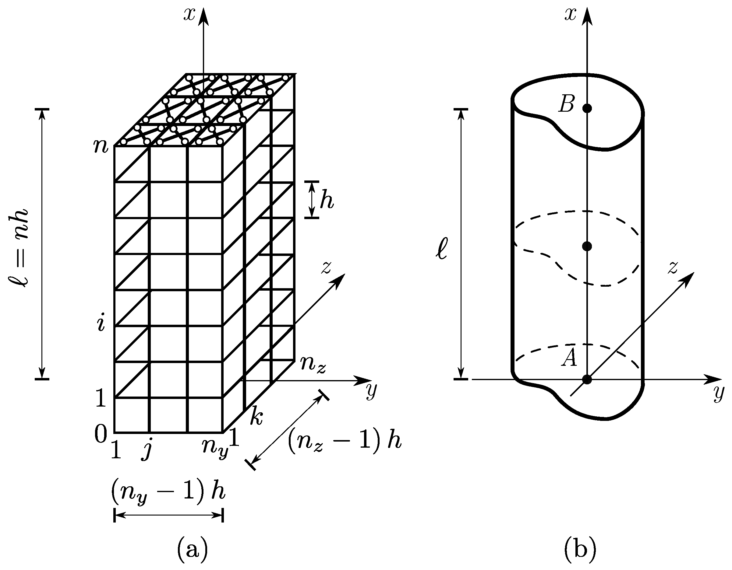
2. Model
- Clamped at A and free at B: ;
- Simply-supported and torsionally restrained in A, B: .
- Clamped at A and free at B: ;
- Simply supported and torsionally restrained in A, B: .
- Clamped at A and free at B:
- Simply-supported and torsionally restrained in A, B:
3. Elastic and Inertial Constant Identifications
3.1. Identification Algorithm for the Elastic Constants
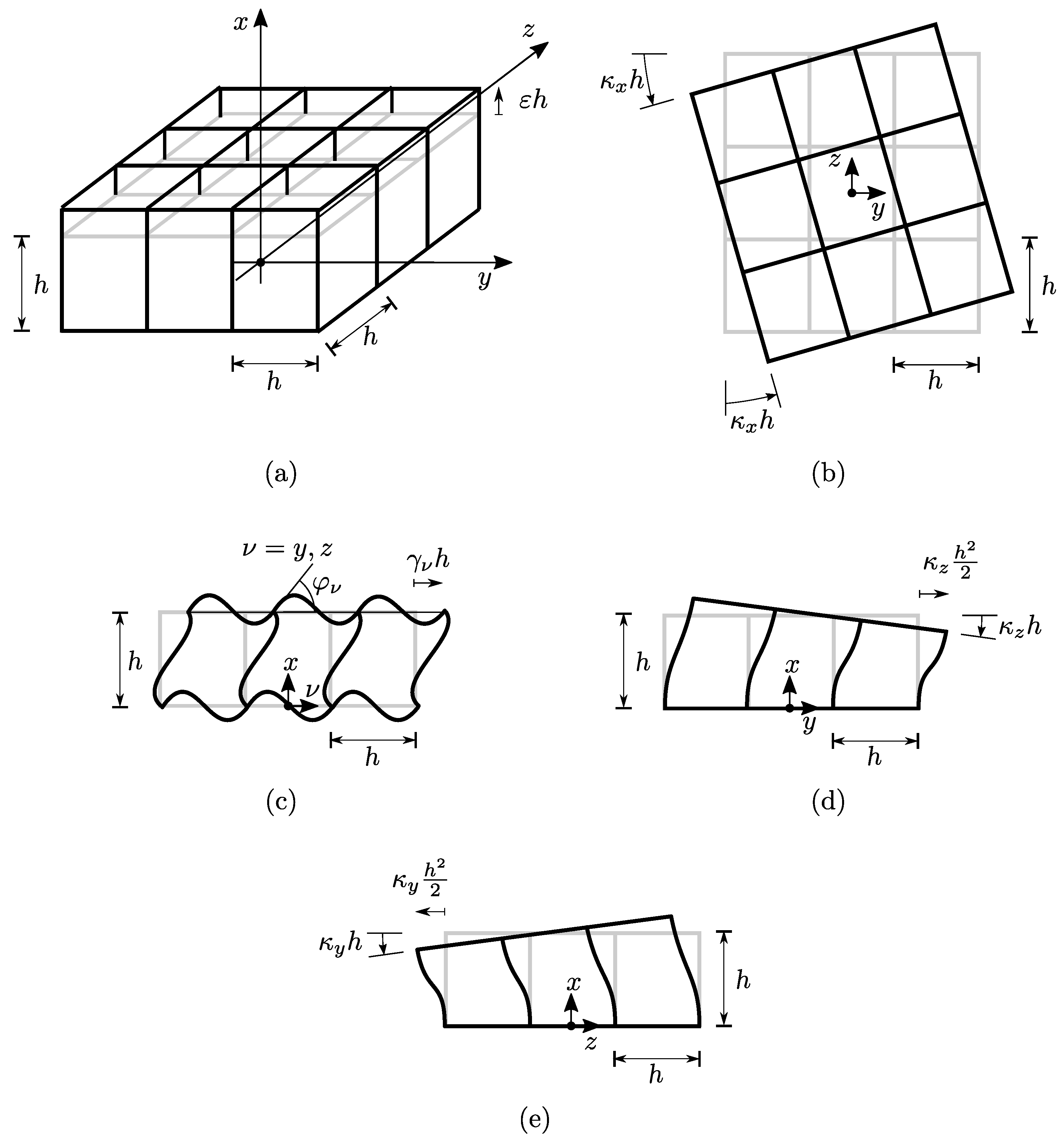
- An extensional mode (), in which translates axially;
- Two shear modes (, ), in which translates transversely along the y- and z-directions, respectively;
- two flexural modes (, ), in which rotates around the y- and z- axes, respectively, and translates transversely along the z- and y- axes;
- A torsional mode (), in which rotates around the x- axis.
Analytical Identification of Elastic Constants of the Grid Beam
- That due to their bending in the cross-section plane;
- That due to their torsion.
3.2. Identification of the Inertial Properties
4. Numerical Results
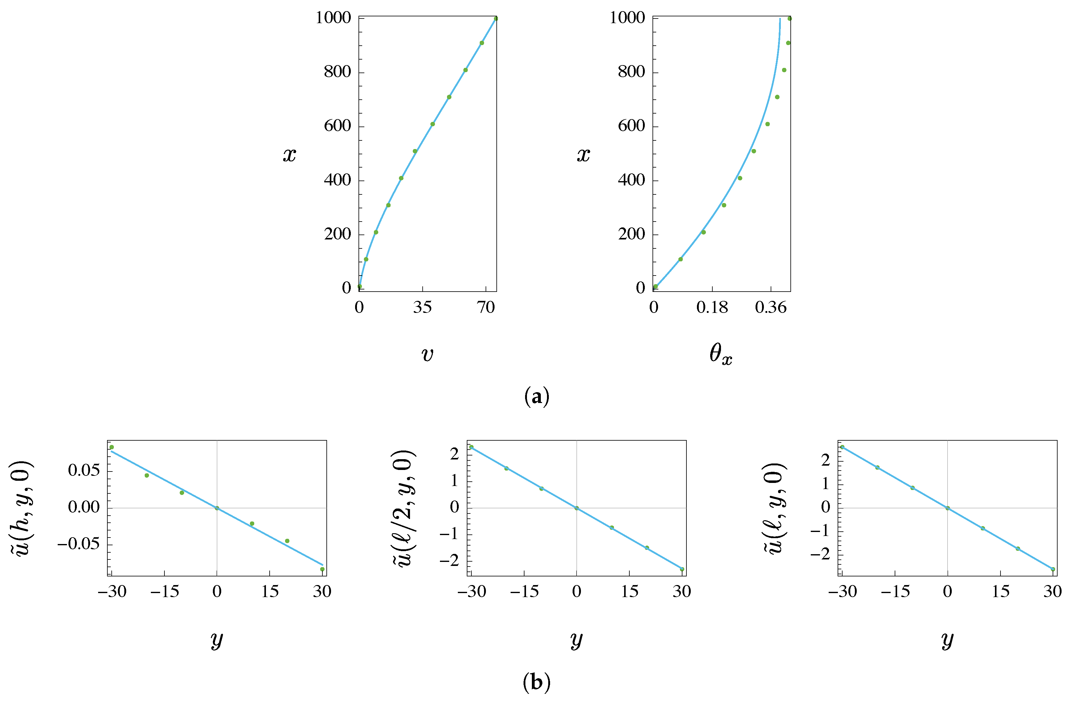
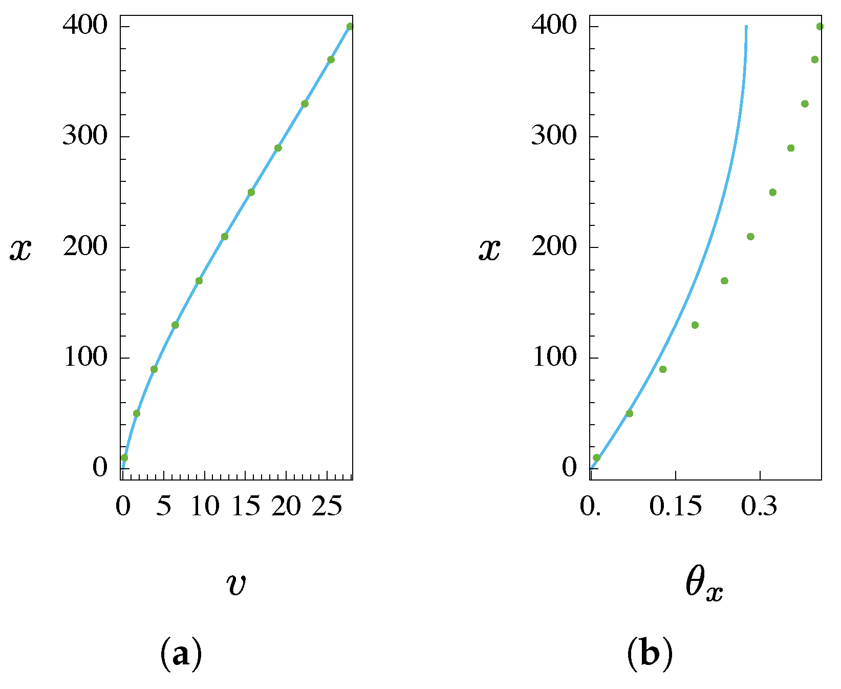
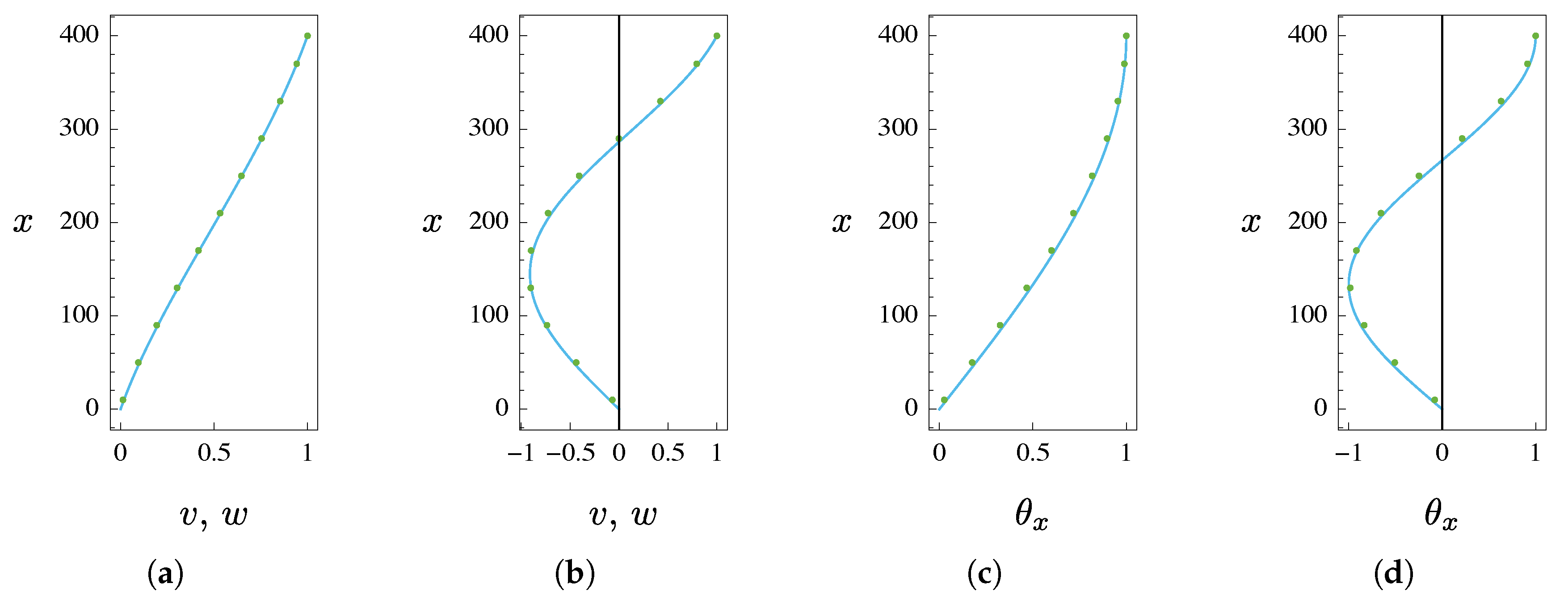
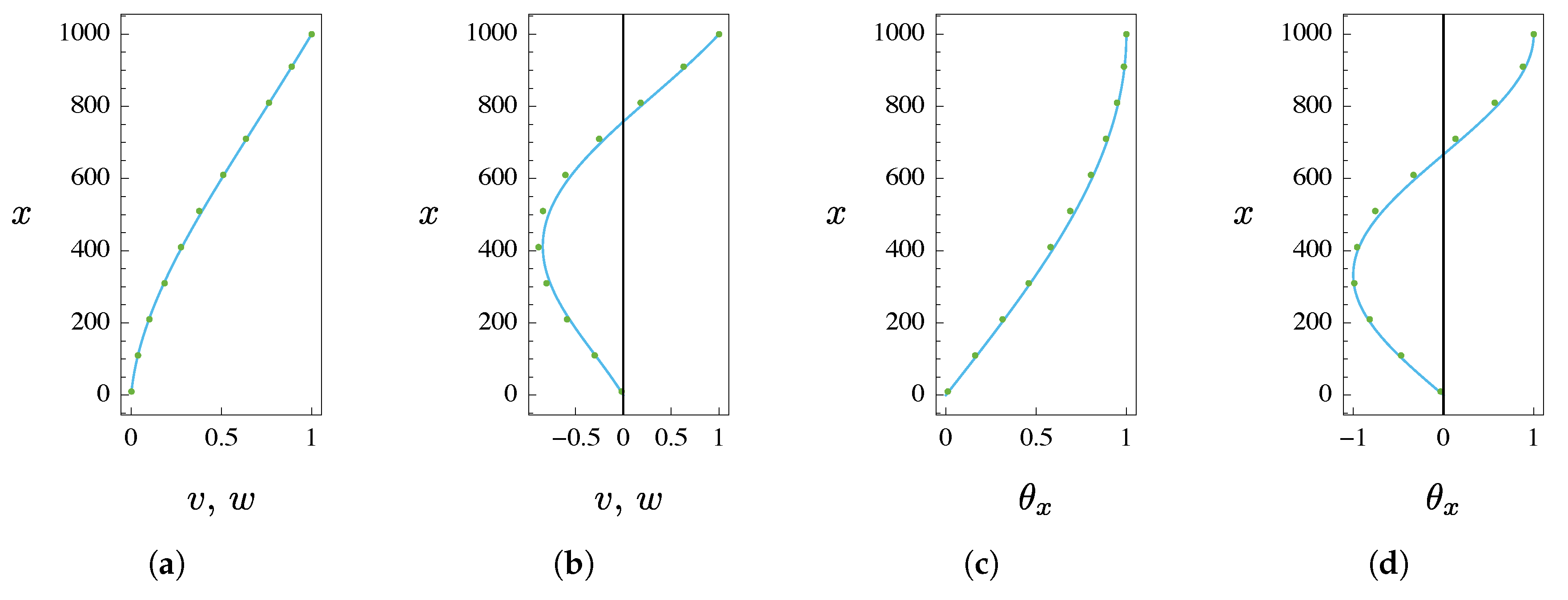
4.1. Statics
- case I: (TO mode) and (au-TO mode);
- case II: (TO mode) and (au-TO mode).
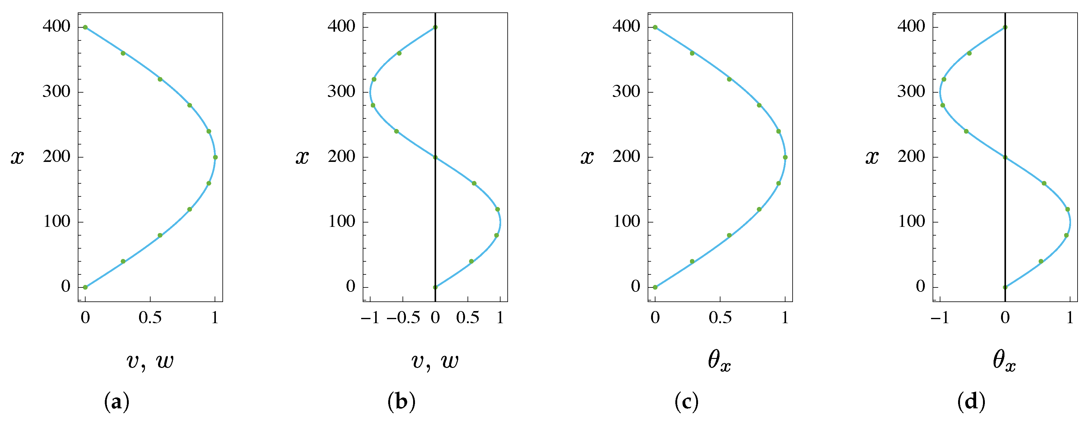
4.2. Dynamics
5. Conclusions and Perspectives
- An excellent accuracy in terms of translational displacements is given by the Timoshenko model, both in statics and in free dynamics (modal shapes), independently from the number of cells.
- An excellent agreement between coarse and fine models is also detected, both in statics and in free dynamics (modal shapes), for torsional displacements, where when the aspect ratio of the grid beam cross-section is close to 1, this circumstance reduces the effect of macro-warping. In contrast, when the cross-section is thin, significant errors due to macro-warping appear.
- Very good agreement is also detected in terms of natural frequencies. In this case, the macro-warping effect also entails worsening of the accuracy in the torsional modes.
Author Contributions
Funding
Conflicts of Interest
References
- Maconachie, T.; Leary, M.; Lozanovski, B.; Zhang, X.; Qian, M.; Faruque, O.; Brandt, M. SLM lattice structures: Properties, performance, applications and challenges. Mater. Des. 2019, 183, 108137. [Google Scholar] [CrossRef]
- Mieszala, M.; Hasegawa, M.; Guillonneau, G.; Bauer, J.; Raghavan, R.; Frantz, C.; Kraft, O.; Mischler, S.; Michler, J.; Philippe, L. Micromechanics of amorphous metal/polymer hybrid structures with 3D cellular architectures: Size effects, buckling behavior, and energy absorption capability. Small 2017, 13, 1602514. [Google Scholar] [CrossRef] [PubMed]
- Casalotti, A.; D’Annibale, F.; Rosi, G. Multi-scale design of an architected composite structure with optimized graded properties. Compos. Struct. 2020, 252, 112608. [Google Scholar] [CrossRef]
- Askar, A.; Cakmak, A.S. A structural model of a micropolar continuum. Int. J. Eng. Sci. 1968, 6, 583–589. [Google Scholar] [CrossRef]
- Dos Reis, F.; Ganghoffer, J.F. Construction of micropolar continua from the asymptotic homogenization of beam lattices. Comput. Struct. 2012, 112, 354–363. [Google Scholar] [CrossRef]
- Noor, A.K. Continuum modeling for repetitive lattice structures. Appl. Mech. Rev. 1988, 41, 285–296. [Google Scholar] [CrossRef]
- Tollenaere, H.; Caillerie, D. Continuous modeling of lattice structures by homogenization. Adv. Eng. Softw. 1998, 29, 699–705. [Google Scholar] [CrossRef]
- Di Nino, S.; Luongo, A. A simple homogenized orthotropic model for in-plane analysis of regular masonry walls. Int. J. Solids Struct. 2019, 167, 156–169. [Google Scholar] [CrossRef]
- Hache, F.; Challamel, N.; Elishakoff, I.; Wang, C. Comparison of nonlocal continualization schemes for lattice beams and plates. Arch. Appl. Mech. 2017, 87, 1105–1138. [Google Scholar] [CrossRef]
- Boutin, C.; Hans, S.; Chesnais, C. Generalized Beams and Continua. Dynamics of Reticulated Structures. In Mechanics of Generalized Continua: One Hundred Years After the Cosserats; Maugin, G.A., Metrikine, A.V., Eds.; Springer: New York, NY, USA, 2010; pp. 131–141. [Google Scholar]
- Boutin, C.; dell’Isola, F.; Giorgio, I.; Placidi, L. Linear pantographic sheets: Asymptotic micro-macro models identification. Math. Mech. Complex Syst. 2017, 5, 127–162. [Google Scholar] [CrossRef]
- dell’Isola, F.; Eremeyev, V.A.; Porubov, A. Advances in Mechanics of Microstructured Media and Structures; Springer: Cham, Switzerland, 2018; Volume 87. [Google Scholar]
- dell’Isola, F.; Seppecher, P.; Spagnuolo, M.; Barchiesi, E.; Hild, F.; Lekszycki, T.; Giorgio, I.; Placidi, L.; Andreaus, U.; Cuomo, M.; et al. Advances in pantographic structures: Design, manufacturing, models, experiments and image analyses. Contin. Mech. Thermodyn. 2019, 31, 1231–1282. [Google Scholar] [CrossRef]
- dell’Isola, F.; Seppecher, P.; Alibert, J.J.; Lekszycki, T.; Grygoruk, R.; Pawlikowski, M.; Steigmann, D.; Giorgio, I.; Andreaus, U.; Turco, E.; et al. Pantographic metamaterials: An example of mathematically driven design and of its technological challenges. Contin. Mech. Thermodyn. 2019, 31, 851–884. [Google Scholar] [CrossRef]
- Giorgio, I.; Rizzi, N.L.; Turco, E. Continuum modelling of pantographic sheets for out-of-plane bifurcation and vibrational analysis. Proc. R. Soc. A Math. Phys. Eng. Sci. 2017, 473, 20170636. [Google Scholar] [CrossRef]
- De Angelo, M.; Barchiesi, E.; Giorgio, I.; Abali, B.E. Numerical identification of constitutive parameters in reduced-order bi-dimensional models for pantographic structures: Application to out-of-plane buckling. Arch. Appl. Mech. 2019, 89, 1333–1358. [Google Scholar] [CrossRef]
- Challamel, N.; Hache, F.; Elishakoff, I.; Wang, C. Buckling and vibrations of microstructured rectangular plates considering phenomenological and lattice-based nonlocal continuum models. Compos. Struct. 2016, 149, 145–156. [Google Scholar] [CrossRef]
- Hache, F.; Challamel, N.; Elishakoff, I. Lattice and continualized models for the buckling study of nonlocal rectangular thick plates including shear effects. Int. J. Mech. Sci. 2018, 145, 221–230. [Google Scholar] [CrossRef]
- Chajes, M.J.; Romstad, K.M.; McCallen, D.B. Analysis of multiple-bay frames using continuum model. J. Struct. Eng. 1993, 119, 522–546. [Google Scholar] [CrossRef]
- Zalka, K.A. Global Structural Analysis of Buildings; CRC Press: Boca Raton, FL, USA, 2002. [Google Scholar]
- Potzta, G.; Kollár, L. Analysis of building structures by replacement sandwich beams. Int. J. Solids Struct. 2003, 40, 535–553. [Google Scholar] [CrossRef]
- Boutin, C.; Hans, S. Homogenisation of periodic discrete medium: Application to dynamics of framed structures. Comput. Geotech. 2003, 30, 303–320. [Google Scholar] [CrossRef]
- Hans, S.; Boutin, C. Dynamics of discrete framed structures: A unified homogenized description. J. Mech. Mater. Struct. 2008, 3, 1709–1739. [Google Scholar] [CrossRef]
- Chesnais, C.; Boutin, C.; Hans, S. Structural Dynamics and Generalized Continua. In Mechanics of Generalized Continua; Altenbach, H., Maugin, G., Erofeev, V., Eds.; Springer: Berlin/Heidelberg, Germany, 2011; pp. 57–76. [Google Scholar]
- Luongo, A. Statics, Dynamics, Buckling and Aeroelastic Stability of Planar Cellular Beams. In Modern Trends in Structural and Solid Mechanics; Challamel, N., Kaplunov, J., Takewaki, I., Eds.; ISTE-Wiley: Hoboken, NJ, USA, 2020. [Google Scholar]
- Piccardo, G.; Tubino, F.; Luongo, A. A shear–shear torsional beam model for nonlinear aeroelastic analysis of tower buildings. Z. Für Angew. Math. Und Phys. 2015, 66, 1895–1913. [Google Scholar] [CrossRef]
- Piccardo, G.; Tubino, F.; Luongo, A. Equivalent nonlinear beam model for the 3-D analysis of shear-type buildings: Application to aeroelastic instability. Int. J. Non-Linear Mech. 2016, 80, 52–65. [Google Scholar] [CrossRef]
- Piccardo, G.; Tubino, F.; Luongo, A. Equivalent Timoshenko linear beam model for the static and dynamic analysis of tower buildings. Appl. Math. Model. 2019, 71, 77–95. [Google Scholar] [CrossRef]
- Ferretti, M. Flexural torsional buckling of uniformly compressed beam-like structures. Contin. Mech. Thermodyn. 2018, 30, 977–993. [Google Scholar] [CrossRef]
- D’Annibale, F.; Ferretti, M.; Luongo, A. Shear-shear-torsional homogenous beam models for nonlinear periodic beam-like structures. Eng. Struct. 2019, 184, 115–133. [Google Scholar] [CrossRef]
- Di Nino, S.; Luongo, A. Nonlinear aeroelastic behavior of a base-isolated beam under steady wind flow. Int. J. Non-Linear Mech. 2020, 119, 103340. [Google Scholar] [CrossRef]
- Ferretti, M.; D’Annibale, F.; Luongo, A. Buckling of tower-buildings on elastic foundation under compressive tip-forces and self-weight. Contin. Mech. Thermodyn. 2020. [Google Scholar] [CrossRef]
- Luongo, A.; Zulli, D. Free and forced linear dynamics of a homogeneous model for beam-like structures. Meccanica 2020, 55, 907–925. [Google Scholar] [CrossRef]
- Luongo, A.; D’Annibale, F.; Ferretti, M. Shear and flexural factors for homogenized beam models of planar frames. Eng. Struct. 2020, submitted. [Google Scholar]
- Ferretti, M.; D’Annibale, F.; Luongo, A. Modeling beam-like planar structures by a one-dimensional continuum: An analytical-numerical method. J. Appl. Comput. Mech. 2020, in press. [Google Scholar]
- Eugster, S.; Steigmann, D. Continuum theory for mechanical metamaterials with a cubic lattice substructure. Math. Mech. Complex Syst. 2019, 7, 75–98. [Google Scholar] [CrossRef]
- Antman, S.S. The theory of rods. In Linear Theories of Elasticity and Thermoelasticity; Springer: Berlin/Heidelberg, Germany, 1973; pp. 641–703. [Google Scholar]
- Antman, S.S. Nonlinear Problems of Elasticity; Springer: New York, NY, USA, 2005. [Google Scholar]
- Capriz, G. A Contribution to the Theory of Rods. Riv. Mat. Univ. Parma 1981, 7, 489–506. [Google Scholar]
- Luongo, A.; Zulli, D. Mathematical Models of Beams and Cables; John Wiley & Sons: Hoboken, NJ, USA, 2013. [Google Scholar]
- Altenbach, H.; Bîrsan, M.; Eremeyev, V.A. Cosserat-type rods. In Generalized Continua from the Theory to Engineering Applications; Springer: Wien, Austria, 2013; pp. 179–248. [Google Scholar]
- Steigmann, D.J.; Faulkner, M.G. Variational theory for spatial rods. J. Elast. 1993, 33, 1–26. [Google Scholar] [CrossRef]
- Elishakoff, I. Handbook on Timoshenko-Ehrenfest Beam and Uflyand-Mindlin Plate Theories; World Scientific: Singapore, 2020. [Google Scholar]
- Cazzani, A.; Stochino, F.; Turco, E. On the whole spectrum of Timoshenko beams. Part I: A theoretical revisitation. Z. Für Angew. Math. Und Phys. 2016, 67, 24. [Google Scholar] [CrossRef]
- Cazzani, A.; Stochino, F.; Turco, E. On the whole spectrum of Timoshenko beams. Part II: Further applications. Z. Für Angew. Math. Und Phys. 2016, 67, 25. [Google Scholar] [CrossRef]
- Silvestre, N.; Camotim, D. First-order generalised beam theory for arbitrary orthotropic materials. Thin-Walled Struct. 2002, 40, 755–789. [Google Scholar] [CrossRef]
- Ranzi, G.; Luongo, A. A new approach for thin-walled member analysis in the framework of GBT. Thin-Walled Struct. 2011, 49, 1404–1414. [Google Scholar] [CrossRef]
- Taig, G.; Ranzi, G.; D’Annibale, F. An unconstrained dynamic approach for the generalised beam theory. Contin. Mech. Thermodyn. 2015, 27, 879–904. [Google Scholar] [CrossRef]


| 4905 | 2043.75 | 919.69 | 778.06 |
| Case Study I | Case Study II | ||
|---|---|---|---|
| m | |||
| Case Study | Mode | Description (F = Flexural, T = Torsional) | |||
|---|---|---|---|---|---|
| I-a, | 1, 2 | 1st F -plane, 1st F -plane | 195.58 | 188.92 | 3.5 |
| 3 | 1st T | 280.76 | 271.05 | 3.6 | |
| 4, 5 | 2nd F -plane, 2nd F -plane | 641.16 | 624.07 | 2.7 | |
| 6 | 2nd T | 842.27 | 816.63 | 3.1 | |
| I-a, | 1, 2 | 1st F -plane, 1st F -plane | 42.82 | 42.16 | 1.6 |
| 3 | 1st T | 112.30 | 107.81 | 4.2 | |
| 4, 5 | 2nd F -plane, 2nd F -plane | 192.60 | 187.28 | 2.8 | |
| 6 | 2nd T | 336.91 | 324.03 | 4.0 | |
| I-b, | 1, 2 | 1st F -plane, 1st F -plane | 437.76 | 433.86 | 0.9 |
| 3 | 1st T | 561.51 | 557.96 | 0.6 | |
| 4, 5 | 2nd F -plane, 2nd F -plane | 988.03 | 979.15 | 0.9 | |
| 6 | 2nd T | 1123.03 | 1119.60 | 0.3 | |
| II-a, | 1 | 1st F -plane | 116.03 | 113.80 | 2.0 |
| 2 | 1st F -plane | 211.03 | 203.81 | 3.5 | |
| 3 | 1st T | 287.47 | 238.38 | 20.1 | |
| 4 | 2nd F -plane | 503.20 | 496.07 | 1.4 | |
| 5 | 2nd F -plane | 693.98 | 673.15 | 3.1 | |
| 6 | 2nd T | 862.42 | 743.75 | 16.0 |
© 2020 by the authors. Licensee MDPI, Basel, Switzerland. This article is an open access article distributed under the terms and conditions of the Creative Commons Attribution (CC BY) license (http://creativecommons.org/licenses/by/4.0/).
Share and Cite
D’Annibale, F.; Ferretti, M.; Luongo, A. Static and Dynamic Responses of Micro-Structured Beams. Appl. Sci. 2020, 10, 6836. https://doi.org/10.3390/app10196836
D’Annibale F, Ferretti M, Luongo A. Static and Dynamic Responses of Micro-Structured Beams. Applied Sciences. 2020; 10(19):6836. https://doi.org/10.3390/app10196836
Chicago/Turabian StyleD’Annibale, Francesco, Manuel Ferretti, and Angelo Luongo. 2020. "Static and Dynamic Responses of Micro-Structured Beams" Applied Sciences 10, no. 19: 6836. https://doi.org/10.3390/app10196836
APA StyleD’Annibale, F., Ferretti, M., & Luongo, A. (2020). Static and Dynamic Responses of Micro-Structured Beams. Applied Sciences, 10(19), 6836. https://doi.org/10.3390/app10196836