Evaluation of Long-Range Mobile Mapping System (MMS) and Close-Range Photogrammetry for Deformation Monitoring. A Case Study of Cortes de Pallás in Valencia (Spain)

Abstract

This contribution describes the methodology applied to evaluate the suitability of a Long-Range Mobile Mapping System to be integrated with other techniques that are currently used in a large and complex landslide deformation monitoring project carried out in Cortes de Pallás, in Valencia (Spain). Periodical geodetic surveys provide a reference frame realized by 10 pillars and 15 additional check points placed in specific points of interest, all with millimetric accuracy. The combined use of Close-Range Photogrammetry provides a well-controlled 3D model with 1–3 cm accuracy, making the area ideal for testing new technologies. Since some zones of interest are usually obstructed by construction, trees, or lamp posts, a possible solution might be the supplementary use of dynamic scanning instruments with the mobile mapping solution Kaarta Stencil 2 to collect the missing data. However, the reliability of this technology has to be assessed and validated before being integrated into the existing 3D models in the well-controlled area of Cortes de Pallás. The results of the experiment show that the accuracy achieved are compatible with those obtained from Close-Range Photogrammetry and can also be safely used to supplement image-based information for monitoring with 3–8 cm overall accuracy.

1. Introduction

The evaluation of deformations in civil infrastructures or natural environments is normally assessed by the realization of very accurate three-dimensional (3D) models by means of a range of complementary geomatics techniques such as total stations, global navigation satellite systems (GNSS), photogrammetry, or laser scanning [1]. Nonetheless, each geomatic technique is affected by its own instrumental and physical limitations, especially when the monitored area is large and has a complex topography [2]. For instance, atmospheric refraction can severely limit the achievable accuracy in the distance and angular measurements, also in laser and image scanning [3]. Therefore, the integration of data, collected by different techniques, in a unique coordinate reference frame becomes crucial to producing consistent 3D models able to be used for overtime deformation monitoring purposes [4].

In recent decades, advanced monitoring technologies have spread and increasingly been used for the study and management of geological hazard and risk, which may compromise the state of preservation of civil infrastructure [5]. Monitoring actions are necessary to guarantee health and safety conditions by controlling the evolution of deformation patterns or detecting significant instabilities. In terms of spatial and temporal resolution, the improvement of geomatics techniques represents a significant achievement. These methods provide innovative tools in supporting mapping products and geological analysis required for assessment and evaluation. Accurate and fully geo-referenced 3D datasets can be used to characterize in detail structural and geological settings, as well as the geomorphology of a studied area. Geological applications, for example, geo-hydrological risk assessment, rockfall runout modellings, or slope stability analysis, can have a great benefit through non-destructive investigation.

Where a topographic survey is based on limited distances (e.g., tens to hundreds of meters), it has historically been carried out with total stations. Although such method provides high accuracy and precision for the measurement of individual points, significant time is required to collect a sufficient density of data to produce rough landscape Digital Elevation Models (DEMs) [6]. Laser Scanning (LS) and Close-Range Photogrammetry (CRP) are state of the art techniques for acquiring dense and precise topographic data at the output detail, for accurate volume measurements or modeling.

Accurate mapping and monitoring of lakeside reservoirs, as well as coastal areas and fluvial processes, are critical tasks to which several techniques have been used, from aerial photographs, remote sensing, land surveying, CRP and, more recently Terrestrial Laser Scanning (TLS) and Mobile Laser Scanning (MLS). These latter technologies are in principle advantageous because of their good accuracy, easiness of use and lower time of response [7].

Most of the existing geomatics techniques are sometimes unaffordable, and there is not an all-in-one solution able to provide spatial information with suitable accuracy and temporal frequency. For the completion of existing surveys in particular, MLS was considered the most suitable alternative for the challenges established in the project requirements, concerning productivity, sample density and final costs. In particular, Mobile Mapping System (MMS) technology enables users to reach complex and enclosed spaces, either scanning by hand or by attaching a scanner to a trolley, drone, or mounting on a pole. As a result, the variety of difficult-to-survey environments becomes wider. This solves the problem linked to GNNS-based systems where it does not work well in complex contexts, for example, woods, where tree canopies block signals, as occurred in this case study. With no reliance on remote data, MMS are a priori a truly go-anywhere technology.

In this paper, a comparison of a long-range handheld MMS with the CRP has been evaluated that offers particular promise for site-scale topographic surveys. Experiments were conducted exploiting the case study of Cortes de Pallas [2], where three-year period monitoring surveys have been undertaken with sub-millimetric electronic distance meter (EDM) techniques and CRP. The result of the survey consists of a 3D model where the combination of these techniques ensures a complete mapping of the site, avoiding the creation of gaps in the point clouds thanks to the compensation of one technique on the other and vice versa. This 3D model provides a basis for the analysis of the rocky landslide deformation monitoring. The main contribution of this manuscript is to demonstrate how MMS can complement the 3D mapping of a challenging environment, by integrating multi-source data in a unique reference frame and with an accuracy comparable with other state of art methods. Several tests are presented, providing the research community with guidelines that will be useful for other similar settings, presenting the MMS as an alternative approach when other geomatic methods fail.

This article is structured as follows: after a first state-of-the-art review in using MLS for mapping and monitoring purposes, Section 3 describes the geomatics techniques used for the data acquisition in the selected case study. Section 4 focuses on the data processing and the integration of georeferenced point clouds from MMS with the CRP. In Section 5 the results of this comparison are evaluated to assess the accuracy achieved in the combination of these data. The discussion and conclusion are finally presented in Section 6 and Section 7.

2. Related Work

Mobile mapping systems are becoming popular as they can build 3D point clouds of any type of environment rapidly by using a laser scanner that is integrated with a navigation system. The laser scanner is able to record millions of points. The files with the point clouds can be viewed, navigated, measured and analyzed as discrete 3D models. The evolution of the laser scanner as a surveying technique has resulted in this tool being used not only to obtain an optimal geometric reconstruction of the scene, but also to assess changes in a particular state.

Mobile LiDAR (Light Detection And Ranging) technology presents some advantages: high-speed data capture through reduction of time and cost, remote acquisition and measurement increasing survey in efficiency and safety, high point density data ensuring a comprehensive representation of the detected scene, an abundance of data acquired in movement. The light weight of these MLSs makes them flexible and versatile instruments, so they can be mounted on any mobile platform. In places with complex topography, the use of MMS, following a continuous path, is more advantageous than a tripod-based laser scanner that requires multiple scan positions to cover all the areas of the survey [6]. Moreover, integrating MMS with other geomatics techniques, such as Digital Photogrammetry (DP), allows giving an added value and greater richness of the acquired data providing a high detailed DEM or DTM (Digital Terrain Model) of the selected area [8].

Alternative purposes to use mobile LiDAR technologies, in addition to the assessment of the geometrical state, concern change detection, deformation analysis [9], hazard assessment and structural and infrastructural health monitoring [4] in different types of natural environment. In technical terms, mobile mapping solutions contemporaneously allow users to acquire geometrical aspects for geological studies and geomorphological analysis, to operate mapping of all the elements present in the detected area (e.g., vegetation, road, etc.), and to define basic modeling for monitoring operations (e.g., rockfalls, coastal erosion, river dynamics, etc.). Examples described by literature are various, depending on natural effects as geological and atmospheric actions or anthropogenic consequences of the built environment which compromise the stability of the natural landscape.

The major case studies that include the use of MLS for mapping and monitoring purposes are those related to geomorphology detection and landscape dynamics such as landslides and rockfall displacements. The combination of MLS and DP can greatly improve the realization of detailed modeling of the geometrical discontinuity of a slope to analyze a landslide susceptibility and potential rockfall mechanisms [9]. Examples of slope stability assessment through the kinematic method are applied in rock outcrops in British Columbia, Canada, and Carrara marble quarry, Italy [10]. The use of MLS was presented by Francioni et al. [11] in a geological study of landslides applied to an interesting case study in Normandy. They used a boat-based MMS to scan 3D point clouds of unstable coastal cliffs to detect rockfalls and erosional deposits. A similar case is proposed by [12] who described a new approach of coastal cliff monitoring, in Poland, which is based on a combination of MLS from the sea with the geotechnical stability calculations. A 3D mapping was carried out by an airborne MMS, installed on a helicopter, to monitor a small landslide in the North Yorkshire coast in the UK. As a result, more accurate modeling of the terrain was obtained, especially areas covered by vegetation [13]. A ground-based approach was evaluated by James et al. [5] using a handheld MLS to collect topographic data in complex terrain as a gully site at the coastal cliff in Sunderland, UK. To carry out the survey, the hand-held mobile device is walked around the site following a close loop path to facilitate accurate 3D reconstruction and avoiding problems associated with drift.

Landslides happen also inside residential areas causing cracks to buildings and drainage, for example, the study area located in a Malaysian city. Here, to monitor an active landslide, researchers used MLS to assess the movements of the land, in both vehicle-based and human-based mode in a complementary way to acquire completely the surface of the study area [14].

Mobile mapping solutions have been also applied in change detection and deformation analysis for sandy dunes and river courses. The adoption of MLS was illustrated by Nahon et al. [15] that provides an accurate and robust method to obtain high resolution space-time datasets along a Dutch beach useful to understand the changes of dunes volume, under the influence of both marine and aeolian processes. The MLS was carried out mounting the device on a car and using airborne LiDAR to process several DEMs of the sandy dunes. The monitoring of beach dunes is needed to improve the scientific observation of their dynamics. A test was realized in Cap Ferret, France, where researchers combined MLS with aerial photogrammetry to deliver accurate 3D reconstruction of the dunes. They confirmed the good results of using mobile mapping devices for their high level of detail and greater spatial coverage [16]. The best results were also achieved in monitoring the lagoon area of Padre Island National Seashore, located in Texas, where mobile scanning devices may be preferred for the detailed and comprehensive final DEMs useful to detect 3D terrain features and so to monitor geomorphic changes [17].

These challenging trials prove that a mobile LiDAR system, in recent years, has emerged as a viable alternative for surveying coastal beaches and foredunes, but also for riverine topography. Measurements were conducted by Vaaja et al. [18] using an MMS mounted on a boat and mounted on a manually-operated cart to define the riverine topography and modeling in 3D of the coarse fluvial sediment along the river Tenojoki, in Finland. The application of a MMS was tested by Williams et al. [19] for a complex relief and the following reconstruction of fluvial surface sedimentology and topography of river Feshie, in Scotland.

Monitoring actions also occur to control the actual state of civil infrastructures, for example, the maintenance of pavement condition of roads to detect instabilities and to assure safe conditions. It is possible to detect the road surface on 3D models derived from a dense point cloud acquired by MLS. LiDAR instruments are suitable to collect data with adequate accuracy and high resolution for mapping and inventory purposes, and, also, the surveyors can make surveys safely with minimal interruptions of the traffic flow [9]. The use of accurate and dense point cloud data along a route corridor enables the detection of surface distortion, joints, cracks and other roughness conditions [20]. Also retaining walls along roads needs to be monitored to assess their stability, especially in mountainous regions to support either roads or slopes adjacent to roads. An efficient method was proposed by Lienhart et al. [21] based on a mobile mapping system to detect a retaining wall used to construct a highway, in Austria. The MMS, mounted on a car, generated a high-density point cloud where tilt changes of the structure can be calculated to define the current state of the structure itself. The 3D model helped to recognize forms of damage and their distribution on the surface of the wall, thus compensating for the typical punctual analysis carried out with the total station. Moreover, referring to the case study presented in that article, among the monitored infrastructures they also include water reservoirs and hydroelectric power plants. A boat-based MMS was selected by Brazilian researchers to scan the progression of marginal erosion in different reservoirs of hydroelectric plants. The processed point clouds and rendered meshes and the creation of cross-sections were used to compute the rate and the dynamics of the erosion phenomenon [6,22].

3. Data Acquisition

Since 2017, a monitoring plan to the rock-wall of the lakeside reservoir has been commissioned by the Infrastructures Area of the Diputació de València. This change detection operation is performed yearly. After a first geodetic survey to detect fixed targets and select some check points, the data acquisition was carried out with a reflex camera for a CRP from different points of view to cover the whole area of interest. In 2019, in addition to the two techniques mentioned, a third survey was added: the MMS was tested to make this type of survey more complete, and verified through a comparison operation between point clouds. The combination of the two surveys had the objective of completing the 3D mapping of the site, needed to support the monitoring plan of the rock-wall.

3.1. Cortes de Pallás Test Site

Cortes de Pallás is a Cretaceous limestone area with historical geotechnical issues. On 6 April 2015, a cliff called La Muela partially collapsed, and some facilities of the electricity power plant and the main access road to the village were seriously damaged. At the end of 2017, once the consolidation works were finished, the Infrastructures Area of the Diputació de València commissioned a deformation monitoring plan to detect possible displacements of huge boulders or potential malfunction of the installed anchoring systems [2]. However, the detection of possible displacements of some centimeters with the required level of significance in a short period, e.g., two or three years, is a quite challenging task that can only be approached by means of high-precision geodetic techniques due to the peculiar topography of the zone. The whole area involves distances from 500 to 2000 m with height differences reaching 500 m. Moreover, 10 geodetic pillars mounted on presumably stable locations at 15 target points (referred to as check points) were installed in the rock wall by professional climbers using abseiling techniques, because they are not directly accessible. Furthermore, the measurements have to be undertaken by necessity from the opposite shoreline which is about 600 m away because the cliff of interest is facing a water reservoir (Figure 1).

Therefore, the Diputació de València opted for periodical geodetic surveys along with image-based techniques like CRP and long-range TLS (since 3D models derived from CRP and TLS techniques proved compatible, only the former will be use for the experiment) as the most feasible join solution for the deformation monitoring plan. The periodical geodetic surveys, which are based on sub-millimetric EDM techniques and performed annually, have a triple objective: (i) to establish and monitor a high-precision 3D reference frame realized by 10 pillars, coded 8000+ (Figure 2a), (ii) to determine the 3D coordinates of 15 additional check points, represented by 360° prisms coded 1000+ (Figure 2b and Figure 3) placed in specific points of interest on the monitored rock wall, and (iii) to provide a ground control network for image-based techniques.

As a demonstration of the potentiality of the high-precision geodetic techniques used [23,24], the displacements found for the reference frame pillars between the years 2018 and 2019 are shown in

Table 1. Displacement of the reference frame pillars obtained by using sub-millimetric electronic distance meter (EDM) techniques between years 2018 and 2019. Points with statistical T above the cut-off value 5.739 are considered to have a significative displacement with a 99% probability. Pillar 8006 was not measured in the 2018 campaign.

Pillar	Displacements and Their Corresponding Errors			Deformation
No.	Dx (mm)	Dy (mm)	Dz (mm)	T	Conclusion
8001	1.23 ± 0.70	0.84 ± 0.48	−2.45 ± 1.74	1.253	No
8002	0.42 ± 0.37	0.32 ± 0.34	3.31 ± 1.80	3.340	No
8003	0.87 ± 0.27	0.72 ± 0.37	0.48 ± 1.23	3.457	No
8004	0.28 ± 0.70	−1.11 ± 0.52	−3.51 ± 3.37	1.952	No
8005	0.58 ± 0.61	−1.48 ± 0.67	−6.12 ± 2.29	11.609	Yes
8007	−0.43 ± 0.65	−1.35 ± 0.97	−0.80 ± 1.95	1.272	No
8008	0.15 ± 0.59	0.57 ± 0.50	1.87 ± 1.75	1.024	No
8009	0.21 ± 0.47	2.11 ± 0.66	−5.55 ± 2.59	4.858	No
8010	−0.00 ± 0.99	−1.51 ± 0.58	1.10 ± 1.49	3.477	No

. Except for pillar number 8005 (Figure 2a), where a significative vertical displacement of −6.12 mm (see Table 1) was detected, the reference frame can be considered stable and well-controlled. The resulting reference frame has an overall accuracy of 1 mm and its scale is metrologically consistent with the unit of length of the International System (SI). Further information about the geodetic surveys is given in Section 3.2.

This high-precision geodetic method, which is very demanding and time-consuming, can be only applied to a limited number of relevant points of interest, which are 15 targets in the case at hand. Complementary geomatic techniques like long-range TLS or CRP are needed to massively collect information with a density of around 300 points/m². However, the accuracy of this type of points is reduced up to 1 to 3 cm. The main problem with both geomatic techniques is that photographs and cloud points provided by respectively CRP and TLS need to be registered in the same reference frame. In the case at hand, the reference frame as well as the coordinates of the 15 check points of interest, which are periodically provided by the sub-millimetric geodetic techniques, are considered the ground truth for the integration of the three techniques so that the combined numeric models are fully consistent.

An additional problem with both CRP and TLS techniques, especially when they are performed statically, like in the case at Cortes de Pallás, is the presence of occlusions. Since the CRP images can easily miss some shadowed areas, the 3D model obtained in each campaign usually has small patches with no information. A possible and efficient solution could be the use of mobile mapping solutions like the Kaarta Stencil 2 (https://www.kaarta.com/products/stencil-2-for-rapid-long-range-mobile-mapping/). Being dynamic, this system can provide a continuous 3D survey of the problematic area in Cortes de Pallás in less than one hour.

However, prior to being accepted as part of the combined 3D numeric models, the consistency of the points cloud obtained with the Kaarta system has to prove that it is consistent with the data provided by the EDM and CRP techniques. Since EDM and CRP are compatible at the 1–3 cm level (see

Table 2. Differences between the close-range photogrammetry (CRP) and the EDM coordinates obtained for the check points.

Target	Differences CRP—EDM (mm)
	Δx	Δy	Δz	Total
1001	13.1	23.9	21.9	35.0
1002	9.7	21.2	8.3	24.7
1003	4.9	18.7	16.2	25.2
1004	−0.6	6.5	12.3	13.9
1005	5.0	11.3	1.5	12.5
1006	3.2	−9.4	7.9	12.7
1007	−11.8	−11.8	2.1	16.8
1008	11.3	23.0	−3.9	25.9
1009	12.9	13.7	3.8	19.2
1010	9.8	−7.7	10.5	16.3
1011	16.8	−13.2	12.5	24.7
1012	0.5	−19.0	19.9	27.5
1013	3.5	−17.8	−0.1	18.1
1014	12.4	−10.5	3.3	16.6
1015	13.7	14.9	9.4	22.3

), the point cloud obtained with the Kaarta system can be compared with the CRP solution in two ways to facilitate the analysis: first, using the dense CRP point cloud; second, employing manually measured natural photogrammetric check points.

3.2. Geodetic Survey

The reference frame is a geodetic network with 10 concrete pillars that surround the 15 check points. Pillars and target points (Figure 2) were set up in 2017. Each target point consists of one Leica 360 reflector (RFL) and one standard target sphere (Ø145 mm) which are rigidly mounted and firmly attached to the rock.

Since their installation had to be undertaken by abseiling, their verticality cannot be taken for granted. The determination of their attitude, which is crucial to transfer coordinates between the center for distances and the center for images, was obtained by photogrammetric methods. Figure 3 shows the photogrammetric data acquisition followed to obtain the vector and thus their attitude between centers.

So far, two geodetic campaigns have been carried out by using a sub-millimetric EDM Kern ME5000 Mekometer (ME5000) [25,26]. For each distance measurement, the meteorological parameters were measured and double-checked by using a traditional Thies Clima Assmann-Type psychrometer (±0.2 K) and a Thommen 3B4.01.1 aneroid barometer (±0.3 hPa) along with a network of 10 Testo 176P1 data-loggers. All the meteorological sensors were previously calibrated at the Universitat Politècnica de Valencia (UPV) calibration laboratory.

Prior to the EDM adjustment, the following corrections were applied: refraction correction [27,28,29], EDM frequency drift correction and geometric correction [25]. Once these corrections were applied and their corresponding errors computed in order to contribute to the stochastic model, the resulting slope distances were 3D adjusted in the local coordinate system CP2017 (x,y,z) in two steps. In the first step, only distances between pillars were adjusted to provide a solution for the frame. In the second step, distances to check points are included in order to obtain their 3D coordinates. The applied method not only provides coordinates with an overall accuracy of 0.5–1 mm for pillars and 1–3 mm for check points, respectively, but also allows us to monitor the possible displacement of pillars (see Table 1). Finally, the EDM coordinates and their precisions were also converted into geodetic coordinates with ellipsoidal height (φ,λ,h) and TM30 with orthometric height (E,N,H) [2].

As it can be seen in Table 2, the differences between the CRP and the EDM coordinates that were obtained in November 2019 are in the range of 1 to 3 cm, which are the expected values and demonstrates that the sub-millimetric EDM-based coordinates are consistent with the CRP-based 3D numeric model that is used as ground truth to validate the accuracy of the CRP survey.

3.3. Close-Range Photogrammetry

The geometry of the site is rather peculiar, with a huge reservoir in front of the hillside (Figure 1), with many crossing hydroelectric power lines from one side to the other, which hamper the exploitation of close-range imagery with RPAS–UAVs (remotely piloted aircraft system–unmanned aerial vehicles). The approximate dimension of the interest hillside displayed in Figure 1 (yellow box) is 700 m wide and 200 m high. In addition, pictures were taken not from ideally planned positions but realistically ideal positions on-site, after defining some minimum constraints such as ideal ground sampling distance (GSD) e.g., following roads parallel to the hillside, and from surrounding hills.

For the CRP campaign, two 21 Mpix full-frame cameras were used mounted on stable tripods: Canon EOS D5 Mark II with a normal Canon EF 50 mm f/1.4 USM lens, and a Canon 1Ds Mark III with a telephoto Canon EF 200 mm f/2,8 L II USMlens (Figure 4). The first camera was used to get the whole area, summing 280 normal and convergent imagery; the second camera was used to measure only three areas with the fixed on-the-rock 15 check points, summing 404 imagery. The data acquisition was planned to achieve a GSD of 3.5 cm. The mean camera-object distance was 512 m. A total of 6 h were devoted to taking images on site.

The three-step workflow followed to achieve accuracy better than 3 cm is presented next. First step, each camera was calibrated on the job selecting a subsampled ideal network with convergent and rotated imagery, summing up to 57 images for the 50 mm lens and 47 images for the 200 mm lens. For the normal lens, 8 interior orientation parameters (f, cx, cy, K1, K2, K3, P1, P2) were computed to achieve 0.34 pixel image reprojection error; for the telephoto lens, 4 additional parameters (f, cx, cy, K1) were computed to achieve a 0.50 pixel image reprojection error. Second step, a free bundle block adjustment with 230 imagery (142 normal + 88 tele) was undertaken. This step included the manual measurement of the white spherical targets (Figure 2b and Figure 3) on the imagery, including 4 (visible) control points on pillars of the reference frame and 15 check points (Figure 5). A mean reprojection error of 0.50 pixels was achieved in the photogrammetric adjustment. Third step, absolute orientation by means of a 3D similarity transformation yielding an RMSE (root mean square error) of 1.55 cm.

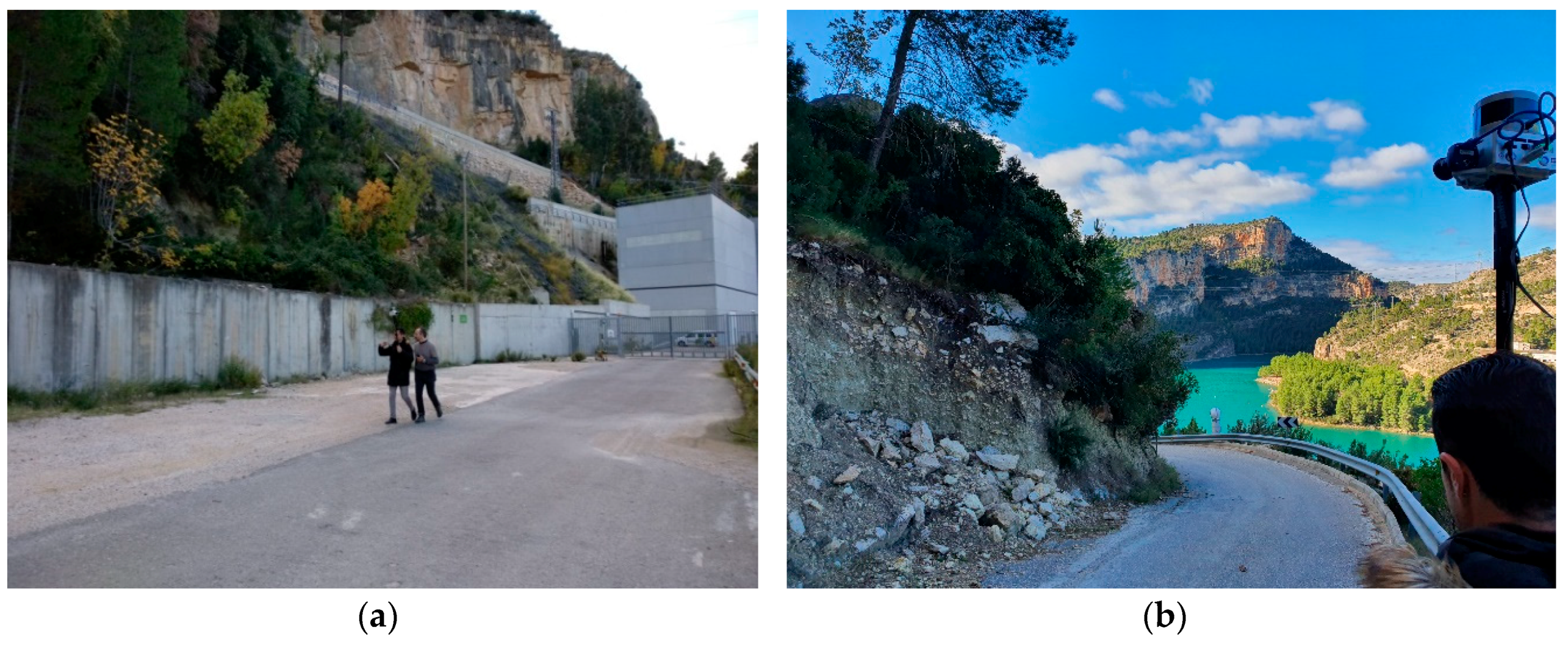
3.4. Mobile Mapping System

After the acquisition phases performed by EDM and CRP campaigns, a survey with the MMS was conducted. As previously stated, despite the high accuracy reached with the aforementioned methods, visual occlusions and vegetation prevented the whole mapping; mainly the streets and the lower parts of the rock walls could not be surveyed. Kaarta Stencil 2 is a stand-alone, lightweight instrument, with an integrated system of mapping and real-time position estimation. An MMS consists mainly of three components: mapping sensors for data acquisition, a positioning and navigation unit for data localization and a time referencing unit for data recording [30]. Kaarta Stencil 2 depends on LiDAR consisting of a Velodyne VLP-16, connected to a low-cost MEMS (micro electro-mechanical system) IMU (inertial measurement unit) and a processing computer for localization and real-time mapping. VLP-16 has a maximum laser range of 100 m and 360° horizontal FOV (field of view) with a 30° azimuthal opening with a band of 16 laser beams. The LiDAR has a centimetric accuracy with a value variation of ±30 mm and a speed of 300,000 points per second. The acquisition phase was carried out using the appropriate configuration parameters, set for outdoor environments, that include values for the voxelSize, namely the resolution of the point cloud in the map file, for cornerVoxelSize, surfVoxelSize, sorroundVoxelSize, those indicate the resolution of the point cloud for scan matching and display, and for blindRadius, that is the minimum distance of the points to be used for the mapping (

Table 3. Parameters setting of Kaarta Stencil 2, optimized for outdoor scenario.

Parameters	Default Value [m]
voxelSize	0.4
cornerVoxelSize	0.2
surfVoxelSize	0.4
surroundVoxelSize	0.6
blindRadius	2.0

).

In realizing this ground-based survey characterized by a long path on foot, walking along the edge of the road, the laser scanner was mounted on a small pole held by hand (Figure 6). Human-based LS has not been widely used in the monitoring of rock slopes, but in this case study was useful to detect areas of the surveyed region not clearly visible through the CRP. The MMS needed to fill the gaps of the photogrammetric 3D model, such as roads or parts obstructed by the crown of trees, that the photogrammetric camera cannot reach from the different points of view to detect all the features.

The data acquisition operation was performed following a closed path (close-loop) [31,32], to facilitate accurate reconstruction of the surveyed region and avoid problems associated with drift, where the beginning and end of the route coincide [3]. In Cortes de Pallás test site the surveyor completed a trajectory (backwards and forwards) of 2.9 km long in total, at an average distance of 3–5 m from the rock wall, acquired in 1 h and 43 min, collecting over 480 billion points (

Table 4. Scan info of the estimated trajectory executed with mobile mapping system (MMS) Kaarta Stencil 2.

Scan Information
Filename	/2019-11-27-10-58-50/scan_info_2019-11-27-10-58.yaml
Launch mode	Mapping with Camera
Time Stats
Start Time (y-m-d; h:m:s)	2019-11-27; 10:59:02
Stop Time (y-m-d; h:m:s)	2019-11-27; 12:42:27
Scan Time (h:m:s)	01:43:25
Point Cloud Stats
Average Confidence	218,943.715342
Number of Points	482,799,466
Trajectory Length	2905.259698 m
Trajectory Points	25,414
File Size	11,587,187,366 Byte

).

A tracker camera, integrated to the mobile mapping device, needs to show and save the trajectory made during the acquisition operations. The progress of the scanning can be monitored in real-time via an external monitor attached with a USB cable. At the end of the acquisition phase with Kaarta Stencil 2, information about the configuration setting, the 3D point cloud characteristics, the estimated trajectory is stored in a folder automatically created by the MMS processer at every operation of the survey.

4. Data Processing

4.1. Close-Range Photogrammetry (CRP) Point Cloud Processing

The next steps in the photogrammetric processing were devoted to yield as accurately as possible the 3D model of the hillside. 43.58 million points were obtained for the site area, reaching a mean density of 413 points/m². The mean distance among points in the 3D point cloud is 7.6 cm. All the steps presented up to this point were processed with Agisoft PhotoScan Professional v. 1.4.4 build 6848. However, for filtering the point cloud, 3DReshaper was used. Noisy points were removed with the option delete points (over 20 cm). Afterward, from the segmented point cloud, tiny sets of points (below 11) were automatically deleted. Next, extensive manual filtering was undertaken to remove points identified as vegetation (trees and shrubs) or isolated points outside of the ground such as power poles or road signs. The result of this phase is visible in Figure 7, which presents the difference in a sector without and after filtering. The final number of points was 42.75 million points.

4.2. Mobile Mapping System (MMS) Point Cloud Processing

The open-source software CloudCompare has been used to process the 3D point cloud by MMS, with the purpose of analysing the raw data acquired (Figure 8). As a default parameter, the number of points composing the sharpened MMS point cloud is 94.30 million.

In order to obtain ground and non-ground points from MLS point cloud, the data filtering algorithm Cloth Simulation Filter (CSF) was used [33]. This method allows users to obtain the “steep slope” model setting some advanced parameters such as cloth resolution, maximum iterations and classification threshold (

Table 5. Advanced parameters applied to cloth simulation filter (CSF) operation to perform the segmentation between ground and non-ground points.

Cloth Resolution	Maximum Iterations	Classification Threshold
0.5	n. 150	0.5

). The cloth resolution refers to the grid size of cloth composed by particles interconnected through virtual springs, which is used to cover the terrain. The positions of the particles in three-dimensional space determine the position and shape of the cloth. The grid size has the same unit of the point cloud. The lower the value of cloth resolution, the softer the resulting mesh from the filtered point cloud is. The number of iterations is linked to the maximum iteration times of terrain simulation. Classification threshold is used to classify ground and non-ground points, based on the distances between points and the simulated terrain.

The final output is a segmentation of the MMS cloud, where all the vertical features, like trees, pylons and road signs, were automatically removed (Figure 9), reducing the number of points to 47.86 million.

4.3. MMS Point Cloud Georeferencing

Since a GNSS system was not integrated with Kaarta Stencil 2, the georeferencing of the point cloud could be realized in two ways: using the control points captured by the EDM or aligning the point cloud to the CRP model, already georeferenced. As only EDM points fell within the path trajectory, the second option has been chosen and represents a completely new experiment tested by the Kaarta manufacturing experts. The filtered CRP point cloud presented in Figure 10 was thus used next as the control system for the MMS point cloud.

After the filtering operation of the MMS point cloud, the next step consisted of roughly aligning the trajectory of Kaarta Stencil 2 with the CRP point cloud. First, the yaw angle of the starting point of the MMS close-loop trajectory in the CRP point cloud was identified and calculated. Then, the parameters of the MMS point cloud could be set up iteratively to obtain a better result in the replay operation of the trajectory line, evaluating every time the correspondence with the photogrammetry point cloud. Defined as the right alignment of the trajectory, the MMS point cloud was run following this adjusted close-loop line and automatically adapted with the same roto-translation transformation. At the end of this procedure, the two point clouds were overlapped and so they could be analyzed by executing a comparison operation between the point clouds themselves (Figure 11).

5. Result Comparison

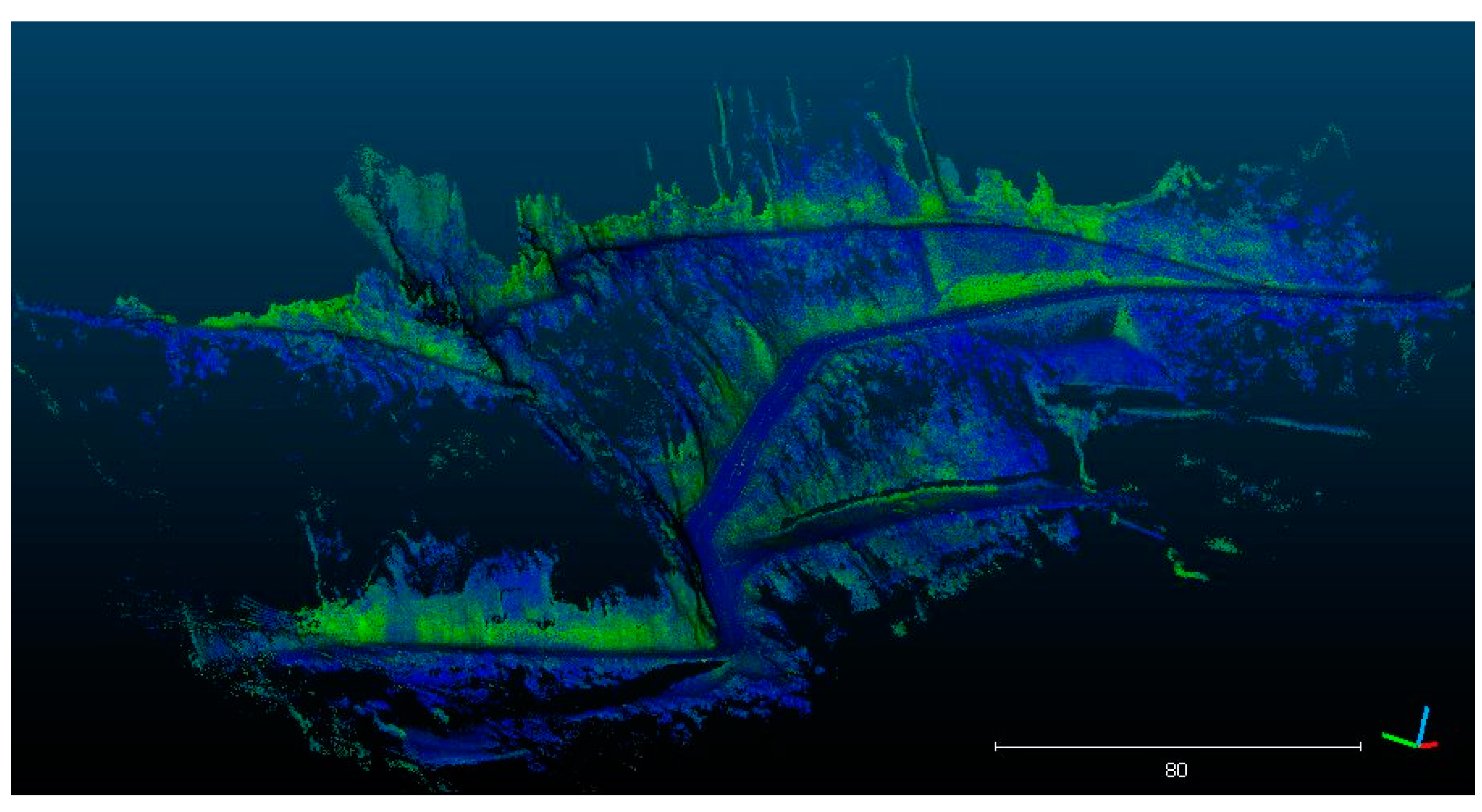
The resulting combination (Figure 12) of the point clouds from MMS and CRP surveys was assessed using the cloud-to-cloud (C2C) distance tool. The C2C tool exploits the nearest neighbour algorithm to compute the Euclidean distance between each point of the compared cloud and the nearest point of the reference cloud [32].

First, we computed the “closest point set” [34] applied to the CRP point cloud. This tool is useful for understanding which points of the CRP point cloud are closest to each point of the MMS cloud.

Taking the MMS point cloud as a reference, a new CRP point cloud was generated, preserving only the closest points. This new point cloud represents a new base for the C2C distance calculation.

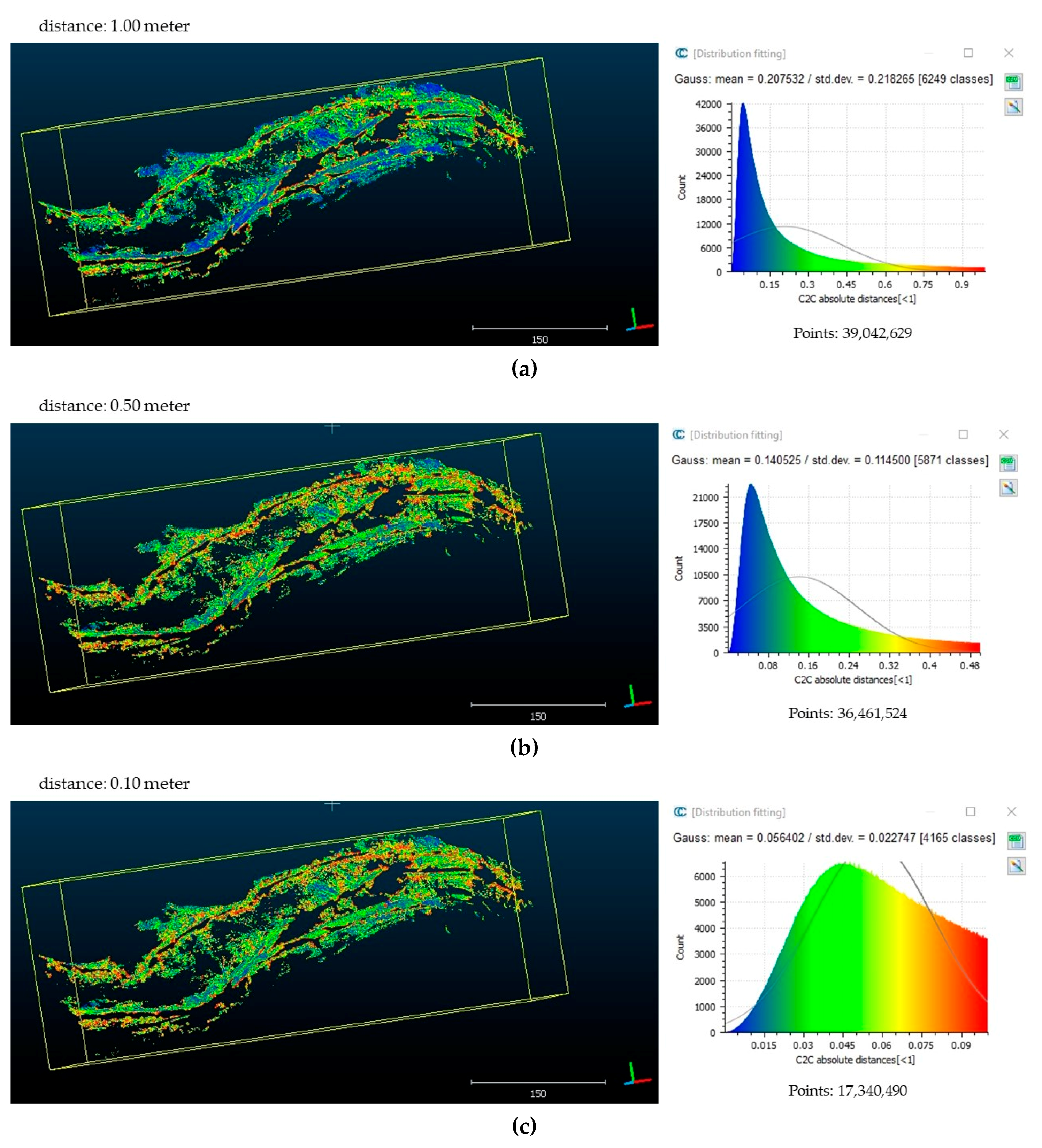
Then, the C2C distance was calculated by taking the resampled CRP point cloud as a reference and setting the point distances in different ranges, from 1.00 to 0.10 m to evaluate different computations in term of RMSE, standard deviation and number of points (Figure 13).

Analyzing Figure 13, it can be noted that setting the distance computation at 1 m between the two point clouds, we have lost almost 8.8 million points with respect to the original one. The former value represents the points that have any correspondence in the CRP point cloud, excluding then the parts of the roads that cannot be seen from the camera due to the occlusions. The threshold of 0.50 m between the two point clouds was computed to understand better the distribution fitting of C2C absolute distance. In the end, we set the C2C distance computation at 0.10 m. The choice of this threshold value is motivated by the fact that long-range MMS and CRP are techniques characterized by sub-decimeter accuracy. The number of points has become low: 17 million points of MMS have a higher correspondence with the CRP point cloud. From the results of the point clouds assessment, it emerges that, at 0.10 m distance, a mean difference of 5.6 cm between laser scanner and photogrammetry exits, with a standard deviation of 2.3 cm (Figure 13).

The reduction of the number of points during the different distance computations can be explained as follows: first, the MMS point cloud is denser than the CRP “closest point set” point cloud, so only a low number of points between the two point clouds has the nearest correspondence; second, the MMS point cloud is noisier. The decrease of the number of points in MMS point clouds during the phases of the C2C evaluation does not imply an information waste, since the remaining 30 million points of MMS point clouds are partially useful to fill the “holes” of the CRP point cloud.

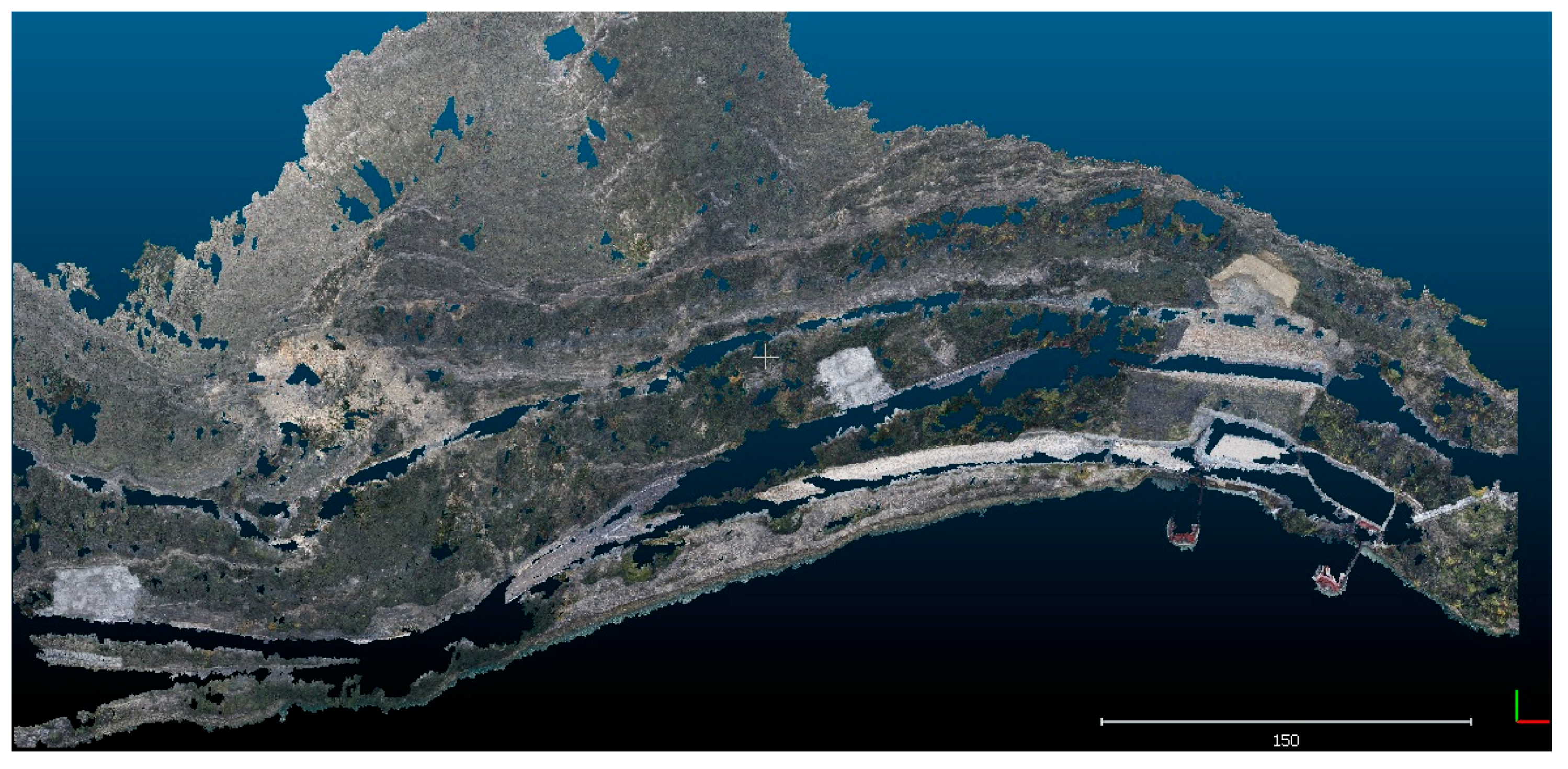
A first observation that can be made by seeing the two point clouds, is that the final 3D point cloud (Figure 14) does not present so many holes. The MMS allowed to acquire the elements close to the path followed along the road and to compensate for the gaps that had been created in the CRP point cloud.

This explains that a possible combination of different surveying techniques, their different use and the different data acquired can be complementary and guarantee a complete mapping of the same site of interest. The previous statement is true as far as both the RMSE and the standard deviation are small. Besides the integration between CRP and MMS, we also computed the accuracy evaluation between the aligned MMS point cloud and the photogrammetric control points on natural features. As explained in Section 3.1, the EDM technology system is based on pillars for control and spherical targets for checking the photogrammetric accuracy. Once the quality of the photogrammetric survey has been confirmed, photogrammetry can also be used for checking the accuracy of the MMS based on natural features. Taking the 22 check points of the CRP solution as a reference, we computed the distance on three natural check points (randomly combined) doing a point-pair registration. As shown in Figure 15, the error value is subdecimeter and comparable to the distance evaluation between CRP and MMS point clouds.

6. Discussion

The experiments presented above involved point clouds produced with CRP and MMS solutions. The experiment was designed to investigate whether MLS can reach a degree of accuracy to complement CRP for mapping monitored areas; it was motivated for understanding the potential of an innovative acquisition method using MMS in challenging environments.

The MMS proved to be very useful due to the rapidity of acquisition and the ease of use. In the presence of an existing reliable photogrammetric survey, the mobile mapping can be easily constrained, reducing the post-processing actions required; the developed methodology made the combination with existing surveys very easy for expert operators. Kaarta Stencil 2 has a strong potentiality to generate a higher number of points when composing the 3D point clouds. The advantage of using the MMS at the ground level allows users to enrich the point cloud in areas difficult to acquire with the CRP from the other side, for example, the roads surface and objects hidden or covered by the crown of trees. It is clear that these geomatics technologies may be complementary to one another in creating complete high-quality fully 3D representations. Nevertheless, the noisy data invalidate their usefulness to create high accuracy 3D models of the area, complementary to the photogrammetric one undertaken in the previous campaigns.

This work demonstrates its usefulness for data acquisition and mapping purposes, presenting similarities with the case studies described in [3,13], referring to the hand-held use of MMS. Indeed, we have been able to manage the occlusions, which are unavoidable from the photogrammetric model. Therefore, the information can be considered complementary to CRP for mapping the entire area, i.e., for a comprehensive survey. However, we have corroborated that the MMS is not robust enough to be used for monitoring complex sites such as this Corte de Pallás site. One promising approach is to integrate an accurate differential GNSS to the MMS solution.

It is fair, however, to highlight some drawbacks that emerged from this research. First of all, the point cloud cannot be exploited from scratch; in fact, further work of alignment was undertaken (as described in Section 4). The more the traveled survey distance extends, the more the drift error increases. The use of some constraints along the path should reduce the drift error. Despite MMS being designed with the main purpose of collecting 3D data without the need to register the point cloud further, this work proved that, the achievement of a result exploitable for mapping purposes relies upon the co-registration with an existing, and more accurate, point cloud. As the survey needs to be integrated with other data, accurate planning of the survey is required; in other words, it is not enough to just walk (see loop closure issue in Section 3.4) in order to improve the accuracy and facilitate the integration. Monitoring data need a submillimeter accuracy; as we reached an accuracy that is not comparable to the photogrammetric one (5.6 ± 2.3 cm), hand-held MMS as it is now implemented (without an accurate implementation of GNNS) cannot be considered suitable for such monitoring purposes. Nevertheless, it is very useful to complete the mapping of challenging areas in a fast, agile, and affordable way.

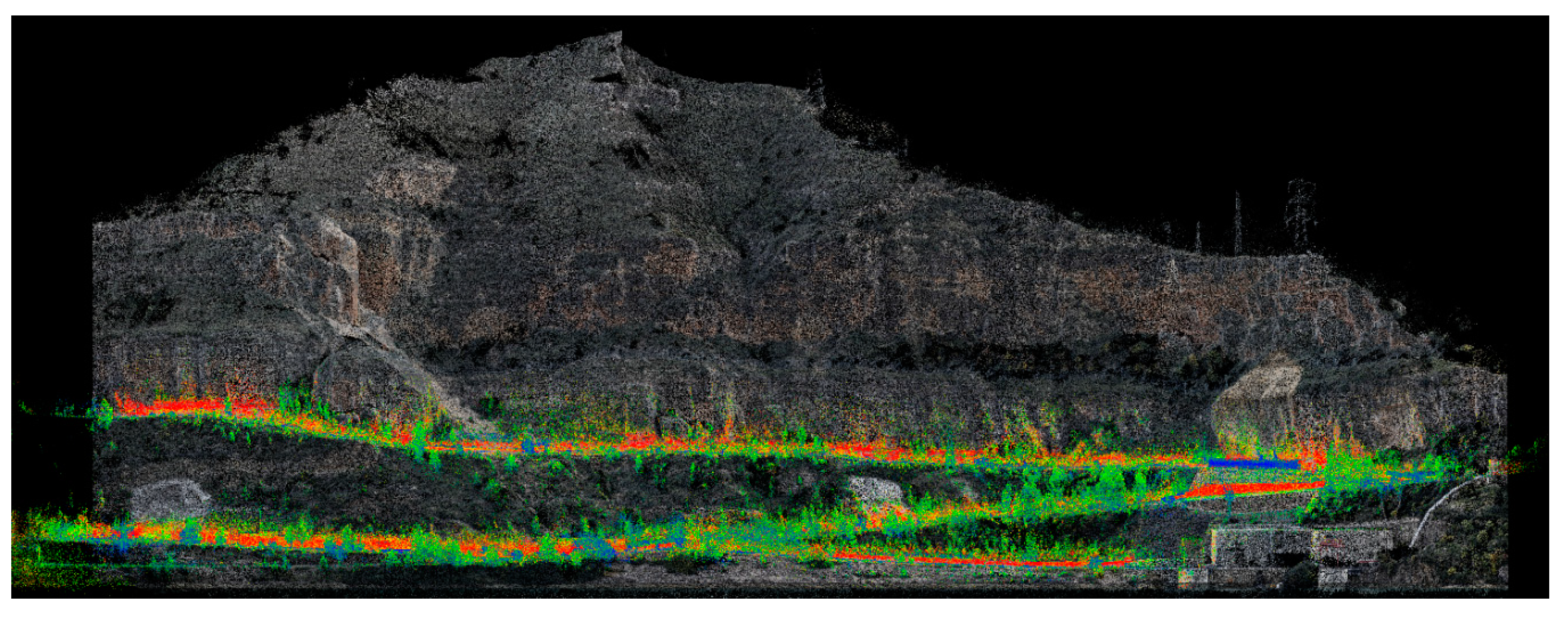
Another aspect that is worth discussing is the lack of RGB information. Indeed, the Kaarta MMS provides output 3D point clouds without the color information. This is an aspect that cannot be neglected, as environmental monitoring applications require in depth knowledge of a site. To overcome this limitation, the MMS cloud has been colorized, assigning the RGB values of corresponding neighbors from the CRP cloud. The colorized MMS cloud is depicted in Figure 16.

A final note is required with regard to the number of points that can be exploited with respect to the original raw data. As visible in Figure 13, to achieve a satisfactory accuracy comparable with the CRP one, the filtering steps brought to reduce the threshold up to values lower than 10 cm. This step increased the accuracy of the remaining points, at the expense of the number that was significantly reduced. In other words, due to the noise that is introduced by the tool, there is a waste of 3D information.

7. Conclusions

This research was aimed at assessing the use of hand-held MMS for environmental applications and, more in depth, for monitoring purposes. The case study investigated in Cortes de Pallas involved a very challenging area. The evidence that emerged from this study is that, as expected, CRP accuracy is strictly dependent on the supporting topographic network. Consequently, the MMS survey can only rely on it if combined in the same reference system. Once aligned, and in the case of the absence of UAV surveys, MMS was revealed to be an alternative to complete the 3D mapping of the area in a fast and agile way. As the management of occlusion is a well-known issue, often irresolvable even with a more sophisticated TLS system, the geomatic community should put more effort into improving the MMS accuracy and reliability.

As the Kaarta Stencil 2 is still under development and a growing number of new tools will enter the surveying market, this research is the occasion to set a useful baseline for further implementations demanded by the market, not only in civil engineering but also in building construction.