Energy-Based Prognosis of the Remaining Useful Life of the Coating Segments in Hot Rolling Mill

Abstract

The field of prognostic maintenance aims at predicting the remaining time for a system or component to continue being used under the desired performance. This time is usually named as Remaining Useful Life (RUL). The current study proposes a novel approach for the RUL estimation of coating segments placed on a hot rolling mill machine. A prediction method was developed, providing real-time updates of the RUL prediction during the rolling milling process. The proposed approach performs energy analysis on measurements of segment surface temperatures and hydraulic forces. It uses nonparametric statistical processes to update the predictions, within a prediction horizon/window, indicating the number of remaining products to be processed. To assess the probability of failure within the defined prediction window, Maximum Likelihood Estimation is used. The proposed methodology was implemented in a software prototype in the MATLAB environment and tested in an industrial use case coming from a steel parts manufacturer, facilitating testing and validation of the suggested approach. Real-world data were acquired from the operational machine, while the validation results support that the proposed methodology demonstrates reasonable performance and robustness against product type variations.

1. Introduction

A continuous evolution concerning the methods for manufacturing high added value products is taking place nowadays, aiming to raise productivity rates and product quality, as well as reduce the number of defected products. The adoption of efficient maintenance strategies is a key element for manufacturing industries, as they cannot afford to perform corrective maintenance actions as soon as they have a critical failure (run-to-failure strategy). Maintenance is important from an economical point of view, since in many industrial plants the maintenance costs often exceed 30% of the operational costs. The occurrence of unscheduled maintenance in manufacturing industries can introduce costly delays and breakdowns if the problem cannot be rectified on time [1]. Furthermore, manufacturers cannot rely only on time-based preventive maintenance, since its results are vulnerable to unexpected variations in process parameters that are related to tool and machine conditions, material quality, and human intervention, affecting the effectiveness of such maintenance techniques. Such static approaches could end up with replacing parts that are still in good condition, or, on the other hand, they could result in unexpected failures. However, predictive maintenance strategies can be deployed for in-advance determining the needs and driving suitable maintenance activities. The expected outcomes of predictive maintenance in manufacturing processes include optimized part usage, reduced costs, increased machinery lifetime, and improved product quality [2]. In the context of Industry 4.0, predictive maintenance (PdM) strongly relies on the Internet of Things (IoT) for timely data exchange. IoT-enabled PdM is attracting considerable investment from industries nowadays [3].

The problem of Remaining Useful Life (RUL) prognosis for tool components in manufacturing is important as prompt wear condition identification may lead to a reduction of downtime costs, lifetime increase, a better quality of surface finishing, and pre-scheduling of maintenance activities. Therefore, RUL estimation is straightforwardly correlated with tool-condition monitoring (TCM), since, although degradation is a non-stationary process, it is gradual [4].

Several approaches have been released within the last two decades, including implementations with machine learning (ML) methods, such as neural networks (NNs) systems, as well as based on mathematics–physics models. However, no general solution has been deployed yet. Irregular production conditions and non-stationary phenomena during production processes (e.g., cutting/rolling speed variations and production pauses) cause ML systems to face difficulties in providing such a generalized solution. However, the wide range of predefined methods and training algorithms throughout the literature has made them popular. On the other hand, approaches based on mathematics–physics models look more appropriate for production non-stationarities. Nevertheless, feature-selection along with the identification of the appropriate models and analysis procedures remains challenging.

The aim of this paper is to present a data-driven methodology for RUL estimation for the coating segments of a hot rolling mill that processes two different types of trailing arms. A prototype prediction software was designed and developed, to provide interval RUL estimations in terms of remaining products to process without quality degradation. The main contributions of this work are as follows: (1) the development of a novel method for the prediction of RUL in hot rolling milling machines that process different types of products, (2) the implementation of the RUL prediction method in a software prototype that enables the application in real industry cases and provides a graphical user interface for interacting with end-users, and (3) the evaluation of the method in an industrial case based on historical datasets. The results have shown that the method provides accurate predictions promptly. Since the proposed method is automated and can provide condition information without requiring specific skills or specialization from a maintenance operator, it could be used to improve the interaction of humans with automation technologies for supporting predictive maintenance and production sustainability, and essentially close the gap for the forthcoming Industry 5.0 paradigm. Although predictive maintenance solutions, such as the one presented in this work, are IoT solutions that may introduce new vulnerabilities for cyber-attacks in an industrial environment, cybersecurity has not been investigated in this work.

The remainder of this paper is organized as follows: Section 2 reviews the literature of condition monitoring and RUL prognostics in the context of cyber–physical production systems and predictive maintenance. Section 3 gives the theoretical framework behind the suggested approach. Section 4 describes the method’s implementation, while Section 5 includes a detailed description of the case study and presents the method’s validation. The conclusions of the study and suggestions for future work are summarized in Section 6.

2. Literature Review

2.1. Cyber–Physical Production Systems

The recent advances in information and computing technologies have resulted in a new industrial revolution, commonly referred to as the fourth industrial revolution, or Industry 4.0. This has introduced new practices and better service activities in the sphere of industrial production [5], while also establishing new initiatives, such as cyber–physical systems (CPSs), converting factories into intelligent, and reconfigurable systems [6]. Cyber–physical systems are systems that collaborate computational entities which are in intensive connection with the surrounding world and its ongoing processes, providing and using data-accessing and data-processing services available on the internet [7]. In other words, CPSs utilize sensors and actuators to make decisions based on their intelligence [8,9]. Hence, manufacturing or production processes can include hardware interfaces and computational software [8] to make decisions, communicate, and interact with humans (human-to-machine) or other machines (machine-to-machine) via communication channels. Apart from CPSs, innovations such as the Internet of Things (IoT), cloud computing (CC), and Big Data have enforced industries to take advantage of these technologies for successfully facing the recent changes in economic, social and environmental requirements. These developments have resulted in companies with networked assets producing a massive amount of data [2]. For useful data provision, cloud-based solutions are required [10,11], while the IoT is the key enabling technology for machine-to-machine interaction [3]. Communication between hardware, software, and other devices is usually described under the term “connectivity”. The expectations of CPSs include robustness, autonomy, self-organization, self-maintenance, self-repair, and efficiency [7].

2.2. Predictive Maintenance

The availability of massive data brings new opportunities for evolving maintenance practices. In networked factories, new technologies permit operators (or even intelligent systems) to monitor the machinery conditions. This has led to the investigation of PdM strategies. In the Industry 4.0 context, PdM strongly relies on IoT communications. IoT satisfies timely and correct information exchange, which is critical for the safe and effective behavior of the monitored components. An example of an industrial IoT solution that allows advanced PdM applications is presented in Civerchia, Federico et al. [12].

Predictive maintenance assumes that the monitored machine parts go through a measurable process of degradation, hence enabling the estimation of temporal windows for carrying out repair operations [2,13]. PdM comes to benefit from technological advances and predict the RUL of components through degradation measuring. Some examples of computer models for PdM in manufacturing nowadays include Auto-Regressive Integrated Moving Average (ARIMA) models for non-stationary processes, condition-based maintenance techniques [1], as well as Prognostics and Health Management (PHM), approaches using physics-based representations and analysis [14].

2.3. Methods for Assessing RUL

Tool prognostics, especially the RUL evaluation, and condition/wear monitoring have been widely investigated within the last two decades. Many approaches use features extracted from vibration data, force measurements, acoustic emission, and/or current signals [15]. The applied methods can be divided into two main categories: (1) data-driven methods, which utilize computational intelligence techniques, such as Machine Learning (ML); and (2) model-based methods, using mathematics/physics-based models to perform data analysis through statistical processes.

Several ML approaches for tool-wear monitoring and tool-condition identification have been released during the last two decades [4,16,17,18,19,20,21,22,23,24,25,26,27,28,29]. A monitoring strategy establishing a combination of four static and two dynamic NNs was presented by Scheffer et al. [4]. The static NNs were trained via the incremental Self-Organizing Map (SOM) algorithm, whereas the dynamic ones were trained with the Particle Swarming Optimization Algorithm (PSOA). This formulation has the advantage that the dynamic NNs can follow any development of wear, whereas protecting the monitoring system from possible data disturbances. Another technique was proposed by Scheffer and Heyns [16], which uses a series of NNs: one dynamic that is trained online with the PSOA method and four static that are trained offline with Levenberg–Marquardt back-propagation. Chen et al. [17] addressed several data fusion methods to extract features to use as input data for neural networks (NNs). The Index Multiplication Group (IMG) and the Indices Multiplication and Division Group (IMDG) fusion methods were found to be promising. In Haber and Alique [18], an artificial neural network (ANN) using a neural network output error (NNOE) model for predicting tool wear in machining process was tested, but the attempt was characterized by lack of diagnosis capability and inconsistency with process variations.

In more recent ML approaches, an approach was released by Wu et al. [19], making use of the random forest algorithm. Experimental results have shown that the random forest algorithm can generate very accurate predictions. Amongst the most popular ML methods are the approaches that make use of fuzzy logic systems [20,21,22,23], such as the Adaptive Network Fuzzy Inference System (ANFIS) [20] or the Neuro-Fuzzy Network (NFN) [21]. Fuzzy logic systems appear to have great accuracy for tool-condition monitoring (TCM) in milling processes, but they are characterized by big computational times, affecting negatively their applicability for online monitoring. Support Vector Machines (SVM) are also popular ML alternatives [20,24,25,26,27]. SVMs exhibit more moderate accuracy compared to FL methods, but they are much faster and more suitable for online tool life prediction. A multisensor global feature extraction method has been researched in Zhou and Xue [28]. A Kernel-based Extreme Learning Machine (KELM) executes the monitoring model, and a modified genetic algorithm (GA) is implemented to search the optimal parameter combinations in a two-objective optimization model. It was found that the overall error of the predicted tool wear was small. Although ML techniques are widely used nowadays in milling processes, many of the most promising methods are difficultly adaptable in real industrial operations, due to insufficient generalization capabilities for different manufacturing process conditions. However, in 2020, Ou et al. [29] suggested a novel TCM approach based on order analysis (OA) and stacked sparse auto-encoder (SSAE), which was applied in actual industrial manufacturing data and appeared to outperform the most methods which utilize neural networks in varied manufacturing conditions.

On the other hand, the methods of the second category aim to measure several parameters that are indirectly correlated to tool performance and use statistics or physics models to estimate tool wear. Five methods were tested in Rother et al. [30] for strip rolling mills, namely short-time Fourier transform (SHFT), continuous wavelet transforms (CWT), discrete wavelet transforms (DWT), Wigner–Ville distribution (WVD), and empirical mode decomposition (EMD), for detecting specific system fault states. The CWT, DWT, and EMD methods exhibited good applicability in non-stationary signals. From these three, CWT appeared to have the highest computational requirements, whereas DWT has the lowest, and EMD’s computational load is considered as the medium. The EMD method has the highest resolution of these three methods. In Yamaguchi et al. [31], cutting forces and acoustic emission (AE) signals are used for cutting-tool life estimation. Wear-state identification is based on a spectral exponent. The approach has shown effectiveness for timely warning when the tool is nearing the end of its life due to wear, as the spectral exponent becomes greater than 1. Other studies released, include Bayesian-filter-based [6] and Hidden Markov models [32]. In Lamraoui et al. [33], cyclostationarity was applied to vibration acceleration signals. This study aimed to extract efficient features for tool wear monitoring in a hot rolling mill. It was shown that the synchronous angular statistic (average and variance, Kurtosis, integrated Wigner–Ville spectrum) methods express cyclostationarity at first and second order. Moreover, parameters, namely kurtosis, power, spectral correlation function, and Wigner–Ville spectrum, are efficient for early diagnosis of faults in high-speed machining, compared with the traditional stationary methods. In Chi et al. [34], vibration signals were decomposed through ensemble empirical mode decomposition (EEMD), and the intrinsic mode functions (IMFs), frequency spectrums of IMFs, and features related to amplitude changes of frequency were obtained. An algorithm was developed for real-time estimation of tool wear. The method proved to be very effective, with very low root mean square error. In Stavropoulos et al. [35], third-degree regression models were used for vibration and electrical current signals. It was found that tool-wear estimation predictability is affected by the mean vibration signal energy, while electrical current signals provided clearer prediction results.

A point at which ML outweighs model-based methods is the availability of predefined NNs, fuzzy-logic systems, and learning algorithms throughout the international literature. On the other hand, methods based in mathematics/physics models require one to build a model and develop the analysis process on his/her own, specialized for the case study. However, ML techniques face difficulties in dealing with production non-stationarities (e.g., processing parameter variations, production pauses), and most of the existing ML methods only carry out with constant working conditions. In contrast, model-based methods do better in that section. Managing production non-stationarity is a key aspect for generating a good prognosis, as adapting to condition changes is necessary for detecting changes in the increase rate of wear. The approach described in this study is classified in the second category of methods. Considering tool wear as a result of material fatigue due to thermomechanical load alternations, the method uses a novel feature to model tool wear and generates prognosis using a mathematical framework. The feature is constructed by performing energy analysis [36] on force and temperature data.

In rolling mills, PdM techniques are nowadays implemented instead of traditional break-down or preventive maintenance strategies [37]. The majority of research studies concern fault detection in roller bearings, gearboxes and drivetrains, the tilting table, drivers, or the hydraulic systems [38,39,40,41,42,43]. Although there are studies for condition monitoring in rollers [44,45], no work was found dealing specifically with the coating segments, for which this paper’s method is applied. The method’s effectiveness was examined through nine Monte Carlo tool-replacement prediction simulations on real data. The performance was evaluated in terms of mean absolute percentage error (MAPE), a commonly used measure of accuracy in forecasting. The proposed method leads to timely warning for tool failure, deals well with production non-stationarities, and provides an effective and highly accurate alternative for TCM, RUL prognosis, and predictive maintenance.

3. Approach

3.1. Problem Definition

The approach presented in this work aims at enabling PdM in a hot rolling milling machine. The model of the rolling milling machine is presented in Figure 1. The rolling mill machine is composed of two rolling cylinders which rotate with the use of torque motors. The lower rolling cylinder has a fixed position and only the upper cylinder can move linearly (vertical), as shown in Figure 1. Each cylinder contains some coating segments. The segments have a wear-resistant coating that degrades over time. The segments’ coating degrades due to the forces, friction, and high temperatures during the process. At the end of their useful life, the segments are replaced with exactly similar segments in terms of geometry and material. However, in the problem under study, since they are replaced with identical spare parts, the dimensions of the segments are not considered as parameters of the problem and do not have a contribution to the RUL estimation method.

In many cases, the coating thickness cannot be measured during production, so an indirect measurement must be applied to indicate their wear. For this reason, temperature and hydraulic force sensors are placed on the rolling mill, and the measurements are stored in a database. The analysis of the acquired data for RUL estimation is the main target of this study.

In particular, this study discusses on an energy-based RUL estimation methodology based on the assumption that each product that is loaded on the rolling mill machine charges the working tools with an excitation dynamic energy, resulting to machine segments wear. As segment usage is quite short-term in this use case (approximately 15 days), corrosion phenomena due to oil supply in the rolling cylinders do not affect segment wear significantly. Thus, tool fatigue is mainly dependent on each product’s energy contribution to degradation, resulting in the product’s contact with the segments. After the product is processed, the tool’s remaining embodied energy capacity decreases.

3.2. Method for RUL Prediction in Hot Rolling Mills

The flow of the proposed approach is presented next, in Figure 2:

Figure 2 shows that, in real-time and while the manufacturing process is underway, RUL (remaining products to proceed) is calculated based on the following:

• The remaining embodied energy capacity of the segments.
• The mean rate of wear progress.

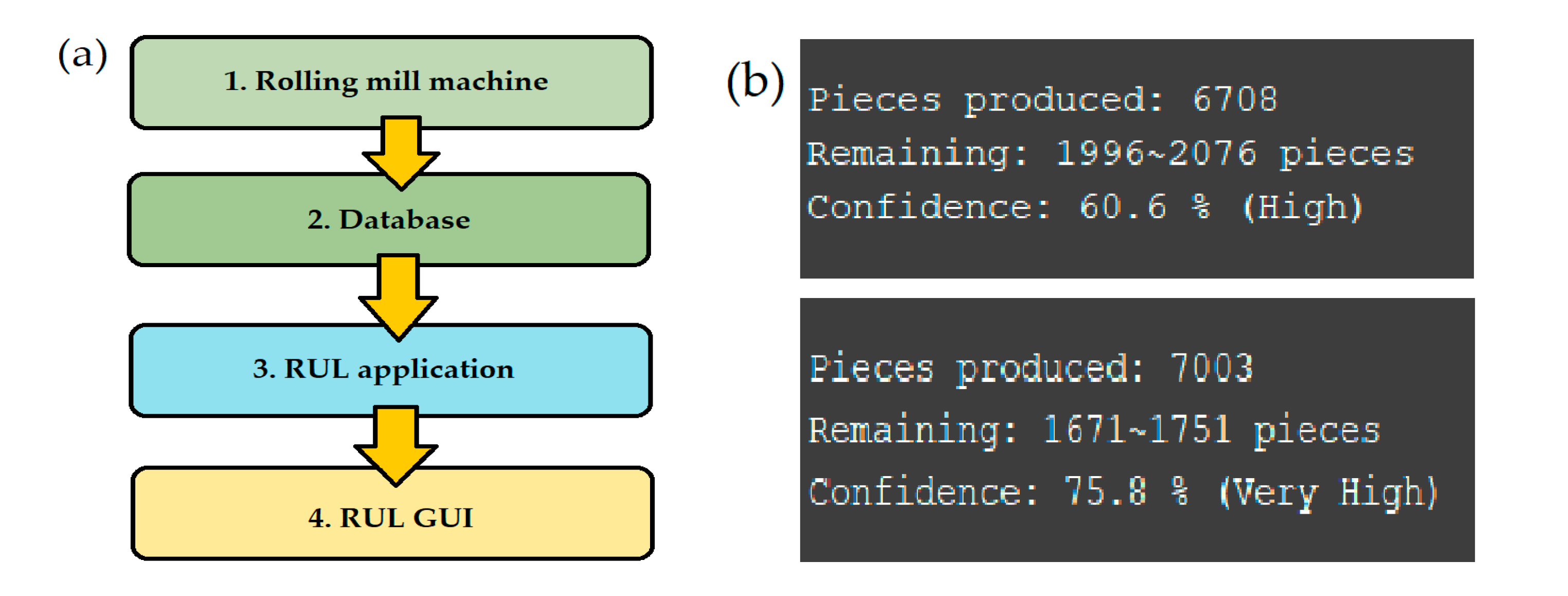
In this case, RUL calculates the remaining products that can be produced before the coating of the segment reaches its useful life.

Under the assumption that someone a priori had decided to change the segments when they reach a certain wear stage, this energy level is considered as the segments’ embodied energy capacity. Tool breakage could also be selected as the aforementioned wear stage. The embodied energy capacity is calculated from past sensor data (baseline/historic data), measuring key parameters that affect wear and converting them into energy concentration. For each baseline session, the concentrated amount of energy from the beginning of usage of the segments until their replacement is calculated. Due to data disturbances (e.g., floor vibration from nearby machinery) [15], the baseline energies will probably have a small variance. The mean of the baseline energy values is defined as the tools’ embodied energy capacity. The number of baseline sessions is defined such that the variance of the baseline energies is low enough.

A feature representing the excitation energy from each processed product is constructed in real-time from the normalized force (F) and temperature (T) measurements. Normalization is performed by removing the data mean from the data values and then dividing with their standard deviation. After performing an energy analysis [36] on these two time-series for each machine’s cylinder, we found that each cylinder’s excitation energy is as follows:

$$W=\underset{f_a}{\overset{f_b}{{\displaystyle \int }}}{G}_{FF}\left(f\right)df+\underset{f_a}{\overset{f_b}{{\displaystyle \int }}}{G}_{TT}\left(f\right)df-\underset{f_a}{\overset{f_b}{{\displaystyle \int }}}|G_{TF}\left(f\right)|df$$

(1)

where f is the frequency in Hz; G_FF(f) and G_TT(f) are the Power Spectral Densities (PSDs) of the normalized signals F and T, respectively; and G_TF(f) is the cross-PSD between F and T. In Equation (1), the term that contains the cross-PSD of F and T is removed to remove the part of T that is due to (“linearly” explained by) F. It should be noted that W is a mathematical quantity that is proportional to the energy that the processing of each product adds to the system. The norm in the last term is used because the cross-PSD part is a complex function of frequency. Integration boundaries f_a and f_b are defined by the acquired signals’ bandwidth. For a sampling frequency f_s, according to Shannon theorem, the maximum frequency in which signal information can be accessed is f_b = f_s/2. The lower integration frequency, f_a, is determined from the sensor’s specifications. It is the lowest band that the sensor can record data information. Energy W is calculated after the end of the processing of each product, and it is added to the already stored energy of the measuring cylinder, reducing the remaining capacity of its segments.

The next step is to estimate the mean rate of wear progress. The mean rate of wear progress is the mean added energy from each product that would result in the same product size as in the present period. This is calculated in Equation (2). The values of each product’s energy contribution W are collected, forming a sample that is real-time updated after the machine finishes each product’s processing.

$$E\left(\frac{dW}{dN}\right)=\frac{d\overline{W}}{dN}\approx \frac{\Delta W}{\Delta N}=\frac{\Sigma W}{N_t}$$

(2)

In Equation (2), N_t is the number of completely processed products, E is the mean value operator whereas the upper hyphen also stands for mean value, ΔW stands for the increase of the embodied energy in the system, ΔN is the increase of the number of fully processed products, and ΣW the total excitation energy stored (the sum of the energy contributions W of the products produced so far). The mean rate of wear progress is continuously updated as the production procedure goes on.

Given the embodied energy capacity (W_p) of the tool (or a group of tools depending on the case study structure), which has been offline estimated in the baseline phase, the remaining life is estimated as the number of pieces that are predicted to be processed until segment exchange. The RUL prediction N is calculated via the following equation:

$$N=\lfloor \frac{W_p-W_N}{{\left(\frac{d\overline{W}}{dN}\right)|}_{N=N_t}}\rfloor$$

(3)

where W_N is (equally to ΣW mentioned in Equation (2) the total energy added from the previously processed products, and N_t is the number of fully processed products. $\lfloor x\rfloor$ symbolizes the “floor” under x, i.e., the greater integer less or equal to x. This is because the RUL value must be an integer. To have a more flexible prediction, a constant prediction tolerance of ∓ΔN pieces is applied to the discrete RUL prediction N. The prediction is then transformed into a closed interval, defined shown as below:

$$\{\begin{array}{c}\left[N-\Delta {\rm N},{\rm N}+\Delta {\rm N}\right] , {\rm N}-\Delta {\rm N}>0\\ \left[0,N+\Delta {\rm N}\right] , {\rm N}-\Delta {\rm N}\le 0\end{array}$$

(4)

The procedure described up to Equation (4) is performed to each cylinder separately. The machine’s final RUL forecast interval is the lower RUL interval among these two.

The interval prediction described in the mathematical format (4) is valid if and only if the mean rate of wear progress lays inside the open interval (W1, W2):

$$W1=\frac{W_p-W_N}{N+\Delta N+1} , W2=\{\begin{array}{c}\frac{W_p-W_N}{N-\Delta {\rm N}-1} , {\rm N}>\Delta {\rm N}+1\\ \infty , N\le \Delta {\rm N}+1\end{array}$$

(5)

The probability of the RUL interval prediction to be verified is computed by assuming a normal distribution for the mean rate of wear progress, integrating the distribution from W1 to W2.

$$C=\underset{W2}{\overset{W1}{{\displaystyle \int }}}f\left(\frac{d\overline{W}}{dN}|\mu , {\sigma }^2\right)d\left(\frac{d\overline{W}}{dN}\right)$$

(6)

The integral in Equation (6) is the confidence of the prediction for f (x|µ, σ²) being the normal probability density function. The distribution parameters are defined with the Maximum Likelihood Estimation (MLE) method [46]. The designed prediction system saves the updates of the mean rate of wear progress, each time a product leaves the machine, and makes use of an updates vector to re-apply the MLE. The applied RUL estimation software is designed to provide displayed comments in a User Interface (UI) for each prediction’s confidence. A confidence assessment scale is adopted, accompanied by the assigned confidence labels. The procedure described up to here is repeated continuously, until it is time for replacing the segments. The assigned confidence labels are presented in

Table 1. Prediction confidence assessment scale and assigned labels.

Confidence Score		Assigned Labels
100%	Sure prediction	“Maximum”
85%–99.9%	Extremely reliable prediction	“Extremely High”
70%–85%	Very reliable prediction	“Very High”
50%–70%	Reliable prediction	“High”
30%–50%	Moderate prediction	“Moderate”
<30%	Unreliable prediction	“Poor”

.

4. Implementation

Prototype software was implemented for running the proposed approach in real time. The implementation and evaluation were carried out by using the MATLAB^® R2019a environment in a 64-bit Windows^® 10 operating system. MATLAB^® is a proprietary multi-paradigm programming language and numerical computing environment developed by MathWorks, Inc. (Natick, Massachusetts, United States of America). The Symbolic Math Toolbox, the Signal Processing Toolbox, the Statistics and Machine Learning Toolbox, and the Statistics and Machine Learning Toolbox were acquired to execute the method and perform the MLE for prediction confidence assessment. The source code was wrapped into a standalone executable package that runs real-time prognostics in the machine. The standalone package also requires the Data Acquisition Toolbox for creating and managing the data acquisition interface. An illustration of the system’s architecture is presented in Figure 3a, while in Figure 3b, examples of the Graphical User Interface (GUI) indications are portrayed. The GUI shows how many pieces have been produced by the used segments, the interval RUL forecast, and the forecast confidence.

The RUL prognosis application is designed to run in a PC outside the rolling mill machine. It was developed for exclusive use in the study of the rolling mill machine. Data from the machine’s sensor are provided from a database. The application offers the option to change three parameters: (1) the allowable embodied energy capacity, (2) the update horizon, and (3) the prediction tolerance mentioned in Equation (4) of Section 3. All can be adjusted from a configuration file. In the configuration file, the user determines the energy/wear level that the industry wants to replace the segments. This user-tuned parameter should not be higher than the energy level that corresponds to segment breakage, since it will generate invalid predictions. In the second line, the update rate is defined. For instance, a horizon value of 1 will provide RUL prediction updates after every single processed product, while a value of 100 will provide updates after every 100 products. For the third configuration parameter, the prediction tolerance is defined. Value selection of this parameter is subjective for each use case and depends on how strict or lenient forecast is demanded. A very low prediction tolerance increases prediction uncertainty. On the other hand, a tolerance value that is too high may lead to earlier and long-hour vigilance for carrying out maintenance. Taking into account the net processing time of each product can help define prediction tolerance, and thus avoid these issues.

5. Industrial Case Study and Approach Validation

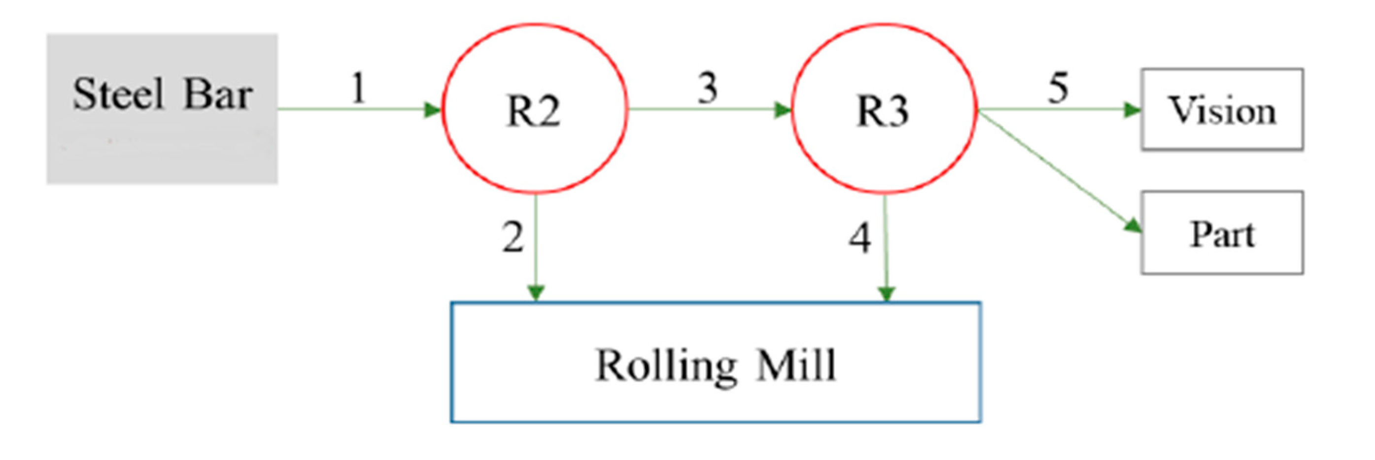
5.1. Manufacturing Process Description

The proposed approach was implemented upon the forming/pressing process of trailing arms through a rolling-mill-type machine. Predicting and scheduling the replacement of the coated segments aims at increasing, on the one hand, their lifetime and, on the other, increasing the trailing arms’ quality.

The rolling mill machine consists of two rollers. Each roller is supported at each side by twin-row spherical roller bearings. The bearings are lubricated either by oil circulation or with grease. The oil conducts away from the heat that enters via the rollers. Each cylinder contains three coating segments, accordingly to the layout in Figure 1 of Section 3.1. It is assumed that, at the end of their useful life, the segments are replaced with exactly similar segments in terms of geometry and material; therefore, their dimensions are not considered as parameters of the RUL estimation method.

The production line of the trailing arms starts by heating steel bars. After heating, the arms are inserted into a hot rolling mill for the forming/pressing process, before production goes on with the hardening process. The rolling mill process is carried out as shown in Figure 4. A robot (R2) picks up a heated metal bar (step 1) and proceeds with the rolling process (step 2). Another robot (R3) cooperates with the robot (R2) (steps 3 and 4), and once the rolling process has been completed, the steel bar is transferred from the robot (R3) for inspecting the geometry of the steel bar (step 5). Two different types of trailing arms are worked by the rolling mill and the processing of each arm lasts about 45 s.

5.2. Data Gathering and Preprocessing

The rolling mill machine has sensors on it that measure the temperature and hydraulic forces. The data used for the energy W estimation are (1) cylinder hydraulic forces in kNs and (2) segment surface temperatures in Celsius degrees. The diagram presented in Figure 5 depicts the data connections for the rolling mill machine. The data are collected from a total of four sensors implanted on the machine: two force and two temperature sensors on each cylinder. On the first level, the collected data from the hydraulic force sensors are stored to a local database in the motion controller and then transferred to a Programmable Logic Controller (PLC) database. The temperature data are directly stored in the PLC. The acquired data are transferred on a second level to the Historian database. The signals are transmitted in real-time into the processing PC via communication channels from the PLC database, once the processing of a single product has finished, to run the RUL estimation app. The incoming data are synchronized under common timestamps.

The historical data were used to validate our model. An example of data during a single trailing arm’s processing in the rolling mill machine is illustrated in Figure 6. There, the x-axis shows the processing time of the product, and the y-axis presents the hydraulic force (upper plot) and the segment surface temperature (lower plot). The collected data are being normalized before the execution of the proposed method. Normalization is performed by removing the data mean from the data values and then dividing them with their standard deviation (also see Section 3.2). Normalization is a mandatory process because data values must lie within a common numerical area, in order to avoid potential numerical problems.

5.3. Prediction Method Testing and Validation

The data values provided by the industrial company were grouped based on their timestamps, according to the format presented in

Table 2. A dataset sample.

Timestamp	Segment Top Surface Temperature (Celsius Degrees)	Segment Bottom Surface Temperature (Celsius Degrees)	Cylinder Hydraulic A Force (kilonewtons)	Cylinder Hydraulic B Force (kilonewtons)
2020-01-22T09:26:09	[189, 189, …, 102]	[548, 549, …, 90]	[−29, −16, …, −67]	[15, 3, …, −30]
2020-01-22T09:26:37	[262, 260, …, 158]	[542, 540, …, 527]	[−43, −49, …, −58]	[−18, 25, …, −24]
2020-01-22T09:27:03	[199, 198, …, 94]	[550, 550, …, 95]	[−46, −67, …, −61]	[−18, −9, …, −24]
2020-01-22T09:27:31	[256, 251, …, 147]	[548, 548, …, 496]	[−31, −17, …, −58]	[−2, 20, …, −34]
2020-01-22T10:28:43	[191, 187, …, 101]	[550, 550, …, 93]	[−46, −27, …, −61]	[−21, −6, …, −30]
2020-01-22T10:29:11	[260, 256, …, 157]	[544, 543, …, 536]	[−46, −21, …, −60]	[−21, −5, …, −24]
2020-01-22T10:29:37	[197, 195, …, 103]	[550, 550, …, 95]	[−58, −31, …, −61]	[−15, 13, …, −18]
2020-01-22T10:30:05	[259, 252, …, 152]	[550, 550, …, 511]	[−49, −24, …, −58]	[−21, −11, …, −34]
2020-01-22T10:30:33	[197, 194, …, 103]	[550, 550, …, 496]	[−16, −18, …, −61]	[12, 14, …, −36]

. There, the first column is the data timestamp, the second and the third refer to segment surface temperatures of the machine’s cylinders (top is for cylinder A and bottom is for cylinder B), and the last two refer to the hydraulic forces. Every two consecutive timestamps correspond to the processing of a single product.

Table 3. Data information.

Prediction Session	Start/End Dates and Timestamps
1	22/01/2020 (06:16)–29/01/2020 (13:24)
2	14/02/2020 (00:00)–19/02/2020 (01:14)
3	19/02/2020 (14:15)–24/02/2020 (06:38)
4	10/01/2020 (00:38)–14/01/2020 (11:38)
5	20/01/2020 (00:00)–20/01/2020 (23:59)
6	02/03/2020 (00:00)–17/03/2020 (06:35)
7	17/03/2020 (16:02)–23/03/2020 (19:16)
8	07/04/2020 (22:02)–12/04/2020 (16:52)
9	23/04/2020 (11:49)–23/04/2020 (13:16)

presents the different datasets that contain historical data captured during production and were used for validating the method. These provided data correspond to periods where no change of the coating segments had occurred, but do not correspond on the full duration of segment usage (from the time they were first mounted to the time they were replaced).

Each dataset corresponds to a different period, during which a specific set of six segments was used. Two different types and a different total number of trailing arms were processed during the periods captured by the available datasets. Moreover, a different number of trailing arms was processed in each captured period. To evaluate our approach, nine Monte Carlo prediction experiments were conducted, with each one using a single dataset as its input, to evaluate the prediction accuracy (output) of the discussed approach. In each prediction, the total energy that was absorbed from each cylinder is calculated and the higher of these two energies is considered as the dataset’s embodied energy capacity W_p. This capacity is assumed as the selected wear level for changing the segments for each distinct dataset. The objective of this validation strategy is to prove mathematically that the method’s prediction accuracy is independent of which wear level is selected as the replacing point of the segments so that the findings and the conclusions of the research are trustable. For performing the prediction experiments, the development of a specialized code in a software environment is required.

In the proposed approach, data PSD functions were estimated with Welch’s averaged periodogram, and numerical integration was performed via the trapezoidal method. The tolerance for constructing the RUL estimation interval was set to ΔN = ∓40 products. For the evaluation process, the prediction update horizon that is referred to in Section 4 was set to 1, to generate more predictions during the Monte Carlo experiments.

Indicative outcomes of prediction experiments are shown in Figure 7 and Figure 8. In Figure 7, the resulted segment wear from each product is indicated, in terms of added energy. The x-axis indicates the number of pieces that have been produced, and it is used as a discretization of time, and the y-axis shows the energy W that is added to each cylinder. Cylinder A refers to the upper cylinder of the rolling mill and cylinder B to the lower one. As it is shown in Figure 7, each processed trailing arm has a different energy contribution to segment wear, confirming the non-stationarity mentioned in Section 2. The statistical parameters of the added energy (mean, variance) change during the production timeline. Non-stationarity in wear exists because, in practice, it is impossible to attain the same processing conditions for each product.

In Figure 8, an indicative simulation outcome of the predictions is illustrated. The horizontal axis shows the number of produced products, while the vertical axis indicates the remaining products to be processed. The black line is the actual RUL value in remaining pieces to be processed, i.e., the number of products finally processed after each prediction update. Each dataset contains data for a specific period during which some trailing arm products were produced. The initial value of the actual RUL is the number of totally processed products during this period, and the final value is set to zero at the end of the period. Thus, the black line has a slope equal to −1. The red curves delimit the prediction interval updates, as they are estimated through Equation (4) of Section 3.2.

The accuracy of the proposed method was evaluated via the mean absolute percentage error (MAPE) [47]. The error of each prediction update is calculated based on the projected total production over the whole life of the machine’s segments. For example, when a discrete RUL prediction after N_t processed products is available and is equal to N, then the total production forecast of the segments from the start to the end of their use will be as follows:

$$N_{pf}=N_t+N$$

(7)

where N_pf is the total production forecast during the dataset, N_t is the number of products that have been completely processed on the time being, and N is the discrete RUL prediction in terms of remaining pieces to process (see Equation (3) in Section 3). As long as the actual total production of every simulation session is known before the simulation, the MAPE of each prediction simulation is calculated as follows:

$$MAPE=E\left(\frac{\left|N_p-N_{pf}\right|}{N_p}\right)$$

(8)

where E is the mean value operator, N_pf is the forecasted total production, and N_p is the actual total production during the dataset. The accuracy results of the nine Monte Carlo prediction experiments which were conducted to evaluate the proposed approach are presented in

Table 4. Accuracy results.

Prediction Session	MAPE	Accuracy (100%-MAPE)	Prediction Session	MAPE	Accuracy (100%-MAPE)
1	0.59%	99.41%	6	0.83%	99.17%
2	0.65%	99.35%	7	1.20%	98.80%
3	2.23%	97.77%	8	2.87%	97.13%
4	0.90%	99.10%	9	0.90%	99.10%
5	0.62%	99.38%

MAPE = mean absolute percentage error.

.

5.4. Discussion

Nine Monte Carlo predictions were performed to validate the proposed approach. Monte Carlo experiments are used to provide an interval estimation for an examined random variable, given a specified rate of reliability. Accuracy was considered as the examined variable in this case. Two different types of trailing arms were processed during the periods captured by the available datasets. Within a 99% confidence level, and according to Monte Carlo simulation theory [48], the accuracy of the method is, in general, estimated to be inside the open interval (98.11% and 99.49%). Independence among the MAPE and the maximum allowed embodied energy capacity (W_p) was examined via Pearson’s Correlation Coefficient. Covariance among them was measured equal to r_p ≈ 0.3, which interprets that accuracy is independent of which wear level is selected as the segments’ exchange point.

In parallel, prediction confidence estimation via MLE (described in Section 3) was performed at the same time with the Monte Carlo simulations. Plotting the confidence values of the interval RUL prediction during the trailing arms’ processing (see Figure 9 that corresponds to dataset 6, with x-axis indicating the number of produced products and the y-axis the prediction confidence), the evidence has shown that, in confidence levels between 30% and 50%, the success of the predictions was in a critical point in most cases. “In critical point” means that either the prediction interval fails but it is still close on the actual RUL value, or the prediction interval is marginally successful. Prediction confidence increases as the tools get closer to the end of their life. In extreme cases in which prediction confidence remains within the “moderate” status area for a very long time after the start of usage, it may be due to huge variations on production rhythm, or it may be implied that the data quality from the measurement system is not sufficient. Predictions with confidence higher than 50% can be taken seriously into account, while “moderate-level” confidence predictions should not pass indifferently, either.

Prediction confidence also depends on the applied tolerance of the constructed forecast interval. A higher tolerance amplitude leads to a higher validity of the predictions, but selecting a very high tolerance value might not make sense, as it will result in too lenient forecasts. In the current case study, the selection of an interval tolerance amplitude of plus/minus 40 pieces (equally an 80 product-long interval) results in having a prediction with a maximum replacement time declination around 1 h, since the processing of each trailing arm lasts about 45 s. This prediction interval is austere enough, so the selection of a higher tolerance amplitude would also be acceptable in the current case.

6. Conclusions and Future Work

In this study, a novel method was developed for RUL prognosis in the hot rolling milling process. The RUL estimation methodology was implemented in a software application, along with a method for estimating the confidence of the predicted RUL values. The proposed approach was validated in a case study in which two different types of trailing arms were produced by a rolling mill machine. The prediction capability of the method was evaluated based on historical datasets available by the manufacturing company, and the results indicate that the proposed method is accurate enough to be used in industrial practice.

Based on the experimental results, it can be supported that, by using this method, the industry can accurately—and according to the production plan—predict which day the maintenance activities have to be performed. Moreover, the method is characterized by robustness, since its performance is affected neither by product type variations on the machine nor by the user-tuned maximum accepted wear level that defines the tool replacement point.

Future work will focus on (1) enrichment of the proposed energy analysis approach to include additional parameters affecting segment wear, such as rolling speed or oil pressure measurements; (2) application in a real-world industrial environment together with a maintenance tasks scheduling tool; (3) application of the proposed approach in other industrial equipment, to assess its generality; and (4) investigation of cybersecurity aspects.

References

1. Efthymiou, K.; Papakostas, N.; Mourtzis, D.; Chryssolouris, G. On a Predictive Maintenance Platform for Production Systems. Procedia CIRP 2012, 3, 221–226. [Google Scholar] [CrossRef] [Green Version]
2. Ruiz-Sarmiento, J.; Monroy, J.; Moreno, F.-A.; Galindo, C.; Bonelo, J.-M.; Gonzalez-Jimenez, J. A predictive model for the maintenance of industrial machinery in the context of industry 4.0. Eng. Appl. Artif. Intell. 2020, 87, 103289. [Google Scholar] [CrossRef]
3. Compare, M.; Baraldi, P.; Zio, E. Challenges to IoT-Enabled Predictive Maintenance for Industry 4. IEEE Internet Things J. 2020, 7, 4585–4597. [Google Scholar] [CrossRef]
4. Scheffer, C.; Krätz, H.; Heyns, P.; Klocke, F.; Heyns, P.S. Development of a tool wear-monitoring system for hard turning. Int. J. Mach. Tools Manuf. 2003, 43, 973–985. [Google Scholar] [CrossRef]
5. Hozdić, E. Smart factory for industry 4.0: A review. Int. J. Modern Manuf. Technol. 2015, 7.1, 28–35. [Google Scholar]
6. Nikolakis, N.; Senington, R.; Sipsas, K.; Syberfeldt, A.; Makris, S. On a containerized approach for the dynamic planning and control of a cyber - physical production system. Robot. Comput. Manuf. 2020, 64, 101919. [Google Scholar] [CrossRef]
7. Monostori, L. Cyber-physical Production Systems: Roots, Expectations and R&D Challenges. Procedia CIRP 2014, 17, 9–13. [Google Scholar] [CrossRef]
8. Verl, A.; Lechler, A.; Schlechtendahl, J. Glocalized cyber physical production systems. Prod. Eng. 2012, 6, 643–649. [Google Scholar] [CrossRef]
9. Thiede, S.; Juraschek, M.; Herrmann, C. Implementing Cyber-physical Production Systems in Learning Factories. Procedia CIRP 2016, 54, 7–12. [Google Scholar] [CrossRef] [Green Version]
10. Uhlemann, T.H.-J.; Lehmann, C.; Steinhilper, R. The Digital Twin: Realizing the Cyber-Physical Production System for Industry 4.0. Procedia CIRP 2017, 61, 335–340. [Google Scholar] [CrossRef]
11. Nikolakis, N.; Alexopoulos, K.; Xanthakis, E.; Chryssolouris, G. The digital twin implementation for linking the virtual representation of human-based production tasks to their physical counterpart in the factory-floor. Int. J. Comput. Integr. Manuf. 2018, 32, 1–12. [Google Scholar] [CrossRef]
12. Civerchia, F.; Bocchino, S.; Salvadori, C.; Rossi, E.; Maggiani, L.; Petracca, M. Industrial Internet of Things monitoring solution for advanced predictive maintenance applications. J. Ind. Inf. Integr. 2017, 7, 4–12. [Google Scholar] [CrossRef]
13. Panicucci, S.; Nikolakis, N.; Cerquitelli, T.; Ventura, F.; Proto, S.; Macii, E.; Makris, S.; Bowden, D.; Becker, P.; O’Mahony, N.; et al. A Cloud-to-Edge Approach to Support Predictive Analytics in Robotics Industry. Electronics 2020, 9, 492. [Google Scholar] [CrossRef] [Green Version]
14. Aivaliotis, P.; Georgoulias, K.; Chryssolouris, G. A RUL calculation approach based on physical-based simulation models for predictive maintenance. In Proceedings of the 2017 International Conference on Engineering, Technology and Innovation (ICE/ITMC), Madeira Island, Portugal, 27–29 June 2017; pp. 1243–1246. [Google Scholar]
15. Mohanraj, T.; Shankar, S.; Rajasekar, R.; Sakthivel, N.; Pramanik, A. Tool condition monitoring techniques in milling process—A review. J. Mater. Res. Technol. 2020, 9, 1032–1042. [Google Scholar] [CrossRef]
16. Scheffer, C.; Heyns, P.; Heyns, P.S. An industrial tool wear monitoring system for interrupted turning. Mech. Syst. Signal Process. 2004, 18, 1219–1242. [Google Scholar] [CrossRef]
17. Chen, S.-L.; Jen, Y. Data fusion neural network for tool condition monitoring in CNC milling machining. Int. J. Mach. Tools Manuf. 2000, 40, 381–400. [Google Scholar] [CrossRef]
18. Haber, R.E.; Alique, A. Intelligent process supervision for predicting tool wear in machining processes. Mechatronics 2003, 13, 825–849. [Google Scholar] [CrossRef]
19. Wu, D.; Jennings, C.; Terpenny, J.; Kumara, S. Cloud-based machine learning for predictive analytics: Tool wear prediction in milling. In Proceedings of the 2016 IEEE International Conference on Big Data (Big Data), Washington, DC, USA, 5–8 December 2016; pp. 2062–2069. [Google Scholar]
20. Li, X.; Er, M.; Ge, H.; Gan, O.P.; Huang, S.; Zhai, L.; Linn, S.; Torabi, A.J. Adaptive Network Fuzzy Inference System and support vector machine learning for tool wear estimation in high speed milling processes. In Proceedings of the IECON 2012—38th Annual Conference on IEEE Industrial Electronics Society, Montreal, QC, Canada, 25–28 October 2012; pp. 2821–2826. [Google Scholar]
21. Zhang, C.; Yao, X.; Zhang, J.; Jin, H. Tool Condition Monitoring and Remaining Useful Life Prognostic Based on a Wireless Sensor in Dry Milling Operations. Sensors 2016, 16, 795. [Google Scholar] [CrossRef] [Green Version]
22. Ren, Q.; Balazinski, M.; Baron, L.; Jemielniak, K.; Botez, R.M.; Achiche, S. Type-2 fuzzy tool condition monitoring system based on acoustic emission in micromilling. Inf. Sci. 2014, 255, 121–134. [Google Scholar] [CrossRef]
23. Cuka, B.; Kim, D.-W. Fuzzy logic based tool condition monitoring for end-milling. Robot. Comput. Manuf. 2017, 47, 22–36. [Google Scholar] [CrossRef]
24. Cho, S.; Binsaeid, S.; Asfour, S. Design of multisensor fusion-based tool condition monitoring system in end milling. Int. J. Adv. Manuf. Technol. 2009, 46, 681–694. [Google Scholar] [CrossRef]
25. Sun, J.; Hong, G.S.; Wong, Y.; Rahman, M.; Wang, Z. Effective training data selection in tool condition monitoring system. Int. J. Mach. Tools Manuf. 2006, 46, 218–224. [Google Scholar] [CrossRef]
26. Wang, G.; Yang, Y.; Li, Z. Force Sensor Based Tool Condition Monitoring Using a Heterogeneous Ensemble Learning Model. Sensors 2014, 14, 21588–21602. [Google Scholar] [CrossRef] [Green Version]
27. Gao, C.; Xue, W.; Ren, Y.; Zhou, Y. Numerical Control Machine Tool Fault Diagnosis Using Hybrid Stationary Subspace Analysis and Least Squares Support Vector Machine with a Single Sensor. Appl. Sci. 2017, 7, 346. [Google Scholar] [CrossRef] [Green Version]
28. Zhou, Y.; Xue, W. A Multisensor Fusion Method for Tool Condition Monitoring in Milling. Sensors 2018, 18, 3866. [Google Scholar] [CrossRef] [PubMed] [Green Version]
29. Ou, J.; Li, H.; Huang, G.; Zhou, Q. A Novel Order Analysis and Stacked Sparse Auto-Encoder Feature Learning Method for Milling Tool Wear Condition Monitoring. Sensors 2020, 20, 2878. [Google Scholar] [CrossRef] [PubMed]
30. Rother, A.; Jelali, M.; Soffker, D. A brief review and a first application of time-frequency-based analysis methods for monitoring of strip rolling mills. J. Process. Control 2015, 35, 65–79. [Google Scholar] [CrossRef]
31. Yamaguchi, T.; Higuchi, M.; Shimada, S.; Kaneeda, T. Tool life monitoring during the diamond turning of electroless Ni–P. Precis. Eng. 2007, 31, 196–201. [Google Scholar] [CrossRef]
32. Vallejo, A.G., Jr.; Flores, J.A.N.; Menendez, R.M.; Sucar, L.E.; Rodriguez, C.A. Tool-Wear Monitoring Based on Continuous Hidden Markov Models. In Iberoamerican Congress on Pattern Recognition; Lazo, M., Sanfeliu, A., Eds.; Springer: Berlin/Heidelberg, Germany, 2005; pp. 880–890. [Google Scholar]
33. Lamraoui, M.; Thomas, M.; El Badaoui, M. Cyclostationarity approach for monitoring chatter and tool wear in high speed milling. Mech. Syst. Signal Process. 2014, 44, 177–198. [Google Scholar] [CrossRef]
34. Chi, Y.; Dai, W.; Lu, Z.; Wang, M.; Zhao, Y. Real-Time Estimation for Cutting Tool Wear Based on Modal Analysis of Monitored Signals. Appl. Sci. 2018, 8, 708. [Google Scholar] [CrossRef] [Green Version]
35. Stavropoulos, P.; Papacharalampopoulos, A.; Vasiliadis, E.; Chryssolouris, G. Tool wear predictability estimation in milling based on multi-sensorial data. Int. J. Adv. Manuf. Technol. 2015, 82, 509–521. [Google Scholar] [CrossRef] [Green Version]
36. Bendat, J.S.; Piersol, A.G. Random Data: Analysis and Measurement Procedures; Wiley: New York, NY, USA, 1986. [Google Scholar]
37. Tirpude, V.D.; Modak, J.P.; Mehta, G.D. Vibration based condition monitoring of rolling mill. Int. J. Sci. Eng. Res. 2011, 2, 1–10. [Google Scholar]
38. Yuan, J.; He, Z.; Zi, Y.; Liu, H. Gearbox fault diagnosis of rolling mills using multiwavelet sliding window neighboring coefficient denoising and optimal blind deconvolution. Sci. China Ser. E Technol. Sci. 2009, 52, 2801–2809. [Google Scholar] [CrossRef]
39. Chen, J.; Wan, Z.; Pan, J.; Zi, Y.; Wang, Y.; Chen, B.; Sun, H.; Yuan, J.; He, Z. Customized maximal-overlap multiwavelet denoising with data-driven group threshold for condition monitoring of rolling mill drivetrain. Mech. Syst. Signal Process. 2016, 68, 44–67. [Google Scholar] [CrossRef]
40. Farina, M.; Osto, E.; Perizzato, A.; Piroddi, L.; Scattolini, R. Fault detection and isolation of bearings in a drive reducer of a hot steel rolling mill. Control Eng. Pr. 2015, 39, 35–44. [Google Scholar] [CrossRef]
41. Deshpande, V.; Modak, J. Maintenance strategy for tilting table of rolling mill based on reliability considerations. Reliab. Eng. Syst. Saf. 2003, 80, 1–18. [Google Scholar] [CrossRef]
42. Xie, Z.-J.; Li, X.-J.; Chen, P. Design of an equipment condition monitoring and fault diagnosis network system for the main drive of a hot strip mill. J. Chongqing Univ. 2008, 11. Available online: http://en.cnki.com.cn/Article_en/CJFDTotal-FIVE200811003.htm (accessed on 27 September 2020).
43. Li, G.-Y.; Dong, M. A Wavelet and Neural Networks Based on Fault Diagnosis for HAGC System of Strip Rolling Mill. J. Iron Steel Res. Int. 2011, 18, 31–35. [Google Scholar] [CrossRef]
44. Yuan, G.; Wang, Y.; Liu, X. Real-time optical detection system for monitoring roller condition with automatic error compensation. Opt. Lasers Eng. 2014, 53, 69–78. [Google Scholar] [CrossRef]
45. Tang, Y.H.; Lin, G.X.; Zhang, C.L. Study of On-Line Condition Monitoring System for Roller Based on HMM. Adv. Mater. Res. 2010, 139, 2546–2549. [Google Scholar] [CrossRef]
46. Myung, I.J. Tutorial on maximum likelihood estimation. J. Math. Psychol. 2003, 47, 90–100. [Google Scholar] [CrossRef]
47. De Myttenaere, A.; Golden, B.; Le Grand, B.; Rossi, F. Mean Absolute Percentage Error for regression models. Neurocomputing 2016, 192, 38–48. [Google Scholar] [CrossRef] [Green Version]
48. Landau, D.P.; Binder, K. A Guide to Monte Carlo Simulations in Statistical Physics; Cambridge University Press: Cambridge, UK, 2014. [Google Scholar]
Figure 1. Industrial rolling mill with three segments at their end of operational life (red color) on cylinder B and three new (blue color). Cylinder A can move linearly in the vertical direction.
Applsci 10 06827 g001
Figure 2. Flowchart of the proposed approach.
Applsci 10 06827 g002
Figure 3. (a) Layered architecture of the implemented approach, (b) examples of RUL GUI indications.
Applsci 10 06827 g003
Figure 4. Rolling mill process.
Applsci 10 06827 g004
Figure 5. Data connections.
Applsci 10 06827 g005
Figure 6. Indicative data plots during the processing of a single trailing arm.
Applsci 10 06827 g006
Figure 7. Indicative added energy W time-series.
Applsci 10 06827 g007
Figure 8. A sample of prediction simulation outcome.
Applsci 10 06827 g008
Figure 9. Indicative confidence increase curve during a prediction simulation session.
Applsci 10 06827 g009