Article

A Taillight Matching and Pairing Algorithm for Stereo-Vision-Based Nighttime Vehicle-to-Vehicle Positioning

1
Department of Information Communication Convergence Technology, Soongsil University, Seoul 06978, Korea
2
School of Electronic Engineering, Soongsil University, Seoul 06978, Korea
*
Author to whom correspondence should be addressed.
Appl. Sci. 2020, 10(19), 6800; https://doi.org/10.3390/app10196800
Submission received: 17 July 2020 / Revised: 21 September 2020 / Accepted: 22 September 2020 / Published: 28 September 2020
(This article belongs to the Section Computing and Artificial Intelligence)

Abstract

:

Featured Application

This paper proposes taillight detection, stereo taillight matching, and taillight pairing methods for the stereo-vision-based nighttime vehicle-to-vehicle positioning process. This process can be used in advanced driver-assistance systems and autonomous vehicles.

Abstract

The stereo vision system has several potential benefits for delivering advanced autonomous vehicles compared to other existing technologies, such as vehicle-to-vehicle (V2V) positioning. This paper explores a stereo-vision-based nighttime V2V positioning process by detecting vehicle taillights. To address the crucial problems when applying this process to urban traffic, we propose a three-fold contribution as follows. The first contribution is a detection method that aims to label and determine the pixel coordinates of every taillight region from the images. Second, a stereo matching method derived from a gradient boosted tree is proposed to determine which taillight in the left image a taillight in the right image corresponds to. Third, we offer a neural-network-based method to pair every two taillights that belong to the same vehicle. The experiment on the four-lane traffic road was conducted, and the results were used to quantitatively evaluate the performance of each proposed method in real situations.

1. Introduction

Transportation is an essential factor in human lives, as it plays an important role in developing civilization. Therefore, recent work on both scientific and industrial sides has focused on constructing an intelligent transport system (ITS), in which autonomous vehicles are arguably the most attractive part [1,2,3]. It is partly due to the rapid development of artificial intelligent approaches that their contributions have been shown in several fields in recent years [4,5,6]. However, since the final target is completely replacing the traditional vehicles with the autonomous ones, there are still many challenges ahead that need to be resolved. For example, the on-road autonomous vehicles may need to estimate each other’s positions to maintain safe distances and make urgent decisions when necessary. Thanks to that, we can avoid traffic accidents and congestion. Therefore, there is an increasing demand for an efficient vehicle-to-vehicle (V2V) positioning solution.
Referring to previous studies, many drawbacks that affect the performances of the existing V2V positioning technologies, such as time difference of arrival (TDOA) and light detection and ranging (LiDAR), have been observed [7,8]. In particular, with TDOA, an estimation result greatly depends on the time measurement, which causes difficulty in obtaining high accuracy in practice. Besides, LiDAR has to face some major limitations such as high cost, complicated installation, high sensitivity to signal interference, and jamming. Compared to these methods, the stereo vision system has some strong points as follows. First, the stereo vision system has an affordable price. Second, it is easily installed and maintained on the vehicle. Third, the stereo vision system can observe the appearance of the objects. Therefore, the stereo vision system can be considered as an alternative for the V2V positioning application.
To estimate the world coordinates of the object relative to the camera using the stereo-vision-based approach, initially, this object has to be detected from the captured image. However, it is extremely difficult to directly detect a vehicle at nighttime, since the appearance of the vehicle may become hardly observable due to the inadequate lighting conditions. Instead, most papers focus on detecting the most prominent part of the vehicle at nighttime (vehicle lighting), which is often a taillight [8,9,10,11]. In these papers, they use the stereo vision system, which includes two cameras, on the host vehicle to capture a real scene from two different views. Next, the world coordinates of the front vehicle’s taillights can be determined based on the relation between their corresponding pixel coordinates on the two captured images. This helps in estimating the position of the corresponding front vehicle. However, as all of them were based on simulation experiments with a single in-front vehicle, they have not dealt with three serious problems that need to be addressed to locate multiple front vehicles in practice. First, in the urban traffic environment, the cameras would presumably capture several light sources in the front, which may lead to difficulties in identifying the real taillight. Second, with many taillights detected from each image, how can we determine which one in the left image corresponds to a certain one in the right image. The third problem is how to pair every two taillights that belong to the same vehicle so that the vehicle’s presence can be confirmed. These three issues, which are respectively termed the detection problem, the stereo matching problem, and the pairing problem, are what we want to address in this paper.
Initially, we briefly review what has been done in previous works to deal with each of the above problems as follows:
(1) Detection problem: Due to the arbitrary shape and size of a vehicle’s taillights, it is challenging based on these characteristics to detect the taillight regions from an image, especially in nighttime situations. The most popular approach is relying on color and brightness, given the assumption that the vehicle’s taillights dominantly contain red points and their brightness is relatively higher than the other parts of the image. Specifically, they consider the threshold based on different color spaces, such as HSV [12,13,14,15], Lab [16], Y’UV [17], grayscale [18], or RGB [19], and use some conventional techniques [12,13,15,16,17,18,19] or machine-learning-based techniques [14] to detect the taillights from the image. However, the previous works often lacked a step to verify whether the detected region is a taillight or just a bright object. Furthermore, most of them have not mentioned labeling and determining the pixel coordinates of each detected taillight region, which is mandatory for V2V positioning.
(2) Stereo matching problem: Stereo matching [20] is a well-known problem that has appeared in many computer vision studies. In particular, it involves the task of determining which part of one image corresponds to a particular part of another image. These two images are taken of the same real scene but from different viewpoints. Previous studies mostly resolved the stereo correspondence problem by proposing a dense matcher to compare each small patch between two images for depth estimation or 3D reconstruction [21,22,23,24,25]. These approaches have two major drawbacks. First, the stereo matching that operates on the full image may generate bad results on low textured or non-Lambertian surfaces. Second, since the regions of interest often just fill in a small part of the image, the dense stereo matching task will possibly lead to high computational complexity, which may affect the performance in a real-time application like V2V positioning.
(3) Pairing problem: Regularly, to decide whether the two taillights belong to the same vehicle, the common approach is comparing some relations relevant to their size, color, and position with some particular thresholds [12,13,14,15,16,17,18,19,26]. The threshold values are usually chosen empirically but must be reasonable to distinguish between the two taillights. Therefore, these methods lack the flexibility to handle different cases in real situations. Furthermore, many of them are applied for the surveillance camera [13,16,17,19,26], which has a different perspective from the vehicle-mounted camera used in our positioning system.
To solve the aforementioned problems, we propose three methods, which are summarized as a three-fold contribution below:
  • A detection method in which we derive a connected-component analysis algorithm to determine the region and estimate the pixel coordinates of each candidate taillight in the image. In this method, we also provide a rule-based verification phase to reduce the number of outliers in detection results as much as possible.
  • A stereo matching method that uses a gradient boosted tree classifier for ascertaining which taillight in the left image is the same as that in the right image, while the other part of the image, which is not the target for V2V positioning, is ignored. Thanks to that, we reduce the computational complexity when compared with the conventional stereo matching approaches.
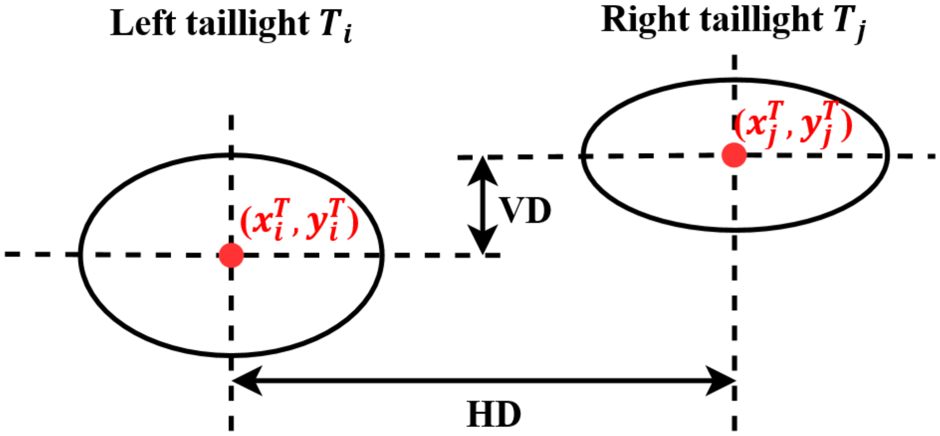
  • A neural-network-based pairing algorithm that adaptively determines the threshold of the horizontal distance, that of the vertical distance, and the correlation between two arbitrary taillights to decide whether they belong to the same vehicle. It is different from the existing works that set the threshold empirically.
Furthermore, an outdoor experiment was conducted to capture the images in a nighttime traffic environment. The obtained images were then processed using our proposed methods, to reveal the performances of these methods in real situations.
The remainder of this paper is structured as follows. First, in Section 2, we explain the stereo-vision-based nighttime V2V positioning process, which utilizes the stereo triangulation approach for estimating the world coordinates of the front vehicle using the pixel coordinates of its taillights. Second, three proposed methods for taillight detection, stereo taillight matching, and taillight pairing are respectively described in Section 3. Section 4 demonstrates our experiments in the real traffic scenario and evaluates the performances of the proposed methods on the captured images. Finally, we present the conclusions in Section 5.

2. Stereo-Vision-Based Nighttime V2V Positioning

A stereo-vision-based V2V positioning process in nighttime scenarios includes five stages. In stage (1), the proposed taillight detection method is applied to locate the region and pixel coordinates of each taillight in each image. In stage (2), a stereo matching method is applied to determine which taillight detected from the left image corresponds to which taillight detected from the right image; and a pairing method in stage (3) is to associate every pair of taillights that belong to the same vehicle on each image. When the pixel coordinates of each taillight in the left and right images have been determined, the world coordinates of this taillight can be calculated in stage (4). Finally, given the world coordinates of each pair of taillights, the world coordinates of the corresponding vehicle are estimated in stage (5). An overview of this process is presented in Figure 1.
In this study, our contribution includes three proposed methods for the first three stages from (1) to (3). Therefore, they will be described in detail in the next section. Besides, the intuition behind stages (4) and (5) is explained as follows:
In stage (4), the stereo triangulation approach [27] is utilized to determine the world coordinates of each detected taillight, given an assumption that the two cameras capture the images simultaneously. We denote P ( X , Y , Z ) as the world coordinates of the taillight P; O L ( u L , v L ) and O R ( u R , v R ) , respectively, as the pixel coordinates of the left and right cameras’ optical centers; and p L ( x L , y L ) and p R ( x R , y R ) as the pixel coordinates of P in the left and right images. Additionally, two cameras have the same horizontal focal length f x and vertical focal length f y , and the camera baseline is b. The stereo triangulation approach for taillight positioning is illustrated in Figure 2.
When considering two similar triangles, Δ P p L p R and Δ P O L O R , the Oz-axis value Z of the taillight P can be calculated using the following equations, given that all the mentioned coordinates are already known:
p L p R O L O R = b x L + x R b = Z f x Z ,
Z = f x b x L x R ,
After calculating Z, the two remaining values, X and Y, of the world coordinates of P can be identified:
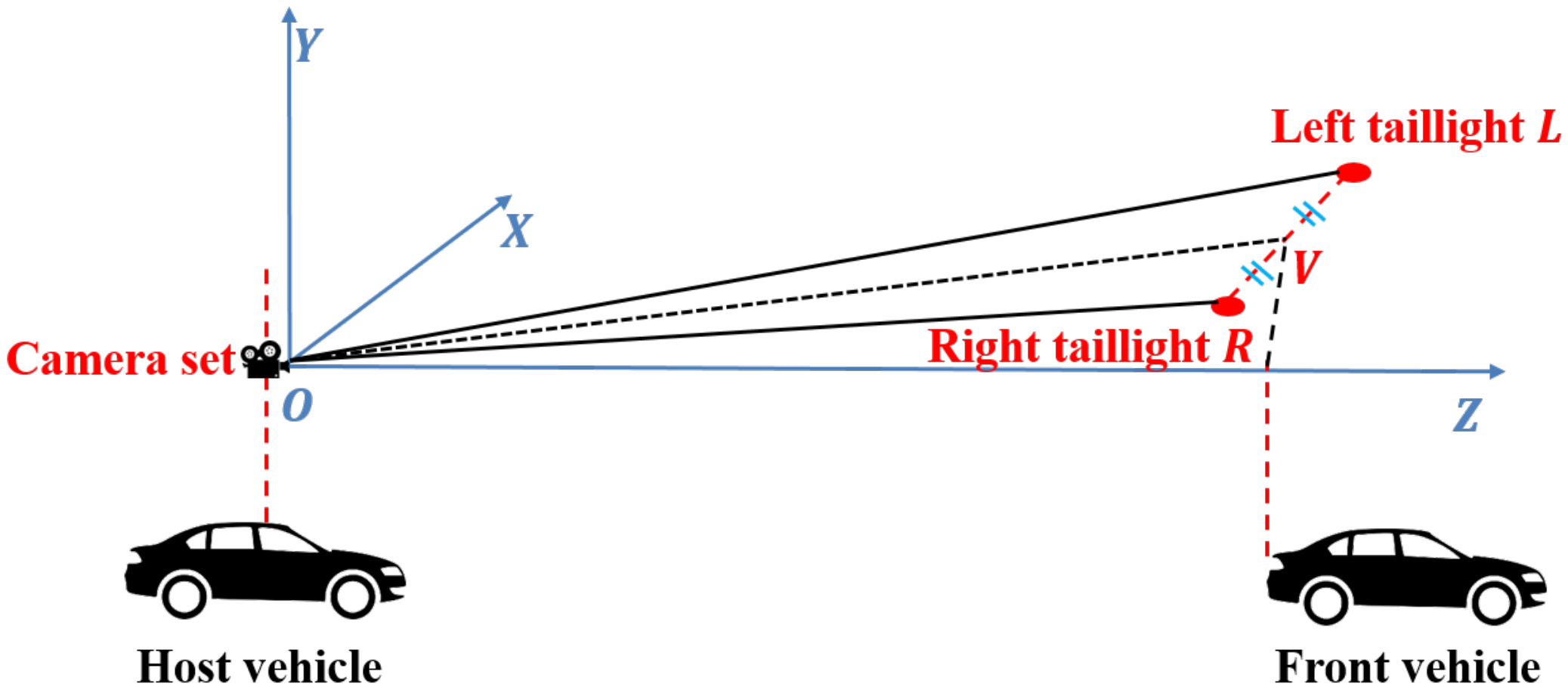
{ X = ( x L u L ) Z f x Y = ( y L v L ) Z f y ,
In stage (5), we suppose that V is the midpoint of the line segment that connects the left taillight L and right taillight R of the vehicle. The world coordinates of V can be considered as the position of the vehicle, as illustrated in Figure 3.
Once the world coordinates of the left taillight L and right taillight R have been determined as P L ( X L , Y L , Z L ) and P R ( X R , Y R , Z R ) , respectively, the world coordinates V ( X V , Y V , Z V ) of the front vehicle are given by:
{ X V = X L + X R 2 Y V = Y L + Y R 2 Z V = Z L + Z R 2 .

3. Proposed Methods

In this section, three proposed methods, including taillight detection, stereo taillight matching, and taillight pairing are respectively presented in Section 3.1Section 3.3.

3.1. Taillight Detection

In the V2V positioning context, the taillight detection stage aims to obtain the pixel coordinates of each taillight in the image. Moreover, the regions of these taillights need to be preserved because they will be further used in stereo taillight matching and taillight pairing stages. To accomplish these requirements, we propose a taillight detection method that includes two phases: generation and verification. The generation phase is to generate the candidate taillight region from the image. This phase comprises of three steps: HSV color thresholding, interesting point enhancement, and candidate region clustering. The verification phase, which consists of one step that is taillight verification, is to verify whether each candidate region is a taillight or not. The verification phase is an additional phase when compared with many existing detection methods [12,13,15,16,17]. It should be noted that sometimes when taillights from different vehicles approach each other, taillight occlusion occasionally occur under the camera’s viewpoint. To resolve this phenomenon completely, complicated research is required, which is beyond the scope of our study. Therefore, in this paper, we only focus on taillights that are already separated from each other in the image. Accordingly, we assume that each interesting point that is adjacent to another belongs to the same taillight. Figure 4 below shows the entire flow of the proposed taillight detection method. The details of each step are provided in the remaining part of this subsection.

3.1.1. HSV Color Thresholding

In the HSV color thresholding step, the input image is initially converted into an HSV-color space format. Then, the HSV threshold values derived in [12] are applied so that the red points surrounding each candidate taillight are preserved, while the others are filtered out as black, as illustrated in Figure 5. Subsequently, each point that satisfies the above threshold is called an interesting point, while the others are treated as background points.

3.1.2. Interesting Point Enhancement

After the first step, the interesting points that potentially belong to the taillight regions have been identified. However, some points inside the taillights may still be missed because they do not satisfy the HSV thresholds. Therefore, the morphological close transformation [28] is used to enhance the thresholding result by merging adjacent regions and filling the points inside the surrounding red region. The structuring element used for the transformation was experimentally chosen as a square disk with size 12 × 12. An example of the interesting points obtained before and after the enhancement stage is illustrated in Figure 6.

3.1.3. Candidate Region Clustering

In this step, a candidate region clustering algorithm derived from the connected-component analysis method [29] is introduced for determining the region and pixel coordinates of each candidate taillight. To achieve this target, our idea is labeling each interesting point based on its preceding neighbor, beginning from the first point in the image. All points that have the same label are put into one list, which represents one candidate taillight region. The preceding neighbor of a point p(x, y) is defined as any interesting point that has one of the following pixel coordinates: ( x 1 , y 1 ), ( x 1 , y), ( x 1 , y + 1 ), or (x, y 1 ). If p has at least one preceding neighbor point, a point q, which has the minimum label among all preceding neighbors of p, is picked, as illustrated in Figure 7. The point p is assigned into the region of q, and the region of each remaining preceding neighbor of p is also merged into q’s region. Otherwise, p is assigned to a new region with a new label. The details of this algorithm are provided as Algorithm 1.
Algorithm 1 Procedure candidate_Region_Clustering.
Input: Image i m g
Output: list of connected and labelled taillight regions T
 1:
[ w i d t h , h e i g h t ] ← size( i m g )
 2:
c u r _ l a b e l ← 1
 3:
for i ( 1 .. w i d t h ) do:
 4:
for j ( 1 .. h e i g h t ) do:
 5:
  if i m g (i, j) is an interesting point then:
 6:
    l a b e l _ n w ← GetLabel( i m g ( i 1 , j 1 ))
 7:
    l a b e l _ n ← GetLabel( i m g ( i 1 , j))
 8:
    l a b e l _ n e ← GetLabel( i m g ( i 1 , j + 1 ))
 9:
    l a b e l _ w ← GetLabel( i m g (i, j 1 ))
10:
    m i n _ l a b e l ← min( l a b e l _ n w , l a b e l _ n , l a b e l _ n e , l a b e l _ w )
11:
   if m i n _ l a b e l is not None then:
12:
    Merge all precede neighbors’ regions to the region has label m i n _ l a b e l
13:
    T[ m i n _ l a b e l ].append( i m g (i, j))
14:
   else:
15:
    T[ c u r _ l a b e l ] := []
16:
    T[ c u r _ l a b e l ].append( i m g (i, j))
17:
     c u r _ l a b e l c u r _ l a b e l + 1
18:
   end if
19:
  end if
20:
end for
21:
end for
Assuming that x _ m i n T , x _ m a x T , y _ m i n T , and y _ m a x T are the minimal and maximal values of the horizontal and vertical coordinates for the point in taillight region T, these values can be determined as
x _ m i n T = min { x i | ( x i , y i ) T } ,
x _ m a x T = max { x i | ( x i , y i ) T } ,
y _ m i n T = min { y i | ( x i , y i ) T } ,
y _ m a x T = max { y i | ( x i , y i ) T } ,
where min and max functions aim to respectively get the minimum and maximum value from the set. The pixel coordinates ( x T , y T ) of T are estimated based on these maximal and minimal values.
{ x T = x _ m i n T + x _ m a x T 2 y T = y _ m i n T + y _ m a x T 2 ,
A minimum bounding box of taillight T is defined as the smallest rectangle in which all points of T lie. The top-left corner of the minimum bounding box has the pixel coordinates ( x _ m i n T , y _ m i n T ), while the bottom-right corner has the pixel coordinates ( x _ m a x T , y _ m a x T ). Therefore, its width w T and height h T can be calculated as
{ w T = x _ m a x T x _ m i n T h T = y _ m a x T y _ m i n T ,
As illustrated in Figure 8, a minimum bounding box is presented as a green rectangle, which contains its candidate region. The centroid of this rectangle, which is illustrated with a yellow dot, is chosen as the pixel coordinates of this region. From there, each candidate region is represented by its corresponding minimum bounding box for being used in the further stages of the positioning process.
Figure 9 shows a result of the generation phase, which is obtained after the candidate region clustering step. We can observe that many of the generated candidate regions are not taillights but just outliers. Therefore, they need to be reduced in the verification phase to obtain a better detection result.

3.1.4. Taillight Verification

After the generation phase, several outliers that are not taillights seemingly appear, as illustrated in Figure 10. Therefore in the verification phase, the taillight verification step is presented to reduce the number of outliers to the maximum possible extent. This study mainly concentrates on three types of outliers: a brake lamp, a region having a small area, and a region having a vertical coordinates (Oy-axis coordinate) too high compared to that of the traffic road.
We consider each candidate region T. Let the width, height, and vertical coordinates of T be w T , h T , and y T , respectively. Denoting λ 1 as a threshold to represent the maximum ratio value between the width and height of the taillight region, T is considered as the brake lamp if the following condition is satisfied:
w T h T λ 1 ,
When the area of T is tiny, there are two possible cases: (1) T is not a taillight but just noise from the reflected surface and (2) T is possibly a taillight but is placed too far from the camera, and thus, has a little impact on the host vehicle. In both cases, T should be eliminated. With λ 2 defined as a minimum value of the taillight’s area, we check whether T i is too tiny, by using the following equation:
w T * h T < λ 2 ,
The final type of outlier is the region that is placed too high from the traffic road. This region is highly likely a traffic light, building light, or an advertisement panel. To check this criterion on T, we compare the ratio between y T and the image’s height H with a certain threshold value λ 3 (Equation (13)). If this ratio is smaller than λ 3 , T will be erased from the detection result.
y i H < λ 3 ,
Through experiments, the values of λ 1 , λ 2 , and λ 3 are, respectively, set as 10, 81, and 0.8. Figure 11 presents a detection result after the taillight verification stage. Finally, the pixel coordinates and the bounding box of each detected taillight region are already determined so that they can be used in further stages.

3.2. Stereo Taillight Matching

As mentioned in Section 1, the existing stereo matching approaches have a limitation on computational complexity. In our proposed stereo matching method, we are only concerned about determining the one-to-one correspondence of the interesting objects, which are taillight regions, whereas the remaining part of the image is ignored, as illustrated in Figure 12. Compared to existing studies [21,22,23,24], it significantly reduces the computational complexity, which is mandatory for real-time applications.
In reality, it is not able to ensure that the correspondences for every taillight can always be found out. Sometimes, one taillight appears on one image but cannot be observed in another image. For example, in Figure 13, a taillight denoted by the green arrow in the right image is fully occluded in the left image.
In another case, a taillight that is close to the image border of one image is likely to be out of view of the other image, as illustrated in Figure 14.
The above phenomena indicate that the stereo triangulation approach cannot always be applied, as it requires the pixel coordinates on two different images. This issue can be resolved by keeping track of the taillights frame-by-frame. At the instant the taillight is missed from the image, its current position can be predicted when considering the position in previous frames. However, the tracking process is beyond the scope of this study. Therefore, we attempt to determine all possible correspondences from the list of detected taillights in the two images and ignore some cases when there is a taillight in one image that cannot be found in another image.
The remainder of this subsection is organized as follows. In Section 3.2.1, we introduce a procedure for matching the taillights in the left and the right images. In Section 3.2.2, a list of relevant features to the matching procedure is explained. Additionally, the stereo taillight matching classifier based on the gradient boosted tree is proposed in Section 3.2.3.

3.2.1. Stereo Taillight Matching Procedure

After applying taillight detection to the left image I L and the right image I R independently, two lists of detected taillights L = { L 1 , L 2 , , L m } and R = { R 1 , R 2 , R 3 , , R n } are obtained. In the stereo taillight matching stage, our goal is to determine the list of taillight correspondence M = { ( L k , R k ) | L k L , R k R } that satisfies the condition that each combination ( L k , R k ) refers to the same taillight in the real scene, also understood as L k and R k being matched with each other, so that the world coordinates of this taillight can be estimated using the stereo triangulation approach.
The procedure of the proposed stereo taillight matching method on each image pair ( I L , I R ) is explained as follows. Iteratively, each taillight combination ( L i , R j ) will be considered. At first, the function matchingFeatureExtraction is applied to the combination ( L i , R j ) to extract the feature vector m a t c h V e c , which is further fed into a pre-trained matchingClassifier. This classifier returns a s t a t u s with two possible values of match and not match, which represent whether L i and R j match each other. If they are predicted as matched, ( L i , R j ) will be added to M . Additionally, L i will be removed from L and R i will be removed from R. The procedure then continues considering another combination until there are no more possible combinations remaining from L and R . The entire flow of this procedure is described in Figure 15.

3.2.2. Features for Stereo Taillight Matching

Many features can affect the matching probability between the two arbitrary taillights. However, we have to choose the features that not only imply the similarity between the two matched taillights but also highlight the difference between the two unmatched taillights to the maximum possible extent. Especially, one needs to be aware of the case wherein many taillights have the same appearance, which might cause ambiguity for the matching task. To satisfy these criteria, we propose five features for constructing the feature vector m a t c h V e c when considering the two taillights ( L i , R j ): horizontal position ratio (HPR), vertical position ratio (VPR), width ratio (WR), height ratio (HR), and normalized cross-correlation (NCC). The first two features consider spatial correlation, whereas the last three features look for the similarity in the appearance of the two taillights. These features are calculated using the information of the detected taillight region, as illustrated in Figure 16 and Figure 17.
The explanation of each feature is presented as below:
  • HPR: Implies the horizontal coordinates difference between the two taillights L i and R j .
    Let us assume the horizontal coordinates of L i and R j as x i L and x j R , respectively. Initially, both x i L and x j R are normalized as x i L ¯ and x j R ¯ by dividing with the width of the corresponding image, which is W L and W R :
    { x i L ¯ = x i L W L x j R ¯ = x j R W R ,
    After obtaining x i L ¯ and x j R ¯ , HPR is determined as
    H P R = { min ( x i L ¯ , x j R ¯ ) max ( x i L ¯ , x j R ¯ ) , if x i L ¯ x j R ¯ min ( x i L ¯ , x j R ¯ ) max ( x i L ¯ , x j R ¯ ) , otherwise ,
    The value of HPR lies within the range [−1, 1]. The negative value implies that the horizontal coordinates of R j are smaller than those of L i , and vice versa. As illustrated in Figure 2, the horizontal coordinates (Ox-axis coordinate) of the object in the left image must be larger than those in the right image; therefore, the HPR of the two matched taillights must be greater than 0. Otherwise, we can conclude that the two taillights do not match each other.
  • VPR: To consider the vertical coordinates difference between the two taillights L i and R j .
    For calculating VPR, first, the normalized values y i L ¯ and y j R ¯ of L i and R j are calculated as below:
    { y i L ¯ = y i L H L y j R ¯ = y j R H R ,
    where y i L and y j R are the vertical coordinates of L i and R j , and H L and H R are the heights of the left image I L and the right image I R , respectively. Subsequently, VPR is given by
    V P R = min ( y i L ¯ , y j R ¯ ) max ( y i L ¯ , y j R ¯ ) ,
    The value of VPR is within the range [0, 1]. As the vertical coordinates of one taillight in the image partly represents the “depth” between the taillight and the camera in a real scenario. When the two taillights are farther from each other, the value of VPR is higher, which makes it more likely that the two taillights do not match, and vice versa. However, it is important to note that VPR cannot be independently used to evaluate the matching probability, as the difference between the values of VPR in the matched and the unmatched cases is usually minimal in real scenarios.
  • WR: The ratio between the widths of the two taillights. To obtain the value of WR, we use the widths of L i and R j , which are w i L and w j R . Initially, their normalized value, w i L ¯ and w j R ¯ , are estimated:
    { w i L ¯ = w i L W L w j R ¯ = w j R W R ,
    WR is then calculated as
    W R = { min ( w i L ¯ , w j R ¯ ) max ( w i L ¯ , w j R ¯ ) if w i L ¯ w j R ¯ min ( w i L ¯ , w j R ¯ ) max ( w i L ¯ , w j R ¯ ) otherwise ,
  • HR: The ratio between the heights of the two taillights. In the same way as calculating WR, HR is calculated using the height of each taillight region, which is h i L and h j R , and the height of each image, which is H L and H R :
    { h i L ¯ = h i L H l h j R ¯ = h j R H r ,
    H R = { min ( h i L ¯ , h j R ¯ ) max ( h i L ¯ , h j R ¯ ) if h i L ¯ h j R ¯ min ( h i L ¯ , h j R ¯ ) max ( h i L ¯ , h j R ¯ ) otherwise ,
    The values of WR and HR are both inside the range [−1, 1]. When each of these values comes toward 0, it is more likely that the corresponding sizes of the taillight in the left and right images are far different from each other, highly indicating that the two taillights do not match.
  • NCC: Derived from the cross-correlation matrix, which is a popular tool for measuring the similarity between two arbitrary matrices. NCC is used for evaluating the similarity of the two taillights L i and R j .
    First, the color of each taillight is converted into grayscale. After that, these two taillights need to be standardized by applying mean subtraction, as follows:
    { L ( k , l ) = L i ( k , l ) mean ( L i ) , 1 k w i L , 1 l h i L , R ( m , n ) = R j ( m , n ) mean ( R j ) , 1 m w j R , 1 n h j R , ,
    After subtracting the mean on each element of L i and R j , we obtain two standardized matrices L’ and R’. Then, the cross-correlation matrix of these two matrices can be identified as follows:
    C ( k , l ) = a = 1 w i L b = 1 h i L L ( a , b ) R ( a k , b l ) , ( w j R 1 ) k w i L 1 , ( h j R 1 ) l h i L 1 , ,
    NCC is determined by the following equation, given that ∥m∥ denotes the matrix norm and function max aims to get the maximum element of the matrix:
    N C C = max ( C ) L R ,
    The value of NCC is within the range [0, 1], with a higher value indicating that the appearances of the two taillights are more similar, which also means these taillights are highly likely matched.

3.2.3. Matching Classifier using Gradient Boosted Tree

In our context, the dataset is sensitive to outliers as long as we combine the information from two images captured from different cameras, and these cameras may have little mismatches in the specifications. Furthermore, the dataset is imbalanced, as the number of cases when two taillights do not match is much larger than that when two taillights match. The gradient boosted tree [30] is a machine learning model that is well known for its superiority compared to other approaches when dealing with inaccurate, unbalanced data without explicit rules [31,32,33]. This is because it can generate the most optimized fit from the predicted output to the actual output by observing the complicated relations between relevant features. Therefore, to overcome the limitations mentioned earlier, the gradient boosted tree was chosen as an architecture of the taillight matching classifier.
The intuition behind the gradient boosted tree is a decision tree, which aims to identify the contribution of each input feature on the classification result by considering several training samples. From a beginning decision tree with a very bad error, the new decision tree is constructed based on improving the error from the previous tree. This process is repeated a specific number of times m until the best decision tree is obtained, which is a gradient boosted tree, as illustrated in Figure 18.
In this paper, the training set, including the feature vector m a t c h V e c and the expected s t a t u s of multiple taillight combinations ( L i , R j ), is used to train the gradient-boosted-tree-based matchingClassifier. All parameters relevant to the training are shown in Table 1.
After training matchingClassifier, relative feature importances, which measure the influence of each particular feature when compared with each other one upon constructing the boosted tree, were obtained as shown in Figure 19. The intuition behind the relative feature importance is explained in detail in [34].
The figure reveals that NCC and HPR are the two main factors in constructing matchingClassifier. Specifically, NCC approximately contributes 49.2%, whereas HPR contributes 26.44% of the overall feature contributions. Besides, the relative feature importances of VPR, WR, and HR were respectively determined as 9.91%, 9.56%, and 4.89%.

3.3. Taillight Pairing

In general, one vehicle has two taillights. Therefore, to confirm the presence of the vehicle in nighttime scenarios, its pair of taillights should be determined, as illustrated in Figure 20. Taillight pair determination also helps to locate the vehicle’s position in a real scene, as presented in Section 2.
In what follows, we provide a procedure to pair every two taillights from the image in Section 3.3.1, a description of every feature used in the procedure in Section 3.3.2, and an explanation of the neural-network-based taillight pairing classifier in Section 3.3.3.

3.3.1. Taillight Pairing Procedure

A procedure to pair every two taillights that belong to the same vehicle from the image I is proposed as follows. Through taillight detection, a list of taillights T = { T 1 , T 2 , T 3 , , T n } in I is obtained. Subsequently, each candidate taillight pair ( T i , T j ) is processed using the function pairingFeatureExtraction to extract the feature vector p a i r V e c . p a i r V e c then becomes an input of the pre-trained pairingClassifier. The output of pairingClassifier is a s t a t u s with two possible values, pair and not pair, which, respectively, indicate whether the two taillights belong to the same vehicle or not. The procedure keeps going until there are no more pairs of taillights that can be extracted from T . After finishing the procedure, there might still be some taillights in T that have not been paired with any others. This is because the taillights to be paired with each of the remaining taillights are either occluded or out of the camera’s viewpoint. The flow diagram of this procedure is shown in Figure 21.

3.3.2. Features for Taillight Pairing

We consider three features for constructing the feature vector p a i r V e c . These features are horizontal distance (HD), vertical distance (VD), and normalized symmetrical cross-correlation (NSCC). The value of each of them is within the range [0, 1] to simplify the classification. The explanation of each feature is presented as below:
  • HD: The horizontal coordinates difference between T i and T j . Initially, a normalized value x i T ¯ of the horizontal coordinates x i T of the taillight T i , and a normalized value x j T ¯ of the horizontal coordinates x j T of the taillight T j are computed as follows, given that W T is the image width:
    { x i T ¯ = x i T W T x j T ¯ = x j T W T ,
    HD is defined as the difference between x i T ¯ and x j T ¯ . Therefore, it can be calculated by the following equation, where v denotes the absolute value of v.
    H D = x i T ¯ x j T ¯ ,
    The two taillights that potentially belong to the same vehicle must have an HD value that is not too large or too small. Moreover, the value of HD also depends on the position of the taillights compared to the camera. HD increases when the taillight approaches the camera, and otherwise. The sufficient range for HD will be determined after constructing the pairing classifier.
  • VD: The difference between the two vertical coordinates y i T and y j T of T i and T j . At first, these normalized values y i T ¯ and y j T ¯ are calculated as below, given that H T is the image height:
    { y i T ¯ = y i T H T y j T ¯ = y j T H T ,
    After that, VD is given by
    V D = y i T ¯ y j T ¯ ,
    Similar to HD, the value of VD for the valid taillight pair must lie within a certain range. However, a sufficient range for VD cannot be known until the pairing classifier is constructed.
    Figure 22 below illustrates how to determine HD and VD.
  • NSCC: It estimates the symmetrical characteristics in common for the left and right taillight. Denote that w i T and h i T are the width and height of T i , and w j T and h j T are the width and height of T j . After converting T i and T j into grayscale matrices, the two matrices L and R are obtained by applying mean subtraction on T i and the horizontal flip of T j , respectively. Each element of L and R is determined by Equation (29).
    { L ( k , l ) = T i ( k , l ) mean ( T i ) , 1 k w i T , 1 l h i T , R ( m , n ) = T j ( m , h j 1 n ) mean ( T j ) , 1 m w j T , 1 n h j T , ,
    The cross-correlation matrix B and NSCC are then determined as below:
    B ( k , l ) = w = 1 w i T h = 1 h i T L ( w , h ) R ( w k , h l ) , ( w j T 1 ) k w i T 1 , ( h j T 1 ) l h i T 1 , ,
    N S C C = max ( B ) L R ,
    Similarly to the feature NCC from m a t c h V e c , the range of NSCC is [0, 1], wherein a higher value indicates a higher probability that the two taillights are symmetric regarding each other.

3.3.3. Pairing Classifier using Neural Network

An artificial neural network is one of the most popular machine learning models in both scientific and industrial fields. The concept of a neural network was inspired by the way the human brain learns from information: it will identify the relation between the input and the corresponding output from the training dataset. As a result, the neural network can predict an output when receiving new input data. Therefore, the neural network is broadly used to solve problems that are too complicated for directly applying task-specific rules.
In our study, we wanted to construct pairingClassifier so that when given the feature vector p a i r V e c of the two arbitrary taillights, it can determine whether these taillights belong to the same vehicle. Differently from previous works that compared the feature correlation between the two taillights with some experimental thresholds [12,13,14,15,16,17,18,19,26], we suggest applying an artificial neural network that will help to adaptively determine the sufficient threshold from the dataset. Specifically, a three-layer feed-forward neural network [34] was chosen as the architecture for pairingClassifier. The first layer, an input layer, composes of three nodes. Each node represents one feature, as mentioned earlier. The last layer, an output layer, only contains one node to yield a s t a t u s : pair or not pair. These two layers are connected by a hidden layer placed in the middle. The hidden layer comprises six nodes. The visual representation of the neural network architecture for pairingClassifier is shown in Figure 23.
First, the input layer receives a feature vector p a i r V e c . The value Z in the hidden layer is calculated by the following equation, where W is a weight, b is a bias, and (.) denotes the dot product operator:
Z = W . p a i r V e c + b ,
As an output layer, given Z obtained from the first step, an activation function σ then returns a probability p ^ , which indicates whether the two taillights belong to the same vehicle. In this study, the sigmoid function was chosen as the activation function, and therefore, p ^ was estimated by Equation (33).
p ^ = σ ( Z ) = 1 1 + e Z ,
Finally, p ^ can be compared to a certain threshold t h r e s to decide the value of s t a t u s .
s t a t u s = { Pair if p ^ t h r e s Not pair otherwise ,
PairingClassifier needs to be trained to determine suitable values for W, b, and t h r e s . A training set includes the feature vector p a i r V e c and the expected status s t a t u s of multiple taillight pairs. During training, a backpropagation algorithm [35] is applied to adjust these three parameters until a certain minimal loss is reached. The loss represents the difference between the predicted status and the expected status. In this study, a binary cross-entropy loss function was chosen to calculate the loss value, whereas an Adam algorithm was used as the optimizer function. In conclusion, all relevant parameters for training pairingClassifier were set up as shown in Table 2.

4. Experiment

4.1. Experimental Setup

We set up an experiment in the nighttime traffic scenario, as shown in Figure 24. Two cameras, which were called left and right cameras, were kept static on a fixed height with a fixed horizontal inter-distance to capture front vehicles moving along the four-lane road. The model of both cameras used was a Sony Cybershot DSC-RX100, with a CMOS image sensor. Besides, these cameras were configured to maintain sufficient details of the candidate taillight regions in the images.
All system parameters for the experiment are listed in Table 3. It should be noted that when setting a camera system on a vehicle for real-time applications, the horizontal distance and camera height could be changed due to the variations in size of different vehicle types in real scenarios.
After the experiment, we obtained the raw dataset including 2312 image pairs, with each image pair being obtained by the two cameras capturing at the same time. Each image was processed by the proposed detection method to determine the pixel coordinates of the taillights that appeared inside. Then, the detection results were used for the stereo taillight matching and taillight pairing methods independently.
The proposed methods were implemented using Python programming language version 3.6.5. The computer system that ran the program has an 8 GB RAM and an Intel Core i3-3230 3.30 GHz CPU. The stereo taillight matching classifier matchingClassifier and the taillight pairing classifier pairingClassifier were designed and trained using Google Colab, which provides two-core 2.30 GHz CPU and 13 GB RAM. The average processing time of the methods was about 0.39 s per each image pair, which could be improved by doing some algorithm optimizations in future work.

4.2. Performance Evaluation

To investigate the performance of the entire positioning process, the results obtained from other approaches, such as TDOA and LiDAR, are required for comparison. However, these data are not available in this study, as the experiment was conducted in a real-time traffic environment. Alternatively, we evaluate the performances of the taillight detection method, taillight matching classifier matchingClassifier, and taillight pairing classifier pairingClassifier, as they are our main contributions in this study.
First of all, we have to determine the number of an outcome where the method correctly predicts the positive class, the number of an outcome where the method incorrectly predicts the positive class, and the number of an outcome where the method incorrectly predicts the negative class. These values are correspondingly termed as True Positive , False Positive , and False Negative . Consequently, we use precision, recall, and f-score rates to quantitatively evaluate the performance of each proposed method. The reason for choosing precision and recall rates is that we want to have insight into how our methods perform when predicting the positive class, whereas the f-score rate is used for measuring the harmonic mean between precision and recall [36]. Precision, recall, and f-score rates are calculated using True Positive , False Positive , and False Negative as follows:
P r e c i s i o n = True Positive True Positive + False Positive ,
R e c a l l = True Positive True Positive + False Negative ,
F - score = 2 P r e c i s i o n R e c a l l P r e c i s i o n + R e c a l l ,

4.2.1. Taillight Detection

For evaluating the performance of the proposed taillight detection method, 511 images were randomly selected from the raw dataset to create the test set. Each sample in this test set comprises two images that are the detection result and the corresponding ground truth, as illustrated in Figure 25.
The number of correctly detected taillights is indicated by Correct Detection , the number of falsely detected taillights is indicated by False Detection , and that of the missed taillights is indicated by Missed Detection . They respectively play a role of True Positive , False Positive , and False Negative in Equations (35) and (36). We evaluate the performance of the proposed taillight detection method in Table 4.
The obtained results indicate that the recall rate is high as the proposed method can detect the candidate taillight region well. However, it comes along with a high value of False Detection , which makes the precision rate relatively poor. Although many false detections may be removed in the taillight pairing stage, the taillight detection needs to be improved in future work to make it more efficient for the real-time application.

4.2.2. Stereo Taillight Matching

We used 2312 image pairs from the raw dataset to evaluate the proposed matchingClassifier. Initially, all these image pairs were divided into two sets. The first set, including 1312 image pairs, was utilized for generating the training set. The second set, containing the remaining 1000 image pairs, was utilized for generating the test set. The procedure for generating each of these sets is described as follows.
  • From each image pair ( I L , I R ), after performing the proposed taillight detection method on each image, two lists of taillights L = { L 1 , L 2 , …, L m } and R = { R 1 , R 2 , …, R n } are achieved.
  • All combinations of two taillights ( L i , R j ), with each belonging to each list, are generated.
  • A function matchingFeatureExtraction processes each combination ( L i , R j ) to extract its feature vector m a t c h V e c , while the expected s t a t u s value is manually set through direct observation.
  • A tuple ( m a t c h V e c , s t a t u s ) of ( L i , R j ) is added to the dataset.
  • A procedure keeps running with other combinations and then with other image pairs.
The above procedure is illustrated in Figure 26 below:
To evaluate the performance of matchingClassifier, we focused on the number of taillight combinations that were predicted as "match." Initially, we determined the number of correctly matched combinations Correct Matching , the number of falsely matched combinations False Matching , and the number of missed combinations Missed Matching . They respectively demonstrate True Positive , False Positive , and False Negative . Thanks to that, precision, recall, and f-score rates of matchingClassifier were determined using Equations (35)–(37).
For 5532 combinations of the two taillights that were expected to match each other from the test set, 5336 matched combinations were correctly predicted as “match” and 196 unmatched combinations were falsely predicted as “match”, while 315 matched combinations were missed, i.e., predicted as “not match”. The results are shown in Table 5:
The results reveal that matchingClassifier is relatively good for determining which two taillights do not match, but there are also several missed combinations. These missed combinations occurred primarily because the similarity between the two taillights was hardly observed due to the different fields of view from the two cameras. It is a critical problem since we aim to locate as many taillights as possible so that the positions of their corresponding vehicles can be estimated. Therefore, future works should provide some ways to emphasize the similarity of the corresponding taillights in two images for obtaining a better recall rate.

4.2.3. Taillight Pairing

For evaluating the proposed pairingClassifier, 2312 images captured by the left camera in the raw dataset were used. These images were split into two parts for generating a training set and a test set, with the corresponding numbers of images being 1312 and 1000. The procedure for generating each set is presented as follows:
  • From each image I, a list of detected taillights T = { T 1 , T 2 , …, T k } is obtained after processing I using the proposed taillight detection method.
  • All pairs of taillights ( T i , T j ) are generated from T .
  • A function pairingFeatureExtraction processes each pair ( T i , T j ) to extract its feature vector p a i r V e c , while the expected s t a t u s value is manually set through direct observation.
  • A tuple ( p a i r V e c , s t a t u s ) of ( T i , T j ) is added to the dataset.
  • The procedure keeps running until all taillight pairs from every image have been considered.
An overview of the above procedure is shown in Figure 27.
In order to evaluate the performance of pairingClassifier, we counted the number of detected taillight pairs, Correct Pairing ( TruePositive ), the number of missed taillight pairs, Missed Pairing ( False Negative ), and the number of false taillight pairs, False Pairing ( False Positive ). Then, the precision, recall, and f-score rates were determined using Equations (35)–(37).
From the test set, we obtain the values of Correct Pairing , False Pairing , and Missed Pairing as 3618, 386, and 196, respectively. The results of the taillight pairing method are shown in Table 6.
The results indicate that pairingClassifier works well in determining the two taillights that belong to the same vehicle. However, there are many cases in which the false taillight pair is recognized, as shown in a large number of False Pairing . The main reason for this is that many taillights from different vehicles approach each other from the camera’s perspective and they have similar appearances, which makes it difficult to determine whether the two taillights belong to the same vehicle or not. This problem should be addressed in the future work to better identify the two arbitrary taillights that belong to two different vehicles.

5. Conclusions

V2V positioning is a fundamental part of any intelligent transport system, such as an autonomous vehicle, because it helps to prevent traffic accidents and congestion, especially in nighttime situations. The stereo vision system is promising as a potential solution, owing to its existing advantages compared to other existing technologies. This paper considers a stereo-vision-based nighttime V2V positioning process which is based on detecting the vehicle taillights and using the stereo triangulation approach. However, in the urban traffic environment, each camera in the system often captures multiple light sources in a single image, which leads to three problems for the V2V positioning task: the detection problem, the stereo matching problem, and the pairing problem. To address these problems, in this study, a threefold contribution is proposed. The first contribution is a detection method for labeling and determining the pixel coordinates of each taillight region in the image. Second, we propose a stereo taillight matching method using a gradient boosted tree classifier, which helps in determining which taillight detected in the left image corresponds to a taillight detected in the right image while ignoring the remaining parts of the images, which are redundant for the V2V positioning task. Third, a neural-network-based pairing method is provided to associate every two taillights that belong to the same vehicle. We also conducted an outdoor experiment to evaluate the performance of each proposed method in urban traffic at nighttime. In future work, it is necessary to quantitatively compare the performance of each proposed method with the existing alternatives in different aspects to show their potential to be utilized in autonomous vehicles.
There are two main directions to develop this study for future research. The first direction is to improve the explainability and performance of each proposed method, especially the taillight detection method, as the two remaining ones greatly depend on the detection result. To fulfill this target, some advanced deep learning approaches, such as faster-RCNN, can be considered to provide a better solution. The second direction is to expand the research scope into detecting vehicle headlights, daytime positioning, or dealing with several weather conditions. All these directions aim to provide a robust V2V positioning system that can work efficiently in different circumstances of urban traffic.

Author Contributions

T.-H.H. proposed the idea, performed the analysis, and wrote the manuscript. M.Y. provided the guidance for data analysis and paper writing. All authors have read and agreed to the published version of the manuscript.

Funding

This research was supported by the Basic Science Research Program through the National Research Foundation of Korea (NRF) funded by the Ministry of Education, Science, and Technology (NRF-2018R1A2B6004371).

Conflicts of Interest

The authors declare no conflict of interest.

References

  1. Chen, C.; Seff, A.; Kornhauser, A.; Xiao, J. Deepdriving: Learning affordance for direct perception in autonomous driving. In Proceedings of the IEEE International Conference on Computer Vision, Santiago, Chile, 7–13 December 2015; pp. 2722–2730. [Google Scholar]
  2. Pendleton, S.D.; Andersen, H.; Du, X.; Shen, X.; Meghjani, M.; Eng, Y.H.; Rus, D.; Ang, M.H. Perception, Planning, Control, and Coordination for Autonomous Vehicles. Machines 2017, 5, 6. [Google Scholar] [CrossRef]
  3. Schwarting, R.; Alonso-Mora, J.; Rus, D. Planning and Decision-Making for Autonomous Vehicles. Annu. Rev. Control Robot Auton. Syst. 2018, 1, 187–210. [Google Scholar] [CrossRef]
  4. Samin, H.; Azim, T. Knowledge Based Recommender System for Academia Using Machine Learning: A Case Study on Higher Education Landscape of Pakistan. IEEE Access 2019, 7, 67081–67093. [Google Scholar] [CrossRef]
  5. Ng, M.-F.; Zhao, J.; Yan, Q.; Conduit, G.J.; Seh, Z.W. Predicting the state of charge and health of batteries using data-driven machine learning. Nat. Mach. Intell. 2020, 2, 161–170. [Google Scholar] [CrossRef] [Green Version]
  6. Roscher, R.; Bohn, B.; Duarte, M.F.; Garcke, J. Explainable machine learning for scientific insights and discoveries. IEEE Access 2020, 8, 42200–42216. [Google Scholar] [CrossRef]
  7. Do, T.-H.; Yoo, M. An in-depth survey of visible light communication based positioning systems. Sensors 2016, 16, 678. [Google Scholar] [CrossRef] [Green Version]
  8. Ifthekhar, M.S.; Saha, N.; Jang, Y.M. Stereo-vision-based cooperative-vehicle positioning using OCC and neural networks. Opt. Commun. 2015, 352, 166–180. [Google Scholar] [CrossRef]
  9. Do, T.-H.; Yoo, M. Visible light communication based vehicle positioning using LED street light and rolling shutter CMOS sensors. Opt. Commun. 2018, 407, 112–126. [Google Scholar] [CrossRef]
  10. Vo, T.B.T.; Yoo, M. Vehicle-to-Vehicle Distance Estimation Using a Low-Resolution Camera Based on Visible Light Communications. IEEE Access 2018, 6, 4521–4527. [Google Scholar]
  11. Do, T.-H.; Yoo, M. Visible Light Communication-Based Vehicle-to-Vehicle Tracking Using CMOS Camera. IEEE Access 2019, 7, 7218–7227. [Google Scholar] [CrossRef]
  12. O’Malley, R.; Jones, E.; Glavin, M. Rear-lamp vehicle detection and tracking in low-exposure color video for night conditions. IEEE Trans. Intell. Transp. Syst. 2010, 11, 453–462. [Google Scholar] [CrossRef]
  13. Li, Y.; Yao, Q. Rear lamp based vehicle detection and tracking for complex traffic conditions. In Proceedings of the IEEE International Conference on Network, Sensing and Control, Beijing, China, 11–14 April 2012; pp. 387–392. [Google Scholar]
  14. Jen, C.; Chen, Y.; Hsiao, H. Robust detection and tracking of vehicle taillight signals using frequency domain feature based Adaboost learning. In Proceedings of the IEEE International Conference on Consumer Electronics, Taipei, Taiwan, 18–21 September 2012; pp. 386–391. [Google Scholar]
  15. Wang, Z.; Huo, W.; Yu, P.; Qi, L.; Geng, S.; Cao, N. Performance Evaluation of Region-Based Convolutional Neural Networks Toward Improved Vehicle Taillight Detection. Appl. Sci. 2019, 9, 3753. [Google Scholar] [CrossRef] [Green Version]
  16. Gao, F.; Ge, Y.; Lu, S.; Zhang, Y. On-line vehicle detection at nighttime-based tail-light pairing with saliency detection in the multilane intersection. IET Intel. Transport Syst. 2019, 13, 515–522. [Google Scholar] [CrossRef]
  17. Chen, Y.L.; Wu, B.F.; Fan, C.J. Real-time vision-based multiple vehicle detection and tracking for nighttime traffic surveillance. In Proceedings of the IEEE International Conference on Systems, Man and Cybernetics, San Antonio, TX, USA, 11–14 October 2009; pp. 3352–3358. [Google Scholar]
  18. Almagambetov, A.; Velipasalar, S.; Casares, M. Robust and Computationally Lightweight Autonomous Tracking of Vehicle Taillights and Signal Detection by Embedded Smart Cameras. IEEE Trans. Ind. Electron. 2015, 62, 3732–3741. [Google Scholar] [CrossRef]
  19. Zhang, H.; Zhao, Z.; Wang, C. Traffic flow detection based on the rear-lamp and virtual coil for nighttime conditions. In Proceedings of the IEEE International Conference on Signal and Image Processing, Beijing, China, 23–25 October 2016; pp. 524–528. [Google Scholar]
  20. Bach, W.; Aggarwal, J.K. Motion Understanding: Robot and Human Vision; Springer Science & Business Media: Berlin, Germany, 1988. [Google Scholar]
  21. Mozerov, M.G.; van de Weijer, J. Accurate Stereo Matching by Two-Step Energy Minimization. IEEE Trans. Image Process. 2015, 24, 1153–1163. [Google Scholar] [CrossRef]
  22. Zbontar, J.; LeCun, Y. Stereo matching by training a convolutional neural network to compare image patches. J. Mach. Learn. Res. 2016, 17, 2287–2318. [Google Scholar]
  23. Luo, W.; Schwing, A.G.; Urtasun, R. Efficient deep learning for stereo matching. In Proceedings of the IEEE Conference on Computer Vision and Pattern Recognition, Las Vegas, NV, USA, 26 June–1 July 2016; pp. 5695–5703. [Google Scholar]
  24. Chang, J.-R.; Chen, Y.-S. Pyramid stereo matching network. In Proceedings of the IEEE Conference on Computer Vision and Pattern Recognition, Salt Lake City, UT, USA, 18–23 June 2018; pp. 5410–5418. [Google Scholar]
  25. Wang, Y.; Chao, W.; Garg, D.; Hariharan, B.; Campbell, M.; Weinberger, K.Q. Pseudo-LiDAR From Visual Depth Estimation: Bridging the Gap in 3D Object Detection for Autonomous Driving. In Proceedings of the IEEE/CVF Conference on Computer Vision and Pattern Recognition (CVPR), Long Beach, CA, USA, 16–20 June 2019; pp. 8437–8445. [Google Scholar]
  26. Zhang, W.; Wu, Q. Tracking and pairing vehicle headlight in night scenes. IEEE Trans. Intell. Transp. Syst. 2012, 13, 140–153. [Google Scholar] [CrossRef]
  27. Hartley, R.; Zisserman, A. Multiple View Geometry in Computer Vision, 2nd ed.; Cambridge University Press: Cambridge, UK, 2003. [Google Scholar]
  28. Serra, J. Image Analysis and Mathematical Morphology; Academic Press: Orlando, FL, USA, 1983. [Google Scholar]
  29. Samet, H.; Tamminen, M. Efficient Component Labeling of Images of Arbitrary Dimension Represented by Linear Bintrees. IEEE Trans. Pattern Anal. Mach. Intell. 1988, 579–586. [Google Scholar] [CrossRef] [Green Version]
  30. Friedman, J. Greedy function approximation: A gradient boosting machine. Ann. Stat. 2001, 29, 1189–1232. [Google Scholar] [CrossRef]
  31. Lawrence, R.; Bunn, A.; Powell, S.; Zmabon, M. Classification of remotely sensed imagery using stochastic gradient boosting as a refinement of classification tree analysis. Remote Sens. Environ. 2004, 90, 331–336. [Google Scholar] [CrossRef]
  32. Chirici, G.; Scotti, R.; Montaghi, A.; Barbati, A.; Cartisano, R.; Lopez, G.; Marchetti, M.; McRoberts, R.E.; Olsson, H.; Corona, P. Stochastic gradient boosting classification trees for forest fuel types mapping through airborne laser scanning and IRS LISS-III imagery. Int. J. Appl. Earth Obs. Geoinf. 2000, 25, 87–97. [Google Scholar] [CrossRef] [Green Version]
  33. Oh, H.-J.; Lee, S. Shallow Landslide Susceptibility Modeling Using the Data Mining Models Artificial Neural Network and Boosted Tree. Appl. Sci. 2017, 7, 1000. [Google Scholar] [CrossRef] [Green Version]
  34. Hastie, T.; Tibshirani, R.; Friedman, J.H. Neural Networks. In The Elements of Statistical Learning: Data Mining, Inference, and Prediction, 2nd ed.; Springer: New York, NY, USA, 2009. [Google Scholar]
  35. Rumelhart, D.E.; Hinton, G.E.; Williams, R.J. Learning internal representations by backpropagating errors. Nature 1986, 323, 533–536. [Google Scholar] [CrossRef]
  36. Powers, D.M.W. Evaluation: From precision, recall and F-measure to ROC, informedness, markedness and correlation. J. Mach. Learn. Technol. 2011, 2, 37–63. [Google Scholar]
Figure 1. Overview of the stereo-vision-based nighttime V2V positioning process.
Applsci 10 06800 g001
Figure 2. Stereo triangulation approach for estimating the taillight’s world coordinate.
Applsci 10 06800 g002
Figure 3. Estimate the front vehicle’s world coordinates based on its taillight pair.
Applsci 10 06800 g003
Figure 4. Proposed taillight detection method.
Applsci 10 06800 g004
Figure 5. HSV color thresholding: (a) input image; (b) interesting points.
Applsci 10 06800 g005
Figure 6. Interesting point enhancement: (a) thresholding result; (b) enhancement result.
Applsci 10 06800 g006
Figure 7. Example of point labeling. The preceding neighbor has the minimum label of 1.
Applsci 10 06800 g007
Figure 8. Example of a minimum bounding box.
Applsci 10 06800 g008
Figure 9. Result of the generation phase: (a) input image; (b) output image.
Applsci 10 06800 g009
Figure 10. Outliers: (a) brake lamp; (b) noise; (c) traffic light; (d) advertisement panel.
Applsci 10 06800 g010
Figure 11. Detection result: (a) before taillight verification; (b) after taillight verification.
Applsci 10 06800 g011
Figure 12. Taillight correspondence on the two images (the corresponding taillights are marked by the same label): (a) left image; (b) right image.
Applsci 10 06800 g012
Figure 13. Occlusion phenomenon: (a) left image; (b) right image.
Applsci 10 06800 g013
Figure 14. Out-of-view phenomenon: (a) left image; (b) right image.
Applsci 10 06800 g014
Figure 15. Stereo taillight matching procedure.
Applsci 10 06800 g015
Figure 16. Pixel coordinates of the taillight in: (a) left image; (b) right image.
Applsci 10 06800 g016
Figure 17. Width and height of the taillight in: (a) left image; (b) right image.
Applsci 10 06800 g017
Figure 18. Gradient boosted tree construction.
Applsci 10 06800 g018
Figure 19. Relative feature importances upon constructing matchingClassifier.
Applsci 10 06800 g019
Figure 20. Taillight pairing illustration.
Applsci 10 06800 g020
Figure 21. Taillight pairing procedure.
Applsci 10 06800 g021
Figure 22. Horizontal distance (HD) and vertical distance (VD) determination.
Applsci 10 06800 g022
Figure 23. Neural network architecture for pairing classifier.
Applsci 10 06800 g023
Figure 24. Experimental setup.
Applsci 10 06800 g024
Figure 25. Some test samples for taillight detection: (a) detection result; (b) ground truth image.
Applsci 10 06800 g025
Figure 26. Constructing datasets for training and testing matchingClassifier.
Applsci 10 06800 g026
Figure 27. Building dataset for constructing and evaluating pairingClassifier.
Applsci 10 06800 g027
Table 1. Parameter setup for training the matching classifier.
ComponentValue
Number of trees m70
Maximum depth of the tree5
Number of batches per layer1
Table 2. Parameter setup for training the pairing classifier.
ParameterValue
Input layers3
Hidden layers6
Output layers1
Learning rate0.001
Batch size32
Epoch16
Table 3. Experimental parameters.
ParameterValue
Sensor size13.2 mm × 8.8 mm
Resolution1920 × 1080 (pixels)
Angle of view (horizontal - vertical)84–34
Exposure time1/200 (s)
ISO sensitivity800
f-number5.6
Focal length35 (mm)
White balanceAuto
Focus modeAF-C
Horizontal distance between 2 cameras110 (cm)
Camera height130 (cm)
Interval of capturing images1/24 (s)
Table 4. Taillight detection results.
Correct DetectionFalse DetectionMissed DetectionPrecision (%)Recall (%)F-Score (%)
235617110493.2395.7794.49
Table 5. Stereo taillight matching results.
Correct MatchingFalse MatchingMissed MatchingPrecision (%)Recall (%)F-Score (%)
533619631596.4694.4395.43
Table 6. Taillight pairing results.
Correct PairingFalse PairingMissed PairingPrecision (%)Recall (%)F-Score (%)
361838619690.3894.8792.57

