Arching Detection Method of Slab Track in High-Speed Railway Based on Track Geometry Data

Featured Application

The work can be applied to data-based damage identification of structures.

Abstract

During the long-term service of slab track, various external factors (such as complicated temperature) can result in a series of slab damages. Among them, slab arching changes the structural mechanical properties, deteriorates the track geometry conditions, and even threatens the operation of trains. Therefore, it is necessary to detect slab arching accurately to achieve effective maintenance. However, the current damage detection methods cannot satisfy high accuracy and low cost simultaneously, making it difficult to achieve large-scale and efficient arching detection. To this end, this paper proposed a vision-based arching detection method using track geometry data. The main works include: (1) data nonlinear deviation correction and arching characteristics analysis; (2) data conversion and augmentation; (3) design and experiments of convolutional neural network- based detection model. The results show that the proposed method can detect arching damages effectively, and the F₁-score reaches 98.4%. By balancing the sample size of each pattern, the performance can be further improved. Moreover, the method outperforms the plain deep learning network. In practice, the proposed method can be employed to detect slab arching and help to make maintenance plans. The method can also be applied to the data-based detection of other structural damages and has broad prospects.

1. Introduction

It has been almost 60 years since the occurrence of the first high-speed railway (HSR) line. Countries around the world are developing and constructing HSR on a large scale because of its smoothness and comfort [1]. In the process of long-term service, the track structure of HSR deteriorates inevitably due to external influence, which directly affects the track quality. Therefore, it is essential to realize the scientific and efficient maintenance of the track structure to ensure the reliability of HSR.

In all kinds of HSR track structures, slab track, with advantages of high regularity, strong durability, and low maintenance costs, has been widely utilized in the world [2]. Especially in China, slab tracks are adopted in most of the HSR lines [3]. During the long-term operation of the track system, complicated temperature conditions are the main factors for the service state of the slab track [4,5]. Continuous high temperature and large temperature gradient can cause structural deterioration, weaken the interface constraints, and even induce a series of damages [6,7]. Moreover, repeated train impact can also accelerate the development of the damages [8,9]. Due to the complexity of external factors, the performance of the slab track is temporally and spatially variant, which makes the occurrence of structural damages unexpected and brings challenges to damage detection.

The common temperature-induced damages of slab track include interface debonding of track slab and cement asphalt mortar (CAM) layer [10,11], property deterioration of CA mortar [12,13], defects of wide and narrow joints [14,15], and arching deformation of track slab [16,17]. Among them, slab arching deformation has attracted much attention as the most prominent damage to the slab track [18]. The interlayer damages and joint defects can change the vertical and longitudinal structural connection states, which reduce the stability of the slab track. In the high-temperature environment in summer, the track slabs with the above defects are prone to eccentric compression and occur instability, thus causing slab arching [19]. Serious arching deformation results in the mechanical property degradation of the track structure, the generation of addition track irregularities, and the increase in vehicle vibration [18,20]. Therefore, as the first and the most critical step in the treatment of slab arching damages, the accurate and rapid detection of the damages is of vital significance for the state maintenance of track structures and the long-term service of HSR.

At present, the state information of the slab track is lacking, and manual inspection [21] is mainly used to detect slab damages. The inspectors measure the sizes of on-site interlayer gaps by a variety of measuring tools, including feeler gauges, dial indicators, and levels [22], and then make maintenance plans by comparing the measurements with standards. However, this kind of detection method is inefficient and inadequate. Due to the high operating density of HSR, the skylight time for inspection is short. This method needs to be carried out frequently to maintain the health state of track structure, which costs a great deal of workforce and resources. Accordingly, there is an urgent need to establish an economical and efficient arching detection method.

Currently, researchers have made some explorations in the damage detection of slab tracks. Most of them inspected the internal defects (e.g., cracks and voids) and interlayer gaps of track structures by non-destructive detection techniques. The detection methods utilized include impact-echo method [23,24], ground-penetrating radar method [25,26], and modal testing method [27]. Some researchers also utilized distributed optical fiber sensors to monitor the deformation of track structures [28,29]. Nevertheless, the methods mentioned above still have some limitations: (1) the non-destructive detection methods are mostly employed in fixed-point testing and are time-consuming and laborious. So, it is difficult to achieve large-scale damage detection within the tight maintenance time; (2) although the distributed optical fiber can be laid for a relatively long distance, their installation process is complicated, and the quality of construction has a significant influence on the measurements. The laying in the ultra-long distance (e.g., whole railway line) will significantly increase monitoring costs, and the measuring accuracy cannot be guaranteed. Thus, the existing detection methods are hard to adapt to practical maintenance and cannot complete rapid and precise detection of slab arching damages.

With the development of track inspection technologies and data management systems, massive track geometry data have been collected to assist maintenance. Through our analysis, track geometry data not only reflect the smoothness of rail tracks, but also contain damage information of underlying structures to be mined further. Therefore, it inspires the establishment of data-driven arching detection methods. Besides, since the track inspection is a periodical and whole line detection, the data-driven methods only need to rely on existing data and do not require extra costs, which have high economic efficiency. In the research based on track geometry data, researchers have focused more on the track quality, such as track geometry degradation [30], rail defects prediction [31], and maintenance planning optimization [32]. Track quality index (TQI) and power density spectrum are usually used to analyze the geometry data [19,33]. The common data processing approaches include linear regression [34], Grey model [35], Bayesian model [36], time-frequency analysis [37], and machine learning [38]. A few scholars analyzed the deformation of track infrastructures by establishing data indicators. However, the methods mentioned above are relatively simple and can only extract the shallow features of the data. The arching characteristics reflected in the data are complicated and small, so the above approaches are difficult to detect slab arching damages accurately.

In recent years, deep learning has received extensive attention [39]. It does not need to set quantitative indexes manually and can learn deep potential features autonomously. The popular deep learning models include deep neural network (DNN) [40], recurrent neural network (RNN) [41], convolutional neural network (CNN) [42], generative adversarial network (GAN) [43], and hybrid models combining multiple deep algorithms [44]. Besides the CNN used to process 2D images, scholars also established 1D CNN to mine the features of series data [45]. The above models have been applied to several fields of the railway domain, such as equipment fault diagnosis [46], train delay prediction [47], and railway object detection [48]. However, using deep learning to detect the slab damages is still a research gap.

Due to the complexity of arching characteristics and the excellent feature extraction ability of deep learning, this paper proposes a vision-based deep framework for slab arching detection using track geometry data. Firstly, an alignment algorithm integrating correlation analysis (CA) and dynamic time warping (DTW) is established to correct mile-point error among multiple inspections, and the arching characteristics are analyzed. Then, inspired by manual vision, an arching detection method is designed based on the convolutional neural network (CNN). Before inputting to the model, the original series are converted into images by sections, and the image dataset is expanded by data augmentation. On this basis, the architecture of the framework is optimized, and the performance is evaluated on various datasets. Moreover, the proposed method is compared with the plain deep neural network. The main contribution of the study is to build an automatic detection method that can quickly and accurately detect the arching of track slabs. Compared to conventional data processing methods, the proposed method can simulate human vision and learn useful features automatically. It avoids the complex process of manual feature extraction and has a strong anti-interference ability to the original data noise. In practical application, the proposed method can help engineers to detect and locate slab arching, thus assisting effective track maintenance. Moreover, the method can be also applied to the detection of other structural damages.

The rest of the paper is organized as follows. The data source, mile-point alignment algorithm, and data characteristics of slab arching are described in Section 2. Section 3 introduces the proposed arching detection framework. The model architecture optimization and arching detection results are discussed in Section 4. Section 5 gives the conclusions of this research.

2. Data Description and Preprocessing

In this section, the data source of the study is introduced firstly. Then, a mile-point alignment method combining CA and DTW is established to preprocess the inspection data. On this basis, the arching characteristics hidden in the data are analyzed.

2.1. Data Source

The track geometry data utilized are collected from a high-speed railway line in China. The total length of the line is 1318 km, with China Railway Track System II (CRTSII) slab track. CRTSII slab track is one of the standard slab track systems in China, developed from the German Bögl slab track. The system consists of rails, fasteners, track slab, CAM layer, and concrete base slab. The prefabricated track slab of CRTSII slab track system is shown in Figure 1. The length, width, and thickness of the track slab are 6.45 m, 2.55 m, and 0.2 m, respectively. It is formed by the longitudinal connection of prefabricated track slabs, with wide and narrow joints cast-in-place between the slabs. As shown in Figure 2, due to the longitudinal connection of the slabs, the temperature stress is difficult to release, so the CRTSII slab track system is more likely to instability and arching in high-temperature seasons compared to other track systems. Through field investigation, it was found that the arching deformation of the CRTSII slab track is mostly about 5 mm and can reach 20 mm in extreme cases. Therefore, this paper chooses the CRTSII slab track as the research object of arching detection.

The inspection is performed twice a month, with a spatial sampling interval of 0.25 m. The inspection items include track geometries and vehicle responses, such as left/right longitudinal level (LLL/RLL), left/right alignment (LA/RA), gauge, cross-level, and vertical/lateral acceleration of car body (VAC/LAC), as shown in Figure 3.

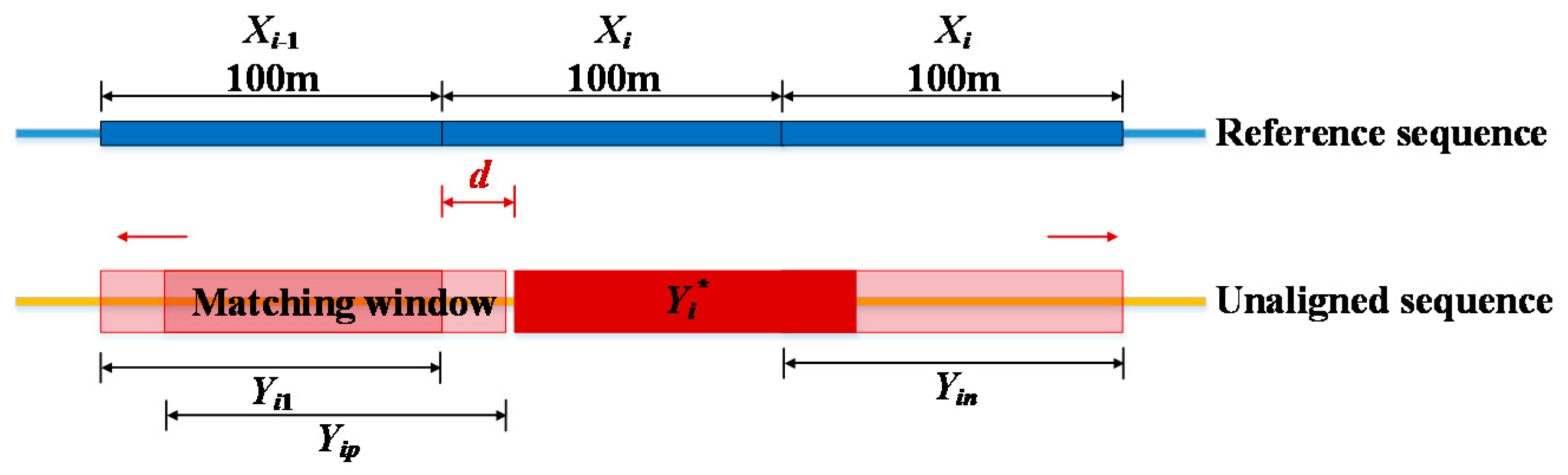
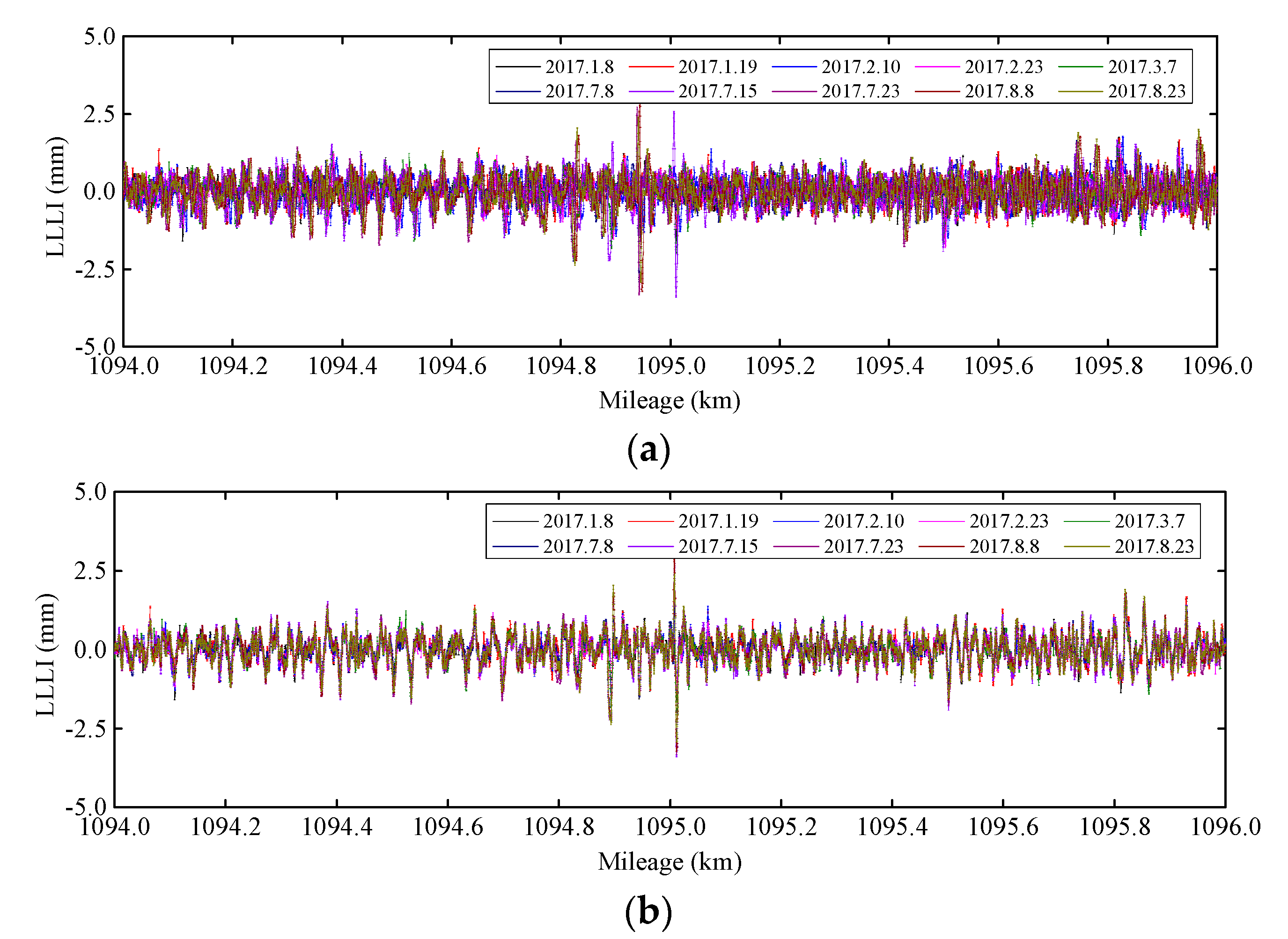
2.2. Data Mile-Point Alignment

Because of the effects of GPS accuracy, uncertain vehicle operating conditions, and complex human interference, there is an absolute error between the measured and actual mile-point values of track inspection data. Field surveys reveal that measured mile-point positions can be off by up to 200 m [49]. Even if the same inspection vehicle is used to detect the same section repeatedly, the mile-point values of each inspection may also be different.

As for slab arching detection, multiple historical data will be compared to determine whether the damages have occurred and developed. Therefore, it is necessary to correct the mile-point error among multiple inspections firstly.

In the normal service without major maintenance, the track geometry data among different inspections have similar waveforms. However, the wheels may slip or slide randomly during operation, thereby distorting the data waveforms in space (i.e., the mile-point deviation changes nonlinearly and randomly with the mileage) [50]. On account of this, we establish a mile-point alignment algorithm combining CA and DTW (CA-DTW). The specific process is as follows.

(1) Sequence segmentation

Firstly, an inspection sequence with high quality is selected as the reference sequence, and its absolute mile-point error is corrected according to infrastructure ledger information. Then, the reference sequence is divided into consecutive 100-m segments (X₁, X₂, …) by mileage. Through correlation-based and DTW-based alignment, each unaligned sequence can be matched with the reference sequence segment by segment.

(2) CA-based initial alignment

As shown in Figure 4, the matching window and X_i are of equal length (i.e., 100 m). Within X_i ± 100 m, the window moves point by point on the unaligned sequence, to obtain different segments (Y_i1, …, Y_ip, …, Y_in) corresponding to X_i. The correlation coefficient ρ between X_i and Y_ip can be calculated by Equation (1)

$$\rho (X_i,Y_{ip})=\frac{Cov(X_i,Y_{ip})}{\sqrt{Var[X_i]Var[Y_{ip}]}}$$

(1)

where Cov(•) is the covariance between the sequences; Var[•] is the variance of the sequence. According to the maximum ρ criterion, the initial aligned segment Y_i^* and deviation distance d can be determined. By shifting initial aligned segments, the initial aligned sequence can be obtained.

(3) DTW-based secondary alignment

DTW is a matching method for similar but warping sequences, which is essentially a dynamic programming problem [51]. It can search the optimal alignment relations between sequences efficiently and has been widely used to process series data [52,53]. Considering the spatial distortion of inspection data, the initial aligned segment Y_i^* is locally scaled based on DTW so that the mileage offset can be further corrected. A dynamic program is established, taking the minimum sum of squared differences between Y_i^* and X_i as the goal. The objective function and constraints are as follows.

$$D=\min {\displaystyle \sum _{j=1}^{size(Y_i{}^{*})}{(Y_i{}^{*}(j)-X_i(P(j)))}^2}+\zeta (j)$$

(2)

$$\zeta (j)=\{\begin{array}{cc}\alpha \times (\frac{M_{X_i}(P(j))-M_{X_i}(P(j-1))}{M_{Y^{*}{}_i}(j)-M_{Y^{*}{}_i}(j-1)}-1{)}^2\hfill & j\ne 1,\alpha =3\\ 0\hfill & j=1\end{array}$$

(3)

$$s.t.\{\begin{array}{l}P(1)=1\\ P(size(Y_{{}_i}^{*}))=size(X_i)\\ -k+j\le P(j)\le k+j\le size(Y_{{}_i}^{*})\\ P(j-1)\le P(j)\end{array}$$

(4)

where j is the point of Y_i^*, P(j) is the point of X_i that matches j, and size(•) is the sample size of the segment. ζ(j) denotes the distance loss, and M_A(•) denotes the mileage coordinates of the point on sequence A. The farther the mileage between P(j-1) and P(j), the higher the distance loss. k is the farthest distance between j and P(j) under consideration. Due to the initial alignment, the remaining deviation is small. After trial calculation, k is set to 4.

Taking the left longitudinal level irregularity (LLLI) of 8 January 2017 as the reference sequence, the CA-DTW method is performed on the inspections of low-temperature and high-temperature months, as shown in Figure 5. It can be seen intuitively that the data mileage deviations of different inspections are well corrected. To analyze the effect of the algorithm further, we use the sum of absolute deviations per kilometer E and correlation coefficient ρ to quantify the deviations of sequences, as shown in

Table 1. Deviation statistics of sequences compared to the reference sequence.

Inspection Date	Unaligned		Aligned
	E/mm	ρ	E/mm	ρ
19 January	860.41	0.7735	473.28	0.9265
10 February	1936.98	−0.1641	515.89	0.9131
23 February	1075.79	0.6300	569.94	0.8925
7 March	1199.81	0.5939	572.70	0.8748
8 July	1850.71	0.0192	663.82	0.8380
15 July	1584.62	0.3777	808.91	0.8151
23 July	1978.14	0.0718	985.99	0.7553
8 August	2000.36	0.0576	841.28	0.7838
23 August	1971.47	0.0310	754.74	0.8167

. We can observe that after alignment, E of each inspection is reduced, and ρ is improved, which shows the feasibility of the algorithm. Moreover, comparing the statistics of aligned inspections, we can find that the values of statistics are related to slab arching. There is a larger deviation and a smaller correlation between the sequence with arching and the reference sequence.

2.3. Arching Characteristics

The inspection data of arched and non-arched segments are contrastively analyzed combined with the maintenance information. It can be found that the arching characteristics are mainly reflected in the longitudinal level irregularity (LLI). Figure 6 shows several arching segments of 15 July 2017, taking the data of 8 January 2017 as reference. A is the semi-crest amplitude, δ is the amplitude difference between different months, and λ is the wavelength. We can observe that different arched segments present various waveforms. Although the waveforms of different months in the specific segment are roughly similar, δ in the arched segment increases compared to the non-arched segment. By statistics, in the arched segments, the maximum value of A exceeds 3 mm, and the value of δ is generally greater than 1 mm. Most values of λ are close to the length of the track slab (6.45 m), and the maximum is less than 10 m.

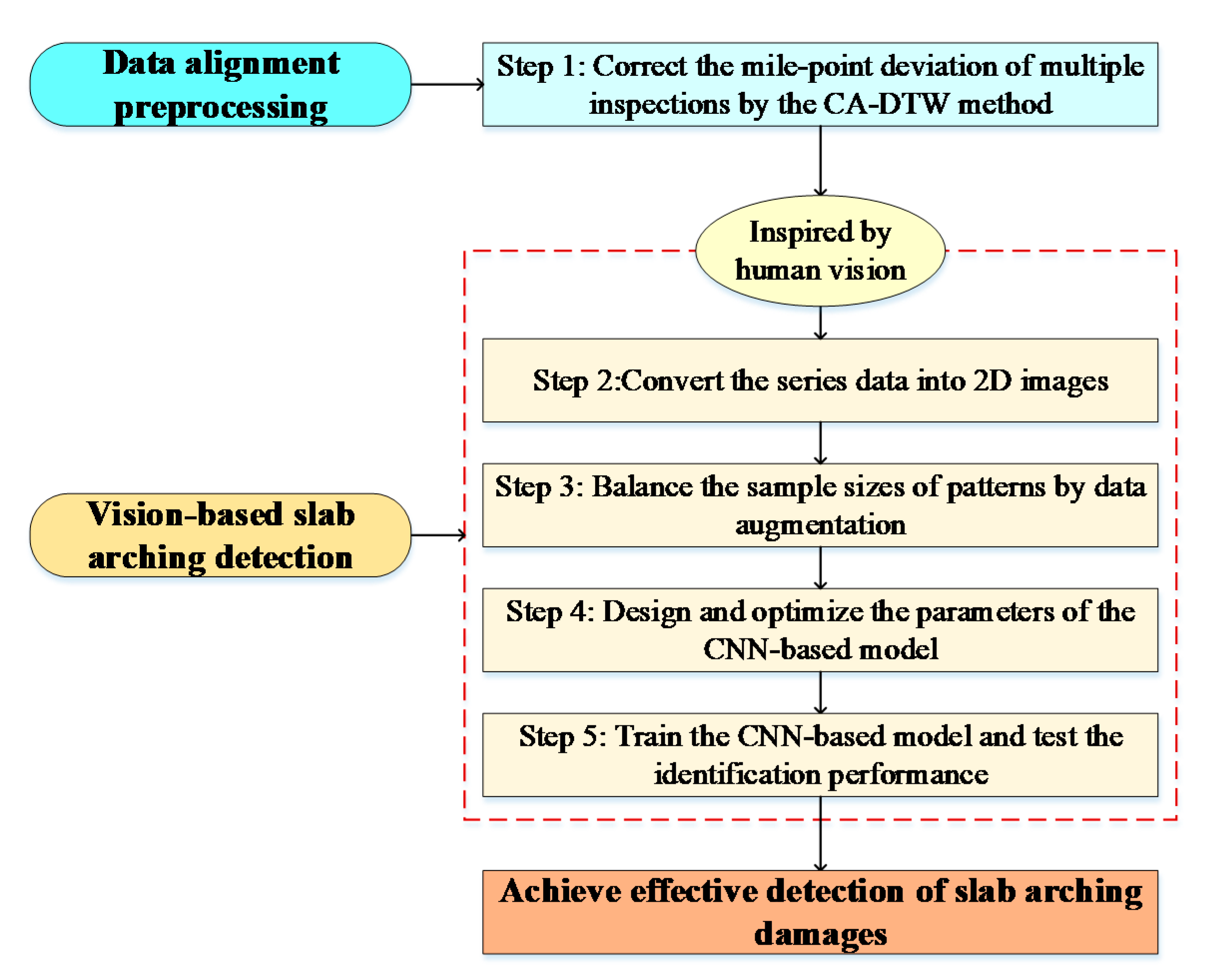
3. Proposed Vision-Based Arching Detection Method

The process of arching detection in this paper includes five steps, as shown in Figure 7. The first step is to preprocess the inspection data by the CA-DTW mile-point alignment method, which is introduced specifically in Section 2.2. Then, inspired by human vision, the original sequences are converted into 2D images (step 2), and the data augmentation is used to balance the number of “Arching” and the number t of “Normal” (step 3). The fourth step is to design the architecture of the CNN-based detection model and optimize the model parameters. The fifth step is to train the detection model repeatedly and test its performance using the established dataset. Through the above steps, the effective arching detection can be achieved. In this section, the details of the dataset establishment and CNN-based detection model are mainly introduced.

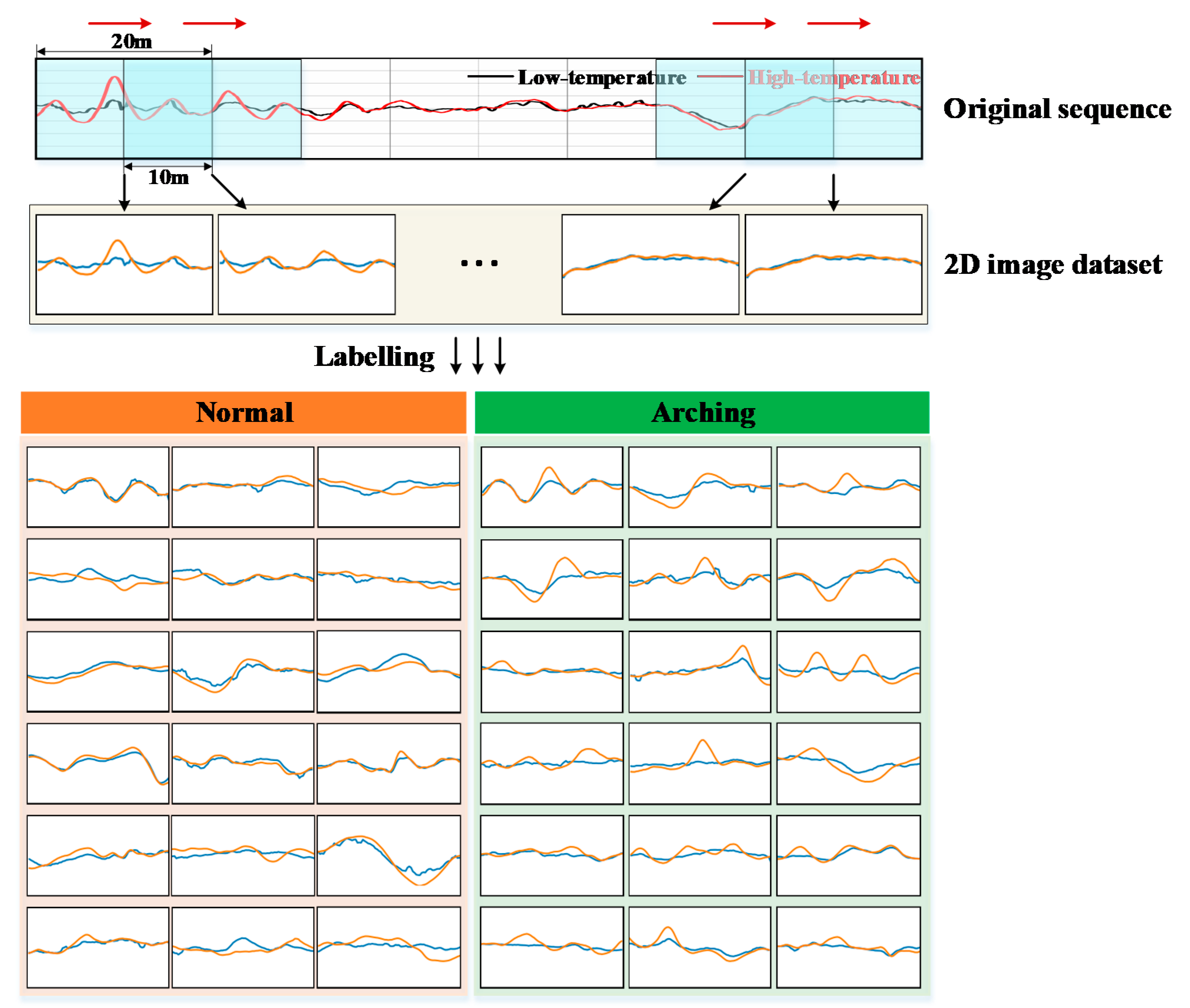
3.1. Data Conversion and Augmentation

In our initial data-based arching detection, a basic technique is to plot and compare the LLI segments of different months manually, and then determine whether the slab arching has occurred or not. To imitate this process, we firstly convert original series data into images, rather than directly inputting the series to the detection model. The arching waveforms in the data have obvious graphical spatial characteristics, which can be more completely preserved in 2D images, thus facilitating clear detection.

The series-image conversion method is displayed in Figure 8. Combining the LLI sequence data of high-temperature month (e.g., July in the northern hemisphere) and low-temperature month (e.g., January in the northern hemisphere), the sliding window is utilized to construct a 2D-image dataset. To ensure the arching characteristics can be fully captured, the window length is set to 20 m, and the overlapping length is 10 m. The size of each image is 250 pixel × 100 pixel, the ordinate range is −4 mm to 4 mm, and the abscissa range is 0 m to 20 m. In the images, the blue line and orange line denote the LLI of the low-temperature month and high-temperature month, respectively. On account of determined axis ranges, the coordinates are invisible because labeled values are not required for the CNN model to learn the arching features. Furthermore, the naming of image files contains arching detection information, including the inspection date, mileage section, and inspection item (LLL/RRL), which is convenient for locating damaged segments.

Following the maintenance information and manual inspection, the images are labeled with “Normal” or “Arching”. We can observe that part of the normal and arching images have some similar characteristics, which can readily be confused.

In actual HSR service, the probability of slab arching is much lower than the normal conditions. The number of arching samples and the number of normal samples are extremely imbalanced, which may cause over-fitting to the normal pattern and under-fitting to the arching pattern. Thus, it is necessary to carry out data augmentation on the arching images to expand the dataset. Common augmentation operations including rotation, flipping, cropping, translation, and scaling. Due to the particularity of the images formed by series data, the arching images are only flipped horizontally to avoid the generation of unnecessary features or the increase of image category, as shown in Figure 9. Moreover, the normal images are randomly downsampled to reduce the normal set. In this way, feature extraction can be better achieved.

3.2. CNN for Slab Arching Detection

CNN is one of the widely utilized deep learning networks proposed by Lecun et al. [54]. It is good at detecting tiny and meaningful spatial features and has the characteristics of sparse weights [55]. In general, CNN is applied to computer vision areas, such as image classification [56] and object detection [57]. Therefore, it is also suitable for the vision-based slab arching detection problem in this paper.

CNN is a stacked architecture employing multiple layers, mainly including convolutional layers, pooling layers, and fully connected layers. The convolutional layer uses a series of kernels to perceive different local features, which can be integrated to form the feature maps expressing global information. Through parameter sharing, the amount of computation can be greatly reduced. The pooling layer is applied to reducing the size of feature maps and ignoring the minute variation by merging local information, thereby filtering out the noise in the original data and preventing over-fitting. After several alternating convolutional-pooling layers, the fully connected layers are used for the final classification based on the extracted features of the previous layers.

Figure 10 shows the final architecture of the CNN detection model. Some parameters of the model are determined through the trial method, and the details are shown in Section 4.1. Firstly, the images are resized to 60 pixel × 60 pixel × 3 channel before inputting to the first convolutional layer. Then, three sets of convolutional-pooling layers are employed for feature extraction. The kernel sizes of convolutional and pooling layers are 5 × 5 and 2 × 2, respectively. The rectified linear units (ReLU) [58] is selected as the activate function following the convolution layer, thus performing a nonlinear transformation on the data space. Moreover, max pooling is adopted in the pooling layers. From the first convolutional layer to the last pooling layer, the sizes of the feature maps are reduced from 56 × 56 to 4 × 4.

Next, the feature maps of the last pooling layer are flattened as a 1D vector and fed into the fully connected layers. The softmax classifier is utilized to compute the predicted probability of each pattern and obtain the final output, as shown in Equation (5).

$$S_k^n=P(\mathrm{prediction}=k|X_n)=\frac{\exp (V_k^n)}{{\displaystyle {\sum }_{k=1}^K\exp (V_k^n)}}$$

(5)

where $S_k^n$ is the kth component for the output vector of sample X_n; P(prediction = k|X_n) represents the predicted probability that sample X_n belongs to pattern k. $V_k^n$ denotes the kth component for the feature vector of sample X_n before softmax processing. K is the number of patterns (i.e., the number of components for the output vector).

During the training process, the “dropout” method is utilized to reduce overfitting in the fully connected layers, and the dropout rate is set to 0.5. Adam optimizer and exponential decay learning rate are chosen to train the model. The initial learning rate is set to 0.001, and the decay rate is 0.95. The loss function is the sum of cross-entropy loss and L₂ regularization loss, which is expressed as follows.

$$Loss=-\frac{1}{N}[{\displaystyle {\sum }_{n=1}^N{\displaystyle {\sum }_{k=1}^K{y}_k^n\log (S_k^n)}}]+\alpha ||w|{|}_2^2$$

(6)

where Loss represents the loss function, and N represents the number of samples in a batch (the batch size is 32).$y_k^n$ is the kth component for the label of sample X_n. w represents the collection of model parameters considering regularization. α is the regularization rate, which is set to 0.001.

4. Results and Discussion

This paper uses the track geometry data from 2016 to 2018 to train and test the proposed detection framework. The inspections of low-temperature months (January to March) and high-temperature months (July to August) of each year are combined in pairs to construct an image dataset. Each inspection contains 315 km of track geometry data, which is much longer than the arching wavelength (less than 10 m). The inspection line passes through different substructures and external environment, so the samples cover waveform characteristics of various conditions. Moreover, the combinations of different inspections can include different degrees of arching from the initial stage to the later stage. Therefore, the dataset contains sufficient features and can meet the need for model training and verification.

According to the data conversion and augmentation method in Section 3.1, the dataset is constructed including 11896 arching images. On this basis, five subsets are used for the research, as shown in

Table 2. Five subsets established for training and testing.

Subset.	Training and Validation Set (Arching: Normal)	Testing Set	Total
1	8922 (2974:5948 = 1:2)	Arching:5948 Normal:5948	20818
2	11896 (5948:5948 = 1:1)		23792
3	11896 (2974:8922 = 1:3)		23792
4	11896 (1700: 10196 = 1:6)		23792
5	23792 (5948:17844 = 1:3)		35688

. As for the training and validation sets, each subset has a different pattern ratio and sample scale, and the proportion of training and validation is 5:1. Subset 2 is a balanced set that provides an equivalent proportion for each type, whereas other subsets are imbalanced sets for comparison studies. Compared with Subset 2, all arching samples used for training and validation in Subset 1 are original images without augmentation operation. Subset 3 and Subset 4 have the same sample size as Subset 2 in training and validation set, but the ratio of “Arching” to “Normal” is 1:3 and 1:6, respectively. The total number of training and validation samples for Subset 5 is twice that of Subset 3, whereas the pattern ratio is the same. Besides, different subsets share the same testing set containing 11896 images, in which the samples in training and validation sets are filtered out.

The model is implemented on the python Tensorflow (1.10.1) deep learning framework. Three error metrics, including Precision, Recall, and F₁-score, are mainly employed to optimize the model structure and assess the model performance. They are defined as follows.

$$\mathrm{Pr}\mathrm{ecision}=\mathrm{TP}/(\mathrm{TP}+\mathrm{FP})\times 100\%$$

(7)

$$\mathrm{Rerall}=\mathrm{TP}/(\mathrm{TP}+\mathrm{FN})\times 100\%$$

(8)

$${\mathrm{F}}_1-\mathrm{score}=2\times \mathrm{Precision}\times \mathrm{Recall}/(\mathrm{Precision}+\mathrm{Recall})$$

(9)

where TP (i.e., True Positive) represents the number of the arching samples that are correctly detected as “Arching”; FP (i.e., False Positive) represents the number of the normal samples that are incorrectly detected as “Arching”; FN (i.e., False Negative) represents the number of the arching samples that are incorrectly detected as “Normal”. Precision reflects the proportion of the actual arching samples in detected “Arching” samples. Recall reflects the proportion of the correctly detected samples in actual arching samples. F₁-score is the harmonic mean of Precision and Recall, which indicates the overall accuracy of the arching detection model.

4.1. CNN Architecture Optimization

There are many hyperparameters in the CNN framework, including the number of convolutional-pooling layers, convolutional kernel size, and the number of fully connected layers. To improve the model performance, we use the balanced set (Subset 2) to adjust and optimal the CNN architecture. According to the control variable method, eight cases are set for trial calculation. Each case is conducted in five runs taking the detection ability on the validation set as the criterion. The mean values of evaluation metrics are tabulated in

Table 3. Arching detection performance of different CNN architectures.

Case	Architecture	Evaluation Metrics (%)			Time/Epoch (s)
		Precision	Recall	F1-Score
1	5 × 5 @ 6, FC 128	94.5	96.6	95.5	13.5
2	5 × 5 @ 6, 5 × 5 @ 12, FC 128	96.5	97.6	97.0	13.8
3	3 × 3 @ 6, 3 × 3 @ 12, 3 × 3 @ 24, FC 128	97.0	97.7	97.3	7.2
4	5 × 5 @ 6, 5 × 5 @ 12, 5 × 5 @ 24, FC 128	97.8	98.2	98.0	14.0
5	7 × 7 @ 6, 7 × 7 @ 12, 7 × 7 @ 24, FC 128	96.7	97.0	96.8	22.6
6	5 × 5 @ 6, 5 × 5 @ 12, 5 × 5 @ 24, FC 128-FC 32	96.8	98.0	97.4	14.4
7	5 × 5 @ 6, 5 × 5 @ 12, 5 × 5 @ 24, FC 512-FC 128	97.9	96.8	97.4	14.6
8	5 × 5 @ 6, 5 × 5 @ 12, 5 × 5 @ 24, FC 512-FC 128-FC 32	95.0	97.7	96.2	14.7

. In the table, Time/Epoch denotes the training time required for each epoch. The convolution layer parameters are represented as “kernel size @ the number of kernels”; the fully connected layer parameters are represented as “FC number of hidden nodes in the layer”.

We can observe that with the increase of convolution-pooling layers (Case 1, 2, and 4), the values of metrics improve. In contrast, the Time/Epoch only slightly changes. The model performance with different convolutional kernel sizes (Case 3, 4, and 5) are also compared. It can be seen that as the kernel size increases, the error metrics first increases and then decreases, whereas the Time/Epoch grows obviously. Furthermore, different fully connected combinations are applied to the model (Case 4, 6, 7, and 8). One fully connected layer with 128 nodes has the highest efficiency.

Comprehensively considering the detection accuracy and calculation time, we choose the architecture of Case 4, whose F₁-score is 98.0%. In the model, the number of convolution-pooling layers is three, the convolutional kernel size is 5 × 5, and the number of kernels is 6, 12, and 24. Moreover, one fully connected layer with 128 nodes is adopted.

4.2. Performance Evaluation with Various Datasets

Besides the optimization of the model architecture, constructing an excellent dataset is also a key to improving the model performance. Accordingly, based on the determined detection framework, the model runs on each subset in Table 2 for five times, and the error metrics are analyzed to evaluate the model performance. The quantity and proportion of each pattern in the testing result (one of five runs) are shown in

Table 4. Quantity and proportion of each pattern in the testing result (one of five runs).

Subset	Arching		Normal		Ground Truth
	Detection Result	Ratio (%)	Detection Result	Ratio (%)
1	5434	45.7	6320	54.3	Arching: 5948 (50%) Normal: 5948 (50%)
2	5924	49.8	5972	50.2
3	5757	48.4	6139	51.6
4	5526	46.4	6370	53.6
5	5785	48.6	6111	51.4

. We can find that the proportions of arching and normal of the detection results are as high as 49.8% and 50.2% (Subset 2), which is quite close to the ground truth. Compared with Subset 2, the detection results of imbalanced sets are more different from the ground truth, especially for Subset 1.

To quantify the detection ability of the proposed method, the error metrics of each subset are calculated as depicted in Figure 11. Regardless of the validation set or the testing set, the F₁-score of each pattern can exceed 98%, showing the high detection accuracy of the proposed model. Specifically, the Precision, Recall, and F₁-score of “Arching” on the testing set (Figure 11b) can reach 98.3%, 98.4%, and 98.4%, respectively.

For the detection of the pattern “Arching”, the cases using Subset 2 outperform the cases using other datasets, as shown in Figure 11a,b. Compared with the metrics of Subset 1, the metrics of Subset 2 are significantly improved, in which the Recall on the testing set increases by 6.2%. It demonstrates that data augmentation operation can effectively enhance the arching feature extraction, thereby improving the model fitting to the pattern “Arching”.

In terms of the data imbalance impact on model performance, Subset 2, Subset 3, Subset 4, and Subset 5 are used for comparative research. At the same training size, with the imbalance degree (i.e., the ratio of “Normal” to “Arching”) increases, the overall detection performance of both the validation set and testing set decreases. As the pattern ratio changes from 1:1 to 6:1, the F₁-score of the validation set decreases from 98.0% to 92.5%, and the F₁-score of the testing set decreases from 98.4% to 96.3%. It is mainly because the reduction of arching training samples leads to the insufficient learning of arching features. At the same pattern ratio, with the increase of training size, the performance of the imbalanced set improves. However, its performance is still not as good as the balanced set, and the increase in training size means that more time is required for model training.

For the detection of the pattern “Normal”, since there are more normal samples in the imbalanced sets, the performance on the validation set is slightly improved from the balanced set to the imbalanced sets. Nevertheless, the performance on the testing set decreases to some extent, which may be due to the different pattern ratio of the validation and testing set, as shown in

Table 5. Detection results of the validation set and testing set (one of five runs).

Subset	Validation Set				Testing Set
	TP	TN	FP	FN	TP	TN	FP	FN
1	473	977	15	23	5349	5863	85	599
2	962	970	22	30	5823	5847	101	125
3	477	1472	16	19	5693	5884	64	255
4	262	1680	20	22	5467	5889	59	481
5	956	2948	26	36	5741	5904	44	207

. In the imbalanced set, the number of arching samples of the validation set is far less than that of the testing set. Therefore, despite the high proportion of TN (i.e., True Negative, represents the number of the normal samples that are correctly detected as “Normal”) in the testing result, the FN increases sharply compared to the validation result, and its influence is non-negligible. Thus, the testing results and validation results of “Normal” present different rules.

Overall, the balanced set (Subset 2) has the best performance and can achieve accurate detection for both “Arching” and “Normal patterns. Therefore, in practice, we should construct balanced datasets to detect slab arching.

4.3. Comparison Study with DNN

To verify the superiority of the proposed framework, we adopt the plain DNN for comparison study. DNN is a typical deep learning network and has been employed in data anomaly detection with high accuracy [59]. During the training process, the model parameters of the DNN are firstly adjusted to ensure the best performance. Then, five subsets are adopted to train and test the model. In this part, we use F₁-score on the testing set and Time/Epoch as indicators to compare the performance of the proposed model and the DNN, as shown in Figure 12.

It can be observed that whether training with balanced or imbalanced sets, the proposed CNN-based method has higher detection accuracy and shorter training time compared with the DNN model. To quantitatively analyze the superiority of the proposed model, a performance improvement index (PDI) is established as follows.

$$PDI=\left|I_{proposed}-I_{DNN}\right|/I_{DNN}$$

(10)

where I_proposed and I_DNN represent the evaluation indicators of the proposed model and DNN model, respectively.

According to Equation (10), the improvements in accuracy and cost of the proposed model are calculated in

Table 6. Performance improvement of the proposed model compared with the DNN model.

PDI	Subset 1	Subset 2	Subset 3	Subset 4	Subset 5
F1-score	1.5	0.7	1.5	3.4	1.5
Time/Epoch	0.6	0.6	0.6	0.6	0.6

. Compared with the DNN model, the F₁-score of the proposed model increases up to 3.4 times, and the training time is reduced by 0.6. It reflects the powerful spatial feature extraction capability of CNN. By contrast, the performance of the DNN model is poor. It can hardly detect slab arching, especially for the cases of using imbalanced sets. It is because the arching features included in track irregularities are very tiny and similar to normal waveforms. However, DNN changes the original positional relations between pixels by transforming the two-dimensional matrix (image) into a one-dimensional vector, which may make it difficult to learn sufficient characteristics. Moreover, all results of the balanced set are better than that of the imbalanced sets, again proving the advantages of the balanced training set.

4.4. Detection Result Analysis

To further study the detection results of the proposed model, we analyze the examples of detected and undetected arching in the testing result. As shown in Figure 13a, the proposed model can detect arching images with different shapes and degrees and avoid the influence of data noise. However, DNN cannot detect these samples due to its poor learning ability of graphical features.

Some examples of undetected arching are shown in Figure 13b. Among 5948 arching images of the testing set, 125 arching images are not detected, accounting for 2.1% of the total. The error is within an acceptable range and can be further corrected through on-site rechecking. Through analyzing the cause of the error, we can find that it is difficult to detect the arching in the early stage accurately. In the early stage, the arching features reflected on the LLI data are tiny because of the small deformation of the track slabs. Therefore, these samples have high similarity with normal samples, which increases the detection difficulty.

5. Conclusions

In this paper, a novel framework is proposed for slab arching detection using track geometry data. Based on human vision simulation, the method converts the original series data into 2D images and utilizes CNN for feature extraction and arching detection. The main conclusions are as follows.

(1)

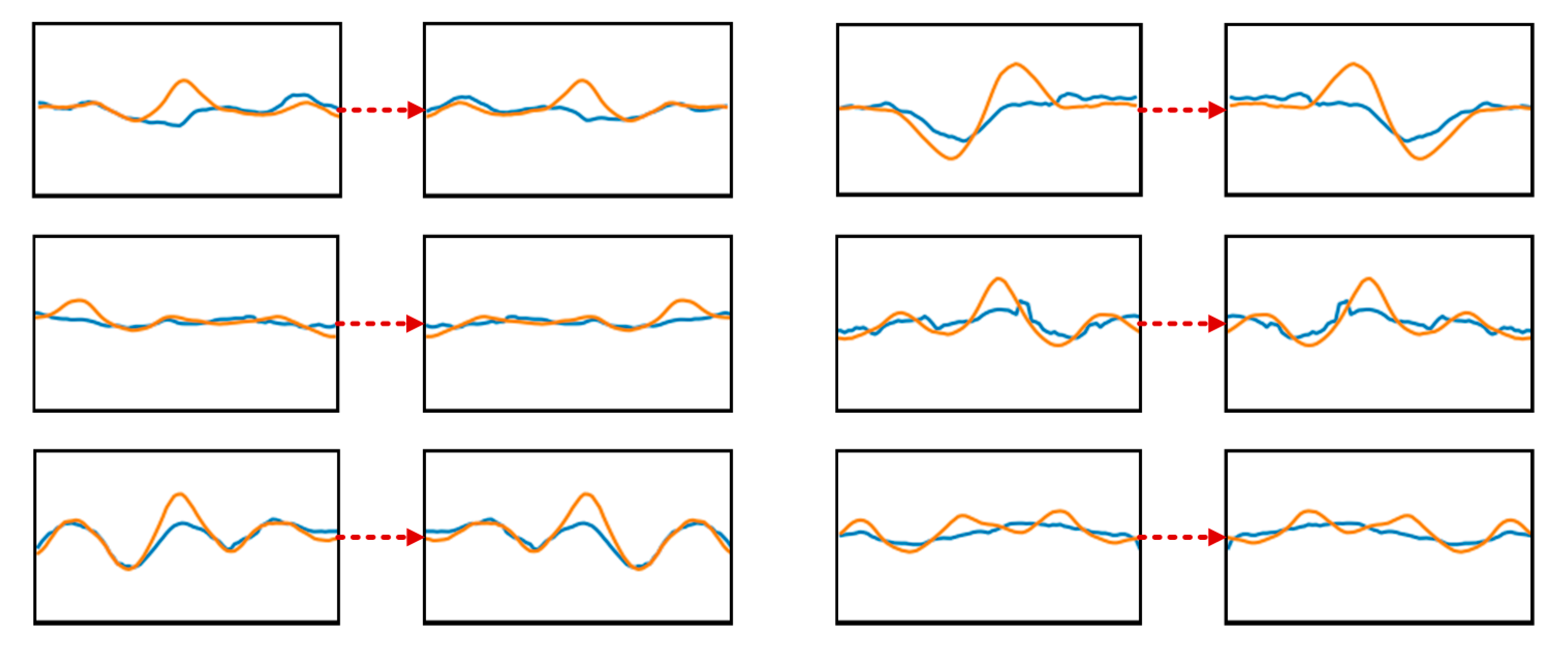
The alignment algorithm combining correlation analysis and DTW can correct the milepost deviation of different inspections effectively. Based on the aligned data, it is found that the longitudinal level irregularities can reflect slab arching, and the data wavelengths are close to the length of the track slab.

(2)

The proposed detection framework can accurately detect arching damage, whose Precision, Recall, and F₁-score can reach 98.3%, 98.4%, and 98.4%, respectively. Moreover, the data augmentation operation and balanced set establishment can help the model extract arching features more adequately and improve the performance. As the pattern ratio changes from 6:1 to 1:1, the F₁-score can increase from 92.5% to 98.0%.

(3)

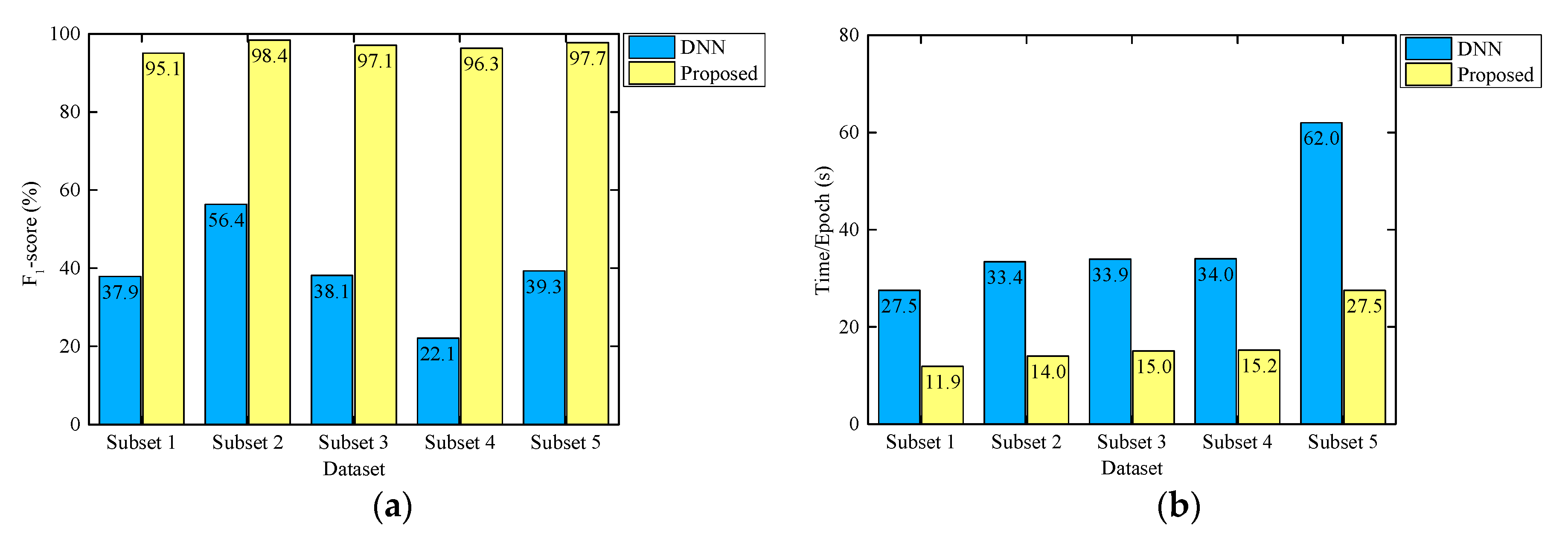
The proposed framework outperforms the plain DNN model, showing the excellent spatial characteristics learning ability. Compared to the plain DNN, the F₁-score of the proposed model increases up to 3.4 times, and the training time is reduced by 0.6.

In practice, engineers can use the proposed vision-based method to accurately detect slab arching, quickly locate the damage sections, and promote the achievement of intelligent maintenance decisions. Additionally, the method can be expanded to other damage detection of track structures based on series data.

References

1. Gao, L.; An, B.; Xin, T.; Wang, J.; Wang, P. Measurement, analysis, and model updating based on the modal parameters of high-speed railway ballastless track. Measurement 2020, 161, 107891. [Google Scholar] [CrossRef]
2. Ando, K.; Sunaga, M.; Aoki, H.; Haga, O. Development of slab tracks for Hokuriku Shinkansen line. Q. Rep. RTRI 2001, 42, 35–41. [Google Scholar] [CrossRef]
3. Li, T.; Su, Q.; Shao, K.; Liu, J. Numerical analysis of vibration responses in high-speed railways considering mud pumping defect. Shock Vib. 2019, 2019, 9707909. [Google Scholar] [CrossRef] [Green Version]
4. Zhong, Y.; Gao, L.; Zhang, Y. Effect of daily changing temperature on the curling behavior and interface stress of slab track in construction stage. Constr. Build. Mater. 2018, 185, 638–647. [Google Scholar] [CrossRef]
5. Zhao, L.; Zhou, L.-Y.; Zhang, G.-C.; Wei, T.-Y.; Mahunon, D.A.; Jiang, L.-Q.; Zhang, Y.-Y. Experimental study of the temperature distribution in CRTS-II ballastless tracks on a high-speed railway bridge. Appl. Sci. 2020, 10, 1980. [Google Scholar] [CrossRef] [Green Version]
6. Zhu, S.; Wang, M.; Zhai, W.; Cai, C.; Zhao, C.; Zeng, D.; Zhang, J. Mechanical property and damage evolution of concrete interface of ballastless track in high-speed railway: Experiment and simulation. Constr. Build. Mater. 2018, 187, 460–473. [Google Scholar] [CrossRef]
7. Xu, Y.; Yan, D.; Zhu, W.; Zhou, Y. Study on the mechanical performance and interface damage of CRTS II slab track with debonding repairment. Constr. Build. Mater. 2020, 257, 119600. [Google Scholar] [CrossRef]
8. Yu, Z.; Xie, Y.; Shan, Z.; Li, X. Fatigue performance of CRTS III slab ballastless track structure under high-speed train load based on concrete fatigue damage constitutive law. J. Adv. Concr. Technol. 2018, 16, 233–249. [Google Scholar] [CrossRef] [Green Version]
9. Zhu, S.; Fu, Q.; Cai, C.; Spanos, P.D. Damage evolution and dynamic response of cement asphalt mortar layer of slab track under vehicle dynamic load. Sci. China Technol. Sci. 2014, 57, 1883–1894. [Google Scholar] [CrossRef]
10. Ren, J.; Wang, J.; Li, X.; Wei, K.; Li, H.; Deng, S. Influence of cement asphalt mortar debonding on the damage distribution and mechanical responses of CRTS I prefabricated slab. Constr. Build. Mater. 2020, 230, 116995. [Google Scholar] [CrossRef]
11. Peng, H.; Zhang, Y.; Wang, J.; Liu, Y.; Gao, L. Interfacial bonding strength between cement asphalt mortar and concrete in slab track. J. Mater. Civ. Eng. 2019, 31, 04019107. [Google Scholar] [CrossRef]
12. Wang, J.; Zhou, Y.; Wu, T.; Wu, X. Performance of cement asphalt mortar in ballastless slab track over high-speed railway under extreme climate conditions. Int. J. Geomech. 2019, 19, 04019037. [Google Scholar] [CrossRef]
13. Ren, J.; Li, X.; Yang, R.; Wang, P.; Xie, P. Criteria for repairing damages of CA mortar for prefabricated framework-type slab track. Constr. Build. Mater. 2016, 110, 300–311. [Google Scholar] [CrossRef]
14. Li, Y.; Chen, J.; Wang, J.; Shi, X.; Chen, L. Analysis of damage of joints in CRTSII slab track under temperature and vehicle Loads. KSCE J. Civ. Eng. 2020, 24, 1209–1218. [Google Scholar] [CrossRef]
15. Liu, X.; Zhang, W.; Xiao, J.; Liu, X.; Li, W. Damage mechanism of broad-narrow Joint of CRTSII slab track under temperature rise. KSCE J. Civ. Eng. 2019, 23, 2126–2135. [Google Scholar] [CrossRef]
16. Cai, X.-P.; Luo, B.-C.; Zhong, Y.-L.; Zhang, Y.-R.; Hou, B.-W. Arching mechanism of the slab joints in CRTSII slab track under high temperature conditions. Eng. Fail. Anal. 2019, 98, 95–108. [Google Scholar] [CrossRef]
17. Yang, R.; Li, J.; Kang, W.; Liu, X.; Cao, S. Temperature characteristics analysis of the ballastless track under continuous hot weather. J. Transp. Eng. A-Syst. 2017, 143, 04017048. [Google Scholar] [CrossRef]
18. Ren, J.; Deng, S.; Jin, Z.; Yang, J.; Liu, X. Energy method solution for the vertical deformation of longitudinally coupled prefabricated slab track. Math. Probl. Eng. 2017, 2017, 8513240. [Google Scholar] [CrossRef] [Green Version]
19. Li, Z.-W.; Liu, X.-Z.; He, Y.-L. Identification of temperature-induced deformation for HSR slab track using track geometry measurement data. Sensors 2019, 19, 5446. [Google Scholar] [CrossRef] [Green Version]
20. Song, X.; Zhao, C.; Zhu, X. Temperature-induced deformation of CRTS II slab track and its effect on track dynamical properties. Sci. China Technol. Sci. 2014, 57, 1917–1924. [Google Scholar] [CrossRef]
21. Resendiz, E.; Hart, J.M.; Ahuja, N. Ahuja Automated visual inspection of railroad tracks. IEEE Trans. Intell. Transp. 2013, 14, 751–760. [Google Scholar] [CrossRef] [Green Version]
22. Shao, P.; Li, H.; Wu, S.; Wang, T.; Liu, Z.; Li, H. Measurement and research on temperature warping of CRTSI track slab and crack between track slab and cement asphalt motar cushion. China Railway Sci. 2013, 34, 18–22. [Google Scholar] [CrossRef]
23. Xu, J.; Wang, P.; An, B.; Ma, X.; Chen, R. Damage detection of ballastless railway tracks by the impact-echo method. Proc. Int. Civil Eng. Transp. 2018, 171, 106–114. [Google Scholar] [CrossRef]
24. Zhang, J.-K.; Yan, W.; Cui, D.-M. Concrete condition assessment using impact-echo method and extreme learning machines. Sensors 2016, 16, 447. [Google Scholar] [CrossRef] [PubMed]
25. Yang, Y.; Zhao, W.; Du, Y.; Zhang, H. Analysis on directional feature extraction for the target identification of shallow subsurface based on curvelet transform. DYNA 2017, 92, 293–299. [Google Scholar] [CrossRef] [Green Version]
26. Huang, J.; Su, Q.; Liu, T.; Wang, W. Behavior and control of the ballastless track-subgrade vibration induced by high-speed trains moving on the subgrade bed with mud pumping. Shock Vib. 2019, 2019, 9838952. [Google Scholar] [CrossRef]
27. Xu, J.; Ping, W.; Hao, L.; Hu, Z.; Rong, C. Identification of internal damage in ballastless tracks based on Gaussian curvature mode shapes. J. Vibroeng. 2016, 18, 5217–5229. [Google Scholar] [CrossRef] [Green Version]
28. Tang, Y. Displacement monitoring using distributed macro-strain measurement. In Proceedings of the 4th International Conference on Sensors, Measurement and Intelligent Materials (ICSMIM), Shenzhen, China, 27–28 December 2015; Atlantis Press: Paris, France, 2016; Volume 43, pp. 1103–1106. [Google Scholar]
29. Minardo, A.; Coscetta, A.; Porcaro, G.; Giannetta, D.; Bernini, R.; Zeni, L. Distributed optical fiber sensors for integrated monitoring of railway infrastructures. In Proceedings of the 23rd International Conference on Optical Fibre Sensors, Santander, Spain, 2–6 June 2014; Volume 9157. [Google Scholar]
30. Lestoille, N.; Soize, C.; Funfschilling, C. Stochastic prediction of high-speed train dynamics to long-term evolution of track irregularities. Mech. Res. Commun. 2016, 75, 29–39. [Google Scholar] [CrossRef] [Green Version]
31. Mohammadi, R.; He, Q.; Ghofrani, F.; Pathak, A.; Aref, A. Exploring the impact of foot-by-foot track geometry on the occurrence of rail defects. Transport. Res. C Emer. 2019, 102, 153–172. [Google Scholar] [CrossRef]
32. Sharma, S.; Cui, Y.; He, Q.; Mohammadi, R.; Li, Z. Data-driven optimization of railway maintenance for track geometry. Transport. Res. C Emer. 2018, 90, 34–58. [Google Scholar] [CrossRef]
33. Li, C.; Wang, P.; Gao, T.; Wang, J.; Yang, C.; Liu, H.; He, Q. Spatial–temporal model to identify the deformation of underlying high-speed railway infrastructure. J. Transp. Eng. A Syst. 2020, 146, 04020084. [Google Scholar] [CrossRef]
34. Neuhold, J.; Vidovic, I.; Marschnig, S. Preparing track geometry data for automated maintenance planning. J. Transp. Eng. A Syst. 2020, 146, 04020032. [Google Scholar] [CrossRef]
35. Xin, T.; Famurewa, S.M.; Gao, L.; Kumar, U.; Zhang, Q. Grey-system-theory-based model for the prediction of track geometry quality. P. I. Mech. Eng. F J. Rai. 2015, 230, 1735–1744. [Google Scholar] [CrossRef]
36. Andrade, A.R.; Teixeira, P.F. Statistical modelling of railway track geometry degradation using Hierarchical Bayesian models. Reliab. Eng. Syst. Saf. 2015, 142, 169–183. [Google Scholar] [CrossRef] [Green Version]
37. Yang, Y.; Liu, G.; Wang, X. Time–frequency characteristic analysis method for track geometry irregularities based on multivariate empirical mode decomposition and Hilbert spectral analysis. Veh. Syst. Dyn. 2020, 1–24. [Google Scholar] [CrossRef]
38. Guler, H. Prediction of railway track geometry deterioration using artificial neural networks: A case study for Turkish state railways. Struct. Infrastruct. Eng. 2014, 10, 614–626. [Google Scholar] [CrossRef]
39. Ma, L.; Xie, W.; Zhang, Y. Blister defect detection based on convolutional neural network for polymer lithium-ion battery. Appl. Sci. 2019, 9, 85. [Google Scholar] [CrossRef] [Green Version]
40. Zhou, T.; Wang, Y.; Wang, C.; Salous, S.; Liu, L.; Tao, C. Multi-feature fusion based recognition and relevance analysis of propagation scenes for high-speed railway channels. IEEE T. Veh. Technol. 2020, 69, 8107–8118. [Google Scholar] [CrossRef]
41. Wang, Q.; Bu, S.; He, Z. Achieving predictive and proactive maintenance for high-speed railway power equipment with LSTM-RNN. IEEE T. Ind. Inform. 2020, 16, 6509–6517. [Google Scholar] [CrossRef]
42. Han, Y.; Liu, Z.; Lyu, Y.; Liu, K.; Li, C.; Zhang, W. Deep learning-based visual ensemble method for high-speed railway catenary clevis fracture detection. Neurocomputing 2020, 396, 556–568. [Google Scholar] [CrossRef]
43. Lyu, Y.; Han, Z.; Zhong, J.; Li, C.; Liu, Z. A Generic Anomaly Detection of Catenary Support Components Based on Generative Adversarial Networks. IEEE T. Instrum Meas. 2020, 69, 2439–2448. [Google Scholar] [CrossRef]
44. Ma, S.; Gao, L.; Liu, X.; Lin, J. Deep learning for track quality evaluation of high-speed railway based on vehicle-body vibration prediction. IEEE Access 2019, 7, 185099–185107. [Google Scholar] [CrossRef]
45. Peng, D.; Liu, Z.; Wang, H.; Qin, Y.; Jia, L. A novel deeper one-dimensional CNN With Residual Learning for fault diagnosis of wheelset bearings in high-speed trains. IEEE Access 2019, 7, 10278–10293. [Google Scholar] [CrossRef]
46. Hamadache, M.; Dutta, S.; Olaby, O.; Ambur, R.; Stewart, E.; Dixon, R. On the fault detection and diagnosis of railway switch and crossing systems: An overview. Appl. Sci. 2019, 9, 5129. [Google Scholar] [CrossRef] [Green Version]
47. Oneto, L.; Fumeo, E.; Clerico, G.; Canepa, R.; Papa, F.; Dambra, C.; Mazzino, N.; Anguita, D. Dynamic delay predictions for large-scale railway networks: Deep and shallow extreme learning machines tuned via thresholdout. IEEE Trans. Syst. Man Cybern. Syst. 2017, 47, 2754–2767. [Google Scholar] [CrossRef]
48. Ye, T.; Zhang, Z.; Zhang, X.; Zhou, F. Autonomous railway traffic object detection using feature-enhanced single-shot detector. IEEE Access 2020, 8, 145182–145193. [Google Scholar] [CrossRef]
49. Xu, P.; Sun, Q.; Liu, R.; Souleyrette, R.R.; Wang, F. Optimizing the alignment of inspection data from track geometry cars. Comput. Aided Civ. Inf. 2015, 30, 19–35. [Google Scholar] [CrossRef]
50. Xu, P.; Sun, Q.-X.; Liu, R.-K.; Wang, F.-T. Key equipment identification model for correcting milepost errors of track geometry data from track inspection cars. Transp. Res. C Emerg. Technol. 2013, 35, 85–103. [Google Scholar] [CrossRef]
51. Myers, C.; Rabiner, L.; Rosenberg, A. Performance tradeoffs in dynamic time warping algorithms for isolated word recognition. IEEE Trans. Acoust. Speech Signal Process. 1980, 28, 623–635. [Google Scholar] [CrossRef]
52. Liu, L.; Li, W.; Jia, H. Method of time series similarity measurement based on dynamic time warping. CMC-Comput. Mater. Contin. 2018, 57, 97–106. [Google Scholar] [CrossRef]
53. Li, H.; Wang, C. Similarity measure based on incremental warping window for time series data mining. IEEE Access 2019, 7, 3909–3917. [Google Scholar] [CrossRef]
54. Pak, U.; Kim, C.; Ryu, U.; Sok, K.; Pak, S. A hybrid model based on convolutional neural networks and long short-term memory for ozone concentration prediction. Air Qual. Atmos. Health 2018, 11, 883–895. [Google Scholar] [CrossRef]
55. Liang, K.; Qin, N.; Huang, D.; Fu, Y. Convolutional Recurrent Neural Network for Fault Diagnosis of High-Speed Train Bogie. Complexity 2018, 2018, 4501952. [Google Scholar] [CrossRef] [Green Version]
56. Prappacher, N.; Bullmann, M.; Bohn, G.; Deinzer, F.; Linke, A. Defect detection on rolling element surface scans using neural image segmentation. Appl. Sci. 2020, 10, 3290. [Google Scholar] [CrossRef]
57. Murthy, B.C.; Hashmi, F.M.; Bokde, D.N.; Geem, W.Z. Investigations of object detection in images/videos using various deep learning techniques and embedded platforms—A comprehensive review. Appl. Sci. 2020, 10, 3280. [Google Scholar] [CrossRef]
58. LeCun, Y.; Bengio, Y.; Hinton, G. Deep learning. Nature 2015, 521, 436–444. [Google Scholar] [CrossRef]
59. Bao, Y.; Tang, Z.; Li, H.; Zhang, Y. Computer vision and deep learning–based data anomaly detection method for structural health monitoring. Struct. Health Monit. 2018, 18, 401–421. [Google Scholar] [CrossRef]
Figure 1. Prefabricated track slab of China Railway Track System II (CRTSII) slab track system.
Applsci 10 06799 g001
Figure 2. Diagram of slab arching.
Applsci 10 06799 g002
Figure 3. Inspection items of the test line. (a) LLL; (b) LA; (c) Gauge; (d) Cross-level; (e) VAC.
Applsci 10 06799 g003
Figure 4. Correlation-based initial alignment algorithm.
Applsci 10 06799 g004
Figure 5. The inspection data before and after alignment. (a) The data before alignment; (b) The data after alignment.
Applsci 10 06799 g005
Figure 6. Several arching segments of 15 July 2017 taking the data 8 January 2017 as reference. (a) The segment between K1086 + 600 and K1086 + 650; (b) The segment between K1094 + 870 and K1094 + 920.
Applsci 10 06799 g006
Figure 7. Flow chart of slab arching detection.
Applsci 10 06799 g007
Figure 8. Series-image conversion method.
Applsci 10 06799 g008
Figure 9. Data augmentation through horizontal flipping.
Applsci 10 06799 g009
Figure 10. Final architecture of the convolutional neural network (CNN) detection model.
Applsci 10 06799 g010
Figure 11. Model performance evaluation using different datasets. (a) Arching detection performance on the validation set; (b) Arching detection performance on the testing set; (c) Normal detection performance on the validation set; (d) Normal detection performance on the testing set.
Applsci 10 06799 g011
Figure 12. Detection performance comparison of the proposed model and the deep neural network (DNN) model. (a) F1-score on the testing set; (b) Time/Epoch.
Applsci 10 06799 g012
Figure 13. Examples of detected and undetected arching images in the testing set using the proposed model. (a) Examples of correctly detected arching images that cannot be detected by DNN; (b) Examples of undetected arching images.
Applsci 10 06799 g013