Training Set Enlargement Using Binary Weighted Interpolation Maps for the Single Sample per Person Problem in Face Recognition

Abstract

We propose a method of enlarging the training dataset for a single-sample-per-person (SSPP) face recognition problem. The appearance of the human face varies greatly, owing to various intrinsic and extrinsic factors. In order to build a face recognition system that can operate robustly in an uncontrolled, real environment, it is necessary for the algorithm to learn various images of the same person. However, owing to limitations in the collection of facial image data, only one sample can typically be obtained, causing difficulties in the performance and usability of the method. This paper proposes a method that analyzes the changes in pixels in face images associated with variations by extracting the binary weighted interpolation map (B-WIM) from neutral and variational images in the auxiliary set. Then, a new variational image for the query image is created by combining the given query (neutral) image and the variational image of the auxiliary set based on the B-WIM. As a result of performing facial recognition comparison experiments on SSPP training data for various facial-image databases, the proposed method shows superior performance compared with other methods.

1. Introduction

Face recognition technology is used to identify individuals from their captured facial images by leveraging a labeled database containing people’s identities. Compared with other types of biometric recognition, face recognition is less invasive and does not require a subject to be in proximity to or in contact with a sensor, making the method widely applicable to user identification, e-commerce, access control, surveillance, and human–computer interaction. However, because variations caused by extrinsic factors (e.g., illumination and pose) and intrinsic factors (e.g., facial expression, age, and accessories) are very large, it is difficult to robustly recognize a face under uncontrolled conditions [1,2]. To deal with these variations, facial recognition methods have been studied under the assumption that several images can be made available for each person, and high-performance methods have been built using vast databases of this nature (e.g., VGGface2 [3], Tufts Face [4], UMDfaces [5]), MegaFace [6], and LFW [7,8] databases).

However, for many large-scale face recognition applications (e.g., passport authentication, drivers’ license identification, and police investigations), the training data required to learn algorithms do not offer many samples per person. In many cases, there is only a single sample per person (SSPP) available [9,10]. For example, law enforcement agencies have constructed databases of facial images (i.e., mug-shots) for decades. The related datasets comprise frontal face images under steady illumination and blank expressions. However, owing to cost and privacy issues, these databases are rarely augmented with extra multi-conditional candid photos. Furthermore, it is known that criminals usually attempt to disguise their identities when committing a crime [11,12]. Even if they do not, it remains very difficult for systems to match active faces with the collected neutral images. As such, the dearth of learnable data restricts the use of feature-extraction and various other supervised methods [13,14,15,16].

To solve the SSPP problem, several methods of enlarging training datasets have been proposed to generate new images from a given one. The theory of the evolution of technology suggests that such datasets can be expanded using existing means [17,18,19,20]. In E${\left(\mathrm{PC}\right)}^2$A2+ [21], extended from ${\left(\mathrm{PC}\right)}^2$A [22], an image and its corresponding half-, first-, and second-order projected images were used as the training set. In the ${\left(2\mathrm{D}\right)}^2$PCA method [23], new images were generated by simultaneously applying two-directional principal component analysis (PCA) [24] in the row and column directions of 2D images. In the SPCA+ method [25], the training set was enlarged by combining the original image linearly with its derived image obtained by perturbing the image matrix’s singular values. In [26], concatenated left- and right-side images obtained from the symmetry of the face were used as training samples. In [27], images were generated using a symmetry transform for the intraclass and a linear combination for the interclass. In the interclass relationship (ICR) [28], data were generated by a weighted combination of (at least) two images in the training set. The ICR rectified the underestimated intraclass and overestimated the interclass. In MVI [29], the training set was enlarged by generating multiple low-resolution virtual images using a single high-resolution image. In SRGES [30], images were generated by adding mean images of the difference between neutral and variational images for each variation in the auxiliary set to the query image. In [31], occluded images were generated by using a weighted interpolation map and an auxiliary set. The weighted interpolation map represented the degrees of changes in pixels at the same positions between an image and its occluded version. The degree of changes was measured using the standard deviation of the difference between neutral and variational images in the auxiliary set. When generating a new image, the pixels at positions of large differences were replaced with the pixel values of the average image of the occluded images in the auxiliary set.

In this paper, we propose binary weighted interpolation maps (B-WIM) to enlarge the training set for face recognition. Generally, the occurrence of variations leads the local pixels to change in the face image. Supposing it is possible to grasp the change in local pixels between the original and varied images, it then becomes possible to capture the characteristics of the image changes caused by the variation. By analyzing these characteristics, the proposed method can maintain most of the characteristics of the neutral image while replacing only the changed areas with the pixel values of the variational one. For this, we first construct an auxiliary set consisting of neutral images and their variational images. Then, the normalized weighted interpolation map is extracted by using the log-scaled standard deviation of the absolute difference between the neutral images and the corresponding variational images in the auxiliary set. Each element of the weighted interpolation map reflects the degree of change caused by the variation in individual pixels, and a B-WIM is obtained via binarization.

When generating a new image for a given query (neutral) image, the variational image corresponding to the neutral image having the highest correlation with the query image is selected from the auxiliary set. Then, a new image is generated by combining the query and selected variational images. The overall procedure of the proposed method is shown in Figure 1.

The idea for the proposed method was motivated by the ICR concept and the weighted interpolation map method, which are face-generating frameworks. However, unlike ICR, by simply increasing the number of images by the weight combinations of two images, the proposed method has the advantage of generating a natural image with a specific variation. Additionally, the proposed method creates an image of higher quality than the weighted interpolation map (WIM) method by selecting the neutral image and the variational image corresponding to the query image.

Face recognition experiments are evaluated using the following criteria. First, we measure the change in the face recognition rate according to the degree of variation of different databases. Second, the face recognition performance is analyzed using unsupervised and supervised learning methods. Finally, the overall face recognition rates of all methods are assessed. We compare the proposed method with other methods dealing with the SSPP problem: WIM, ICR, E(${\mathrm{PC}}^2$)A+, SPCA+, ${\left(2\mathrm{D}\right)}^2$PCA, SLC, MVI, and SRGES. The results of the experiment show that the proposed method exhibits high face recognition performance for all criteria.

The remainder of this paper is organized as follows. Section 2 explains the proposed method for generating data and describes each procedure in detail. The experimental face recognition results are described in Section 3, and the discussion and conclusion follow.

2. Proposed Method

Using ICR [28], a new image, ${\mathbf{I}}_{new}$, is generated using a weighted combination of neutral images, ${\mathbf{I}}_i$ and ${\mathbf{I}}_j$, as

$${\mathbf{I}}_{new}=(1-\lambda )·{\mathbf{I}}_i+\lambda ·{\mathbf{I}}_j,\mathrm{where}0\le \lambda \le 1$$

(1)

In Equation (1), the weight, $\lambda$, decides the ratio of ${\mathbf{I}}_i$ and ${\mathbf{I}}_j$ to be reflected in ${\mathbf{I}}_{new}$. If $\lambda$ is $0.5$, the two images are assumed to have been reflected equally. In the case of ICR, it is easy to generate images by applying a single parameter for all pixels. However, the changes in some areas within the image will not be reflected accurately, owing to variations. Extrinsic factors, such as occlusions, cause changes in the neutral image. For example, pixels around the eyes change significantly when wearing sunglasses. On the other hand, areas unrelated to these variations generally retain the pixel information of the neutral image. Therefore, it is necessary to obtain the weights for each pixel.

In this paper, we propose a method to enlarge the training set. A new image, ${\mathbf{I}}_{new}$, with variations, is generated via a combination of the neutral image, $\mathbf{I}$, and the variational image, $\widehat{\mathbf{I}}$, derived from $\mathbf{I}$ by referring to the ICR. The method of generating a new image is redefined as follows:

$$I_{new}(u,v)=(1-\mathcal{B}(u,v))I(u,v)+\mathcal{B}(u,v)\widehat{I}(u,v).$$

(2)

In Equation (2), $\mathcal{B}(u,v)$ is the pixel weight at a certain position in both $\mathbf{I}$ and $\widehat{\mathbf{I}}$. A new image, ${\mathbf{I}}_{new}$, is generated, containing the variations only in some areas while maintaining the characteristics of the neutral image as much as possible.

2.1. Binary Weighted Interpolation Maps (B-WIM)

The occurrence of variations changes the pixel values of the neutral image. Figure 2 shows the difference between $\mathbf{I}$ and $\widehat{\mathbf{I}}$, caused by facial expression variations. In the aligned face images, the area around the mouth where the smile occurs significantly changes the pixel value of $\mathbf{I}$.

Absolute difference is the difference between $(\mathbf{I}\cup \widehat{\mathbf{I}})$ and $(\mathbf{I}\cap \widehat{\mathbf{I}})$. The standard deviation represents the degree of statistical variation from the difference between the pixels of these images

$$\begin{array}{cc}\hfill \mathcal{M}(u,v)& =log\left(\frac{1}{m-1}\sqrt{\sum _{i=1}^m\left(\right|{\widehat{I}}_i(u,v)-I_i(u,v){|-\mu (u,v))}^2}\right)\hfill \\ \hfill \mu (u,v)& =\frac{1}{m}\sum _{i=1}^m|{\widehat{I}}_i(u,v)-I_i(u,v)|\hfill \end{array},$$

(3)

where subscripts $i(=1,2,..,m)$ denote the ith individual. In Equation (3), when the value is very large according to the degree of change, some pixels are saturated in the generated image. Therefore, the normalized $\mathbf{M}$ is calculated as follows:

$$\mathbf{M}=\frac{\mathbf{M}-\mathbf{min}(\mathbf{M})}{\mathbf{max}\left(\mathbf{M}\right)-\mathbf{min}\left(\mathbf{M}\right)}.$$

(4)

Figure 3a–f shows each $\mathbf{M}$ for facial expressions, such as angry, afraid, disgusted, sad, smiling, and surprised. Facial expressions are related to the activation of a distinct set of facial muscles [32,33]. When smiling, pixels around the mouth, which are related to the levator anguli oris muscle, change significantly when compared with the neutral image [34,35].

In a previous work [31], the WIM was extracted to measure the degree of change between neutral and variational images in pixels, and the query image and mean-variational image from the WIM were combined. However, the WIM has a problem in that the weight values of the locations associated with variations may be relatively lower in the normalization process when the maximum value obtained from Equation (3) is too large. If $\mathcal{M}(u,v)$ is $0.5$, the location where the variation has occurred is not replaced by the pixel value of $\widehat{I}(u,v)$. In this case, the pixel values for $I(u,v)$ and $\widehat{I}(u,v)$ will be mixed equally at $I_{new}(u,v)$. This is a type of noise. To overcome this, we define B-WIMs $\mathbf{B}$ as follows:

$$\mathcal{B}(u,v)=\left\{\begin{array}{cc}1\hfill & \mathcal{M}(u,v)>\theta \hfill \\ 0,\hfill & \mathcal{M}(u,v)\le \theta \hfill \end{array}\right..$$

(5)

In Equation (5), depending on the threshold, ($\theta$), $\mathcal{B}(u,v)$ has a logical value of 0 or 1 (Figure 3g–l). The pixel value of $I(u,v)$ is fully reflected when the value of $\mathcal{B}(u,v)$ is 0. Conversely, if $\mathcal{B}(u,v)$ becomes 1, the pixel value of $I_{new}(u,v)$ will completely replace the pixel value of $\widehat{I}(u,v)$. Accordingly, the WIM problem can be solved.

We use the structural similarity (SSIM) index [36] to find the optimal $\theta$. The SSIM index evaluates a distorted image with respect to a reference image to quantify their structural similarity [37].

If $\theta$ is 0, all elements of B have a value of 1. Thus, ${\mathbf{I}}_{new}$ is obtained from Equation (2), which becomes the same as the variational image ($\widehat{\mathbf{I}}$) in the auxiliary set. However, if $\theta$ is 1, the ${\mathbf{I}}_{new}$ is identical to the query image (J). To find the value of $\theta$ to generate a new image in which the variation is reflected in a balanced manner while maintaining the unique identity of the query image, we investigate SSIM$(\mathbf{I},{\mathbf{I}}_{new})$, SSIM$(\widehat{\mathbf{I}},{\mathbf{I}}_{new})$ of $\mathbf{I}$, and $\widehat{\mathbf{I}}$ in the auxiliary set by increasing $\theta$ from 0 to 1, respectively. As shown in Figure 4, two SSIMs are balanced when $\theta$ is between 0.5 and 0.7. Thus, we set $\theta$ from 0.5 to 0.7, depending on the type of variation.

Figure 5 shows the image samples generated by applying the B-WIM constructed from $\theta$ for the “smiling” variation for images in the auxiliary set. It is visually confirmed that the variations in the generated image are included while $\theta$ is less than 0.7.

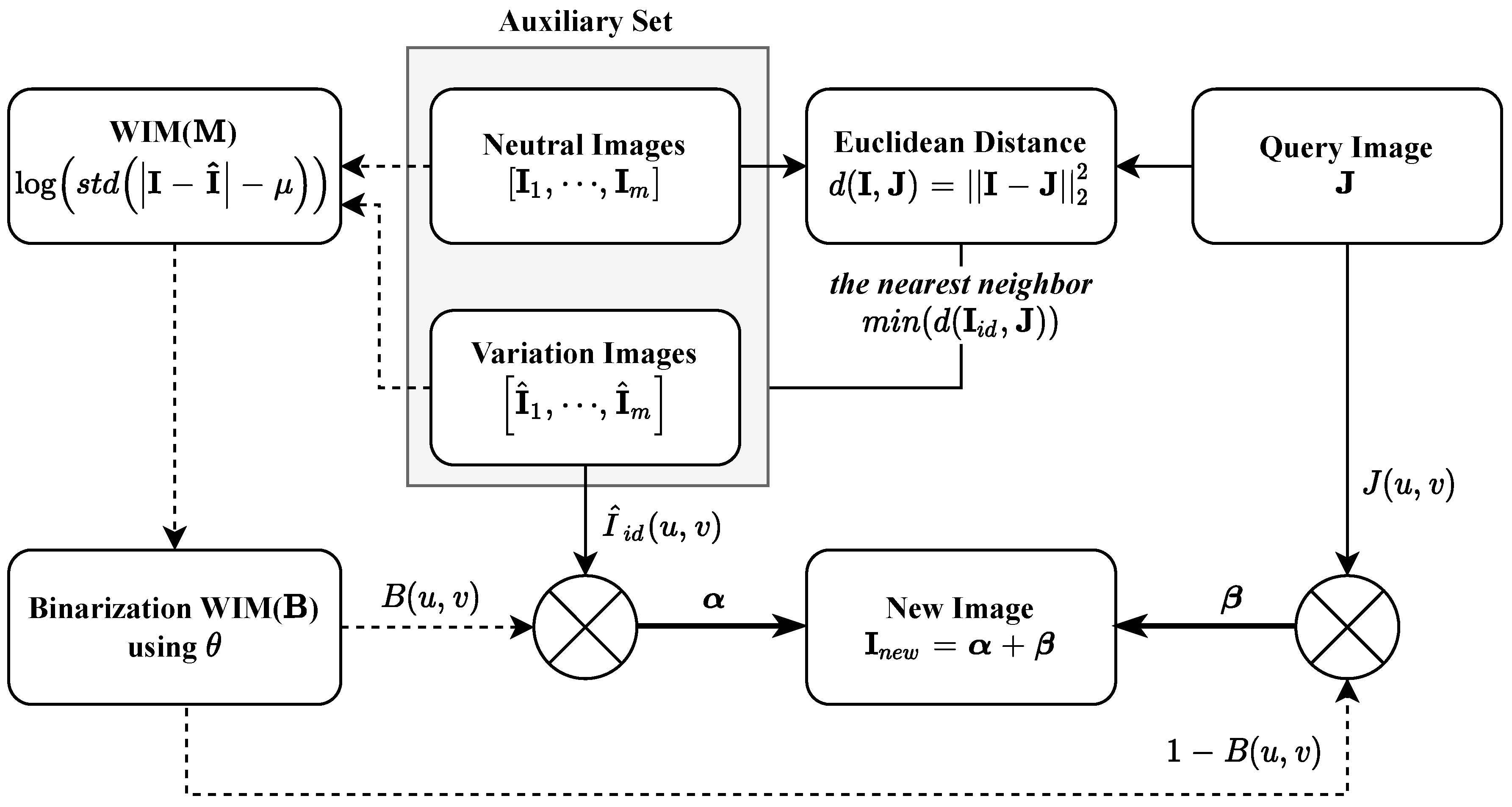
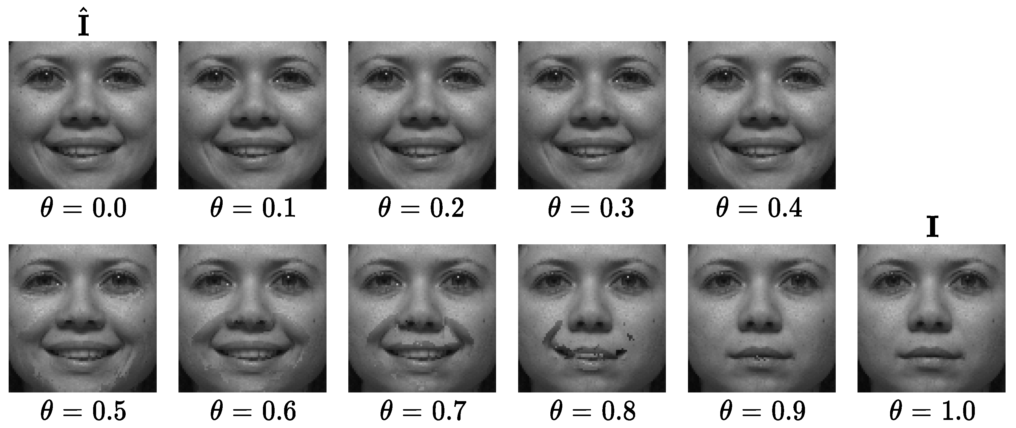
2.2. Generation of New Images from a Query Image

The new image (${\mathbf{I}}_{new}$) can be generated from a query image ($\mathbf{J}$) as follows:

$$I_{new}(u,v)=(1-\mathcal{B}(u,v))J(u,v)+\mathcal{B}(u,v)\widehat{J}(u,v).$$

(6)

Unlike during the phase of B-WIM extraction, a variational image ($\widehat{\mathbf{J}}$) derived from $\mathbf{J}$ cannot be obtained in the phase of image generation. Therefore, $\widehat{\mathbf{J}}$ must be replaced with another image in a separate auxiliary set. In WIM, the mean image for each variation in the auxiliary set is used as $\widehat{\mathbf{J}}$. Although it can be applied equally to all query images, morphological elements may be lost if the variation’s own changes are large. For example, mufflers can be worn in various ways depending on a person’s personality. Moreover, the designs of mufflers are also very diverse. Therefore, the mean image cannot preserve the form of all mufflers.

In this study, we select the neutral image (i.e., nearest neighbor) of the auxiliary set with a minimum Euclidean distance (L2-norm) from the query image based on the whole pixel [28].

$$d(\mathbf{I},\mathbf{J})=\left|\right|\mathbf{I}-{\mathbf{J}\left|\right|}_2^2$$

(7)

Then, $\widehat{\mathbf{J}}$ is replaced by ${\widehat{\mathbf{I}}}_{id}$, derived from ${\mathbf{I}}_{id}$, where $id$ is the index with a minimum distance from $\mathbf{J}$($\min \left(d\right(\mathbf{I},\mathbf{J}\left)\right)$). Equation (6) is redefined as

$$I_{new}(u,v)\approx (1-\mathcal{B}(u,v))J(u,v)+\mathcal{B}(u,v){\widehat{I}}_{id}(u,v).$$

(8)

Finally, ${\mathbf{I}}_{new}$ is generated from Equation (8).

The overall procedure of the proposed method is summarized as follows:

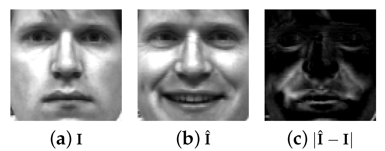
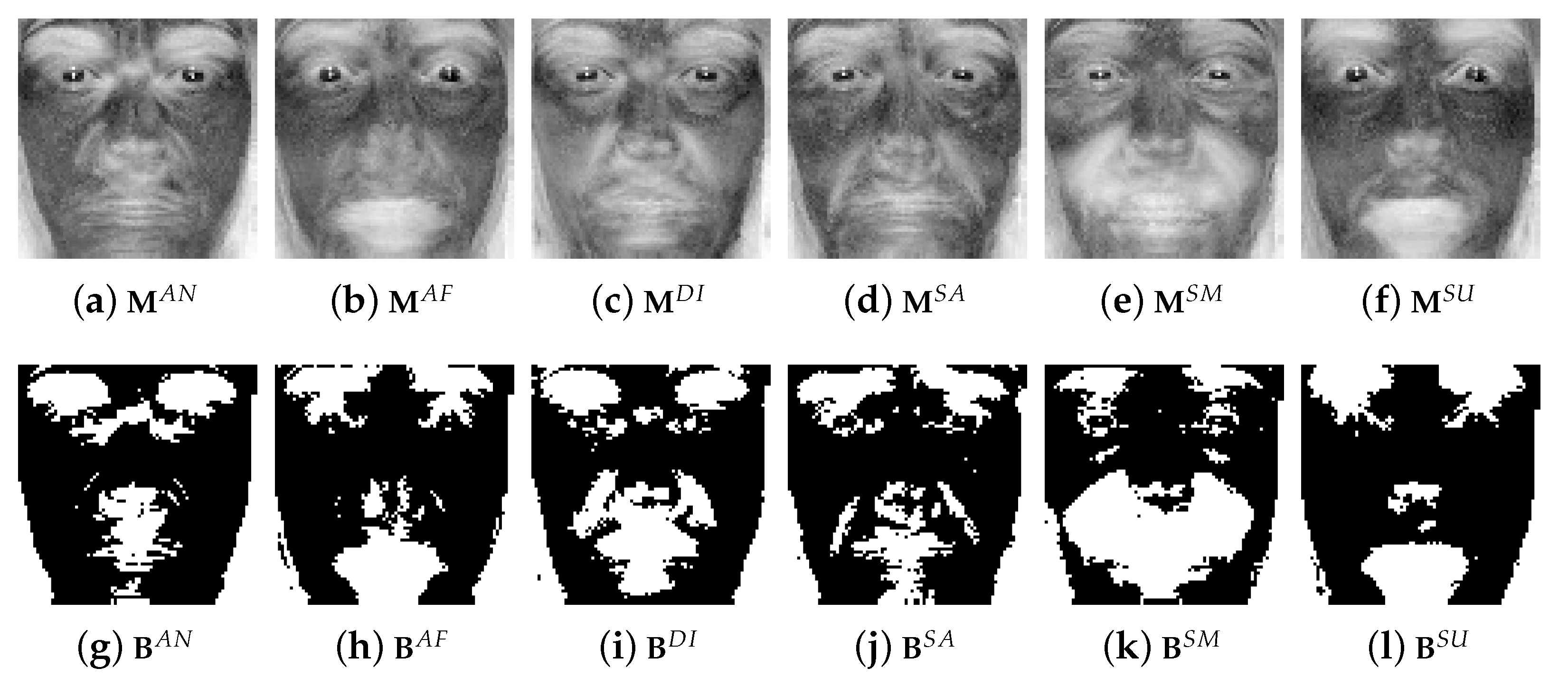
• Step 1: Extraction of the normalized WIM using log-scaled standard deviation of the absolute difference between $\mathbf{I}$ and $\widehat{\mathbf{I}}$ in the auxiliary set;
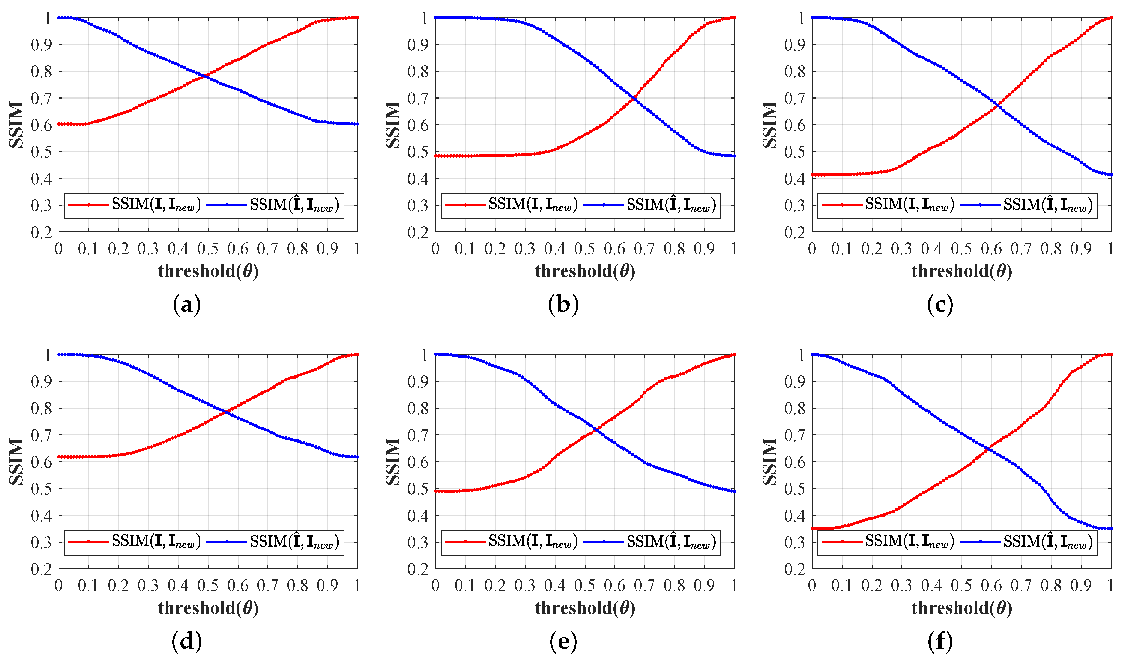
• Step 2: Binarization of WIM from threshold ($\theta$);
• Step 3: Selection of the index ($id$) of the nearest neighbor in the auxiliary set based on Euclidean distance with the query image; ($\min \left(\right||\mathbf{I}-\mathbf{J}|{|}_2^2)$)
• Step 4: Replacement of $\widehat{\mathbf{J}}$ with ${\widehat{\mathbf{I}}}_{id}$, derived from ${\mathbf{I}}_{id}$;
• Step 5: Generation of the new image (${\mathbf{I}}_{new}$).

3. Experiments

3.1. Database

In the experiment, all images were aligned to 80 × 80 pixels via affine transformation based on manually detected eye coordinates. Then, the image was compensated using histogram equalization [38].

We used the Bosphorus [32] and RaFD [39] databases in our face recognition experiments (

Table 1. Characteristics of each facial expression database.

Expression	Bosphorus	RaFD
Neutral	◯	◯
Afraid	◯	◯
Angry	◯	◯
Disgusted	◯	◯
Sad	◯	◯
Smiling (smiling)	◯	◯
Surprise (scream)	◯	◯
Contemptuous		◯
No. of subjects	58	67
No. of images per subject	7	8
Index of neutral face images	5	6
No. of testing images	348	469

). The Bosphorus database comprises images captured under seven different facial expression conditions from 58 subjects and includes various expressions, such as neutral, angry, disgusted, afraid, sad, smiling, and surprised. The neutral images (“indexed 5”) were selected to generate new images, and the remaining images were used for the face recognition test. The RaFD database contains 536 images captured from 67 subjects. Each subject provided images of eight facial expressions (i.e., neutral, angry, contemptuous, disgusted, afraid, sad, smiling, and surprised). We used a neutral image (“indexed 6”) to generate new images, and the remaining facial expression images were used for testing. Both databases applied practiced expressions using a Facial Action Coding System (FACS) [33] specialist. Furthermore, all subjects were tightly controlled through negative feedback to acquire the required activation of action units (AU).

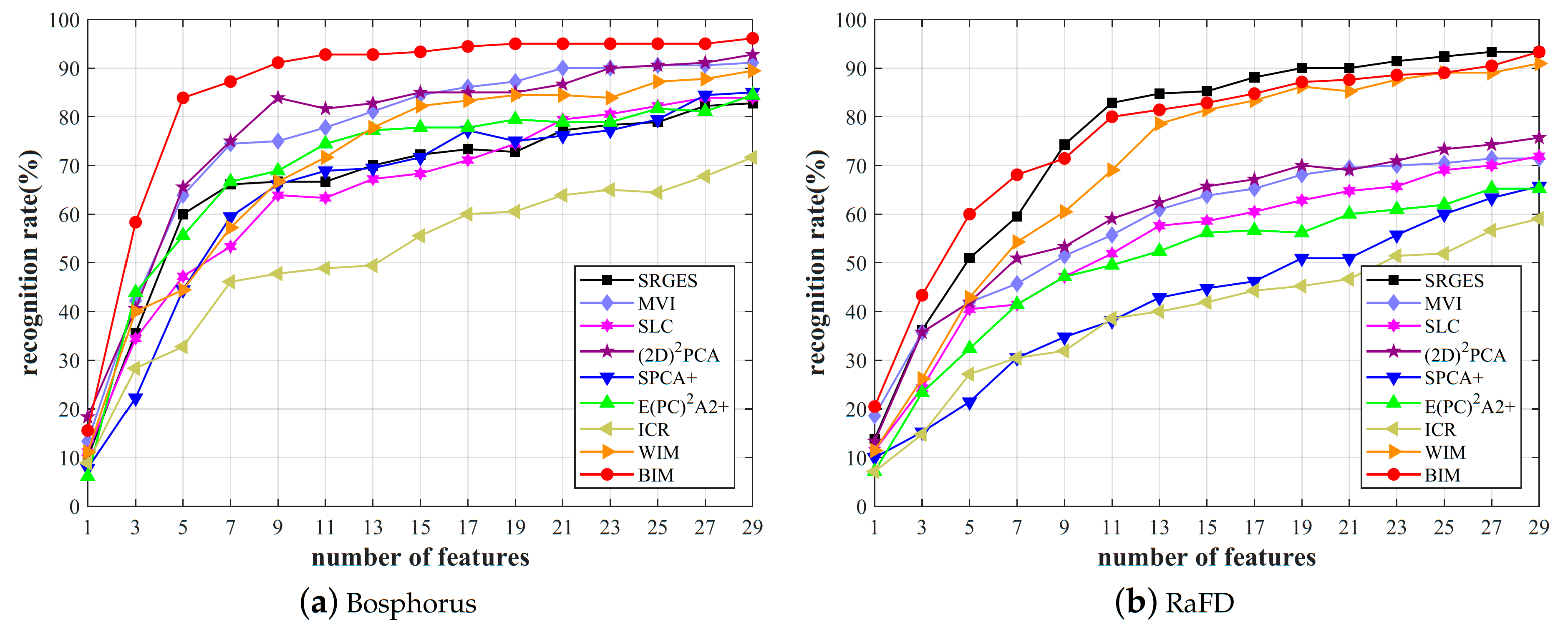
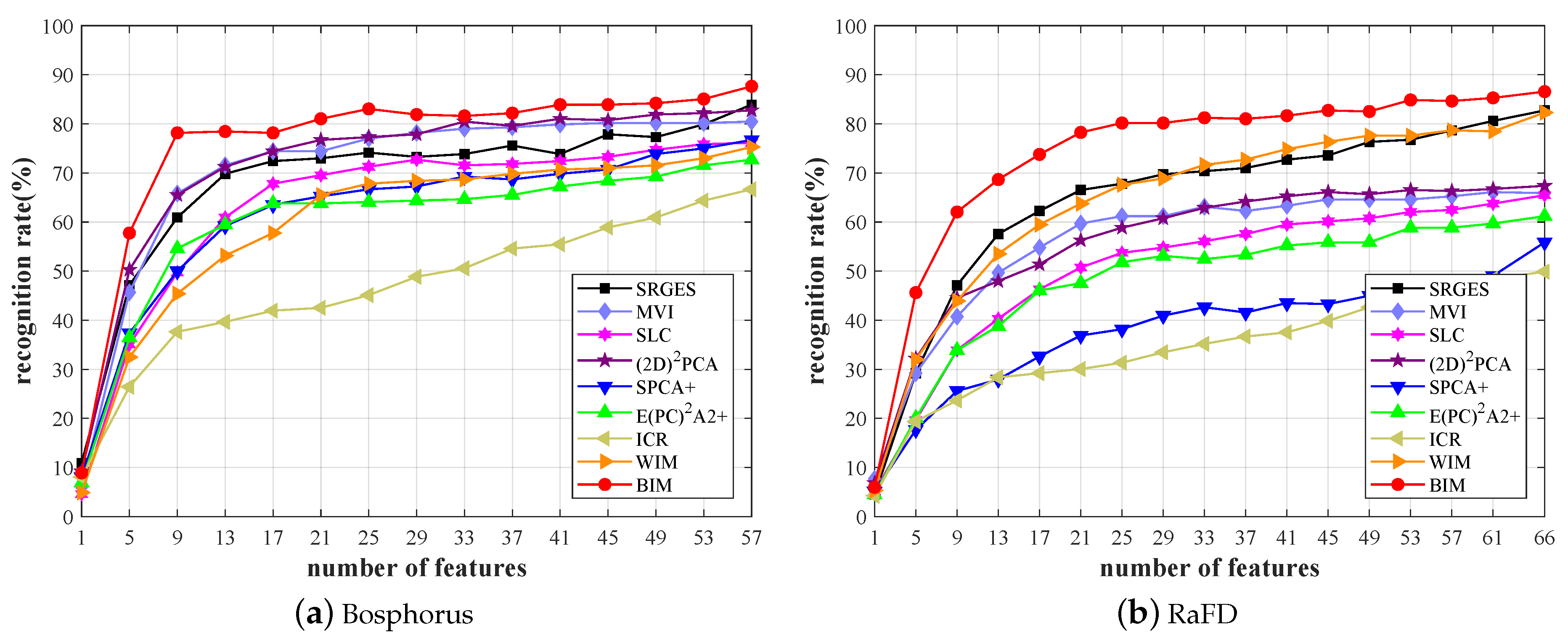
3.2. Face Recognition Results

We compared the proposed method with other methods dealing with the SSPP problem (i.e., WIM, ICR, E(${\mathrm{PC}}^2$)A+, SPCA+, ${\left(2\mathrm{D}\right)}^2$PCA, SLC, MVI, and SRGES methods). The proposed method, WIM, and SRGESgenerated as many images as the number of variations contained in the auxiliary set. With the ICR, the number of generated images depended on the k neighbors in the training set and the feature extraction method used by each database. In E(PC2)A+, the half-, first-, and second-order projected images of each neutral image were used as the training set. In SPCA+, seven images were enlarged from different n-order singular values for each neutral image in the training set. In ${\left(2\mathrm{D}\right)}^2$PCA, an image was generated using a two-directional PCA in the row and column directions of the 2D images. In SLC, 11 images from the neutral image were added to the training set, which included symmetric images and linear combinations of virtual images. In MVI, four low-resolution images (size $40\times 40$, $26\times 26$, $20\times 20$, and $16\times 16$) are generated from the neutral image and various scaling factors (i.e., 2, 3, 4, 5, respectively).

In this study, the face recognition performance of all methods was evaluated based on the given criteria. First, we measured the change in the face recognition rate according to the degree of variation in each database. Both databases contained similar facial expression variations, but they differed in the intensity of the facial expressions. In the Bosphorus database, the AUs were captured at their given peak intensity levels. In the RaFD database, there were large deviations in the intensities of expressions according to subject. Thus, the RaFD database was closer to the real world than the Bosphorus one. Second, the face recognition performance was analyzed according to unsupervised and supervised learning methods. An unsupervised learning-based PCA [24] and supervised learning-based discriminant common vector (DCV) [40] were used to extract the features for face recognition. PCA extracted $(\mathcal{N}+{\mathcal{N}}^{\prime }-1)$ features, including the number of images of training data ($\mathcal{N}$) and the number of enlarged images (${\mathcal{N}}^{\prime }$) from itself. DCV extracted $(c-1)$ features, where c was the total number of classes, regardless of the number of images. In the face recognition experiment, the recognition rates were measured using the maximum number of features extracted from each method. If a given set had been modeled properly, it could be expected to show high performance, regardless of the two methods. When evaluating the face recognition performance, the one nearest-neighbor rule was used with the $l_2$ norm as a classifier.

In this study, two protocols for face recognition were used [41]: “$ClosedSet$” and “$OpenSet$”, according to the auxiliary set. These are described as follows:

• $Closedset$: In this case, all images were collected under similar conditions. Thus, all images belonged to the same database. In the experiment, the database was divided into a face recognition set and an auxiliary set. The face recognition set consisted of training and test sets. Neutral images for each class used to generate images were included in the training set, and the remaining images containing only variations were used as the test set. This method had the same variations (“expression”) in both face recognition and auxiliary sets;
• $Openset$: This case used a separate auxiliary set from a given database to demonstrate the superiority of the proposed method. The training and test sets were collected under similar conditions. However, the auxiliary set was taken in environments different from those. The face recognition set was constructed in the same way as in the “$ClosedSet$” case, and neutral images were used to enlarge the others. Both face recognition and auxiliary sets included “expression” variations. However, the types of detailed variations could be different.

First, we divided the given databases into face recognition and auxiliary sets. A total of 30 subjects from all subjects in each database were used for the face recognition set, and the others were used for the auxiliary set. Among the 210 and 240 images for 30 subjects in the Bosphorus and RaFD databases, respectively, neutral images were used as training data to construct PCA and DCV feature spaces for face recognition, and variational images were generated using the proposed methods from these images to enlarge the training set.

Table 2. Face recognition results in $ClosedSet$ protocol.

Method	Bosphorus		RaFD
	PCA	DCV	PCA	DCV
B-WIM	95.56%	96.11%	90.48%	93.33%
WIM [31]	91.11%	89.44%	84.29%	90.95%
ICR [28]	93.89%	71.67%	76.67%	59.05%
E(PC)${}^2$A2+ [21]	92.78%	84.44%	65.71%	65.24%
SPCA+ [25]	88.89%	85.00%	55.71%	65.71%
(2D)${}^2$PCA [26]	91.11%	92.78%	76.19%	75.71%
SLC [27]	91.11%	83.89%	75.24%	71.90%
MVI [29]	92.78%	90.56%	74.76%	75.24%
SRGES [30]	92.22%	82.78%	77.62%	93.33%

shows the face recognition results for the “$ClosedSet$” protocol. In the experimental results, the proposed method, WIM, and (2D)${}^2$PCA presented similar facial-recognition results within the same database, regardless of the feature-extraction manner. The other methods had a face recognition rate difference of up to 21.11% between each manner. Additionally, the proposed method and WIM showed high performance in the face recognition results according to the degree of variation by database. For the rest of the methods, the face recognition performance decreased by more than 15.87∼33.17% as the degree of variation increased. Figure 6 shows the recognition rates for a different number of DCV features. The proposed method gives a recognition rate of 96.11% and 93.33%, with 29 features for the Bosphorus and RaFD databases, respectively. As can be seen from Figure 6, the proposed method shows a comparable or better recognition performance to the other methods, regardless of the number of features. Finally, we confirmed that the proposed method was excellent in the absolute comparison of face recognition rates for both databases. Because the proposed method consistently showed high face recognition performance regardless of the various criteria, it could be inferred that a new image was generated by reflecting the various variations from the given neutral images.

Generally, the basic emotion group consists of angry, disgusted, afraid, sad, smiling, and surprised [42]. For the “$OpenSet$” protocol, the auxiliary set containing six defined facial expressions consists of the AR [43], CK+ [44], Jaffe [45], PF07 [46], and Yale [47] databases. Additionally, it included various races and genders. To measure the degree of change from the variations, only subjects without glasses (occlusion) were used to construct the auxiliary set. The selected subjects had images of both neutral and facial expressions.

The AR database contained images from 85 subjects (37 males and 48 females) of different races [43]. We selected four facial expressions: neutral, angry, smiling, and screaming. The CK+ database contained 84 subjects from many different races. Image sequences contained changes in facial expressions over time. The neutral image at the start time and the facial expression image at the end time comprised the auxiliary set. We used seven facial expressions (i.e., neutral, angry, afraid, disgusted, sad, smiling, and surprised), except for “contemptuous.” The Jaffe database included 10 subjects (only females) of Asian ethnic groups. Seven facial expressions of each subject were taken (e.g., neutral, angry, afraid, disgusted, sad, smiling, and surprised). The PF07 database contained the images of 200 subjects (100 males and 100 females) of Asian ethnic groups, all of whom provided four images with different facial expression conditions (i.e., neutral, angry, smiling, and surprised). The Yale database included 15 subjects (14 males and a female) of many different races. We used four facial expressions (i.e., neutral, sad, smiling, and surprised), excluding those with eyes closed or winking (

Table 3. Facial expressions in each database in the auxiliary set.

Expressions	AR	CK+	Jaffe	PF07	Yale
Neutral	◯	◯	◯	◯	◯
Afraid		◯	◯
Angry	◯	◯	◯	◯
Disgusted		◯	◯
Sad		◯	◯		◯
Smiling (smiling)	◯	◯	◯	◯	◯
Surprised (screaming)	◯	◯	◯	◯	◯

).

Table 4. Face recognition results in $OpenSet$ protocol.

Method	Bosphorus		RaFD
	PCA	DCV	PCA	DCV
B-WIM	87.64%	88.51%	81.88%	87.21%
WIM [31]	86.49%	75.29%	76.12%	82.30%
ICR [28]	83.91%	66.67%	66.52%	49.89%
E(PC)${}^2$A2+ [21]	83.62%	72.70%	58.85%	61.19%
SPCA+ [25]	78.16%	76.72%	47.33%	55.86%
(2D)${}^2$PCA [26]	81.32%	82.76%	67.59%	67.38%
SLC [27]	82.18%	76.15%	71.86%	65.46%
MVI [29]	82.76%	83.05%	65.88%	69.08%
SRGES [30]	81.90%	83.91%	73.13%	82.73%

shows the face recognition results with a separate auxiliary set. Because the auxiliary set was constructed from separate databases, the face recognition experiment used images of all the subjects contained in each database.

Depending on the degree of variation, the differences in face recognition rates were measured in the order of the proposed method: ($5.77\%$), SRGES ($8.76\%$), WIM ($10.37\%$), SLC ($10.69\%$), (2D)${}^2$PCA ($15.38\%$), MVI ($16.87\%$), ICR ($17.38\%$), E(PC)${}^2$A2+ ($24.77\%$), and SPCA+ ($30.83\%$). For the criteria, the proposed method and SLC maintained high performance, whereas the remaining methods showed differences in face recognition performance. Generally, the proposed method showed the highest face recognition rates. Figure 7 shows the recognition rates for a different number of DCV features. The proposed method gives a recognition rate of 88.51% with 57 features and 87.21% with 66 features for the Bosphorus and RaFD databases, respectively. As can be seen from Figure 7, the proposed method shows the best recognition performance compared to the other methods for all number of features. This experiment also confirmed the superiority of the proposed method for each criterion.

On the other hand, from the results of Table 2 and Table 4, it can be seen that the recognition rate in the “$ClosedSet$” protocol was about 10% higher than that in the “$OpenSet$” protocol. It is generally known that face recognition performance decreases as the number of subjects to be recognized increases [48]. In our experiment, however, we think the main reason for the difference between the results of Table 2 and Table 4 is that, in the “$ClosedSet$” protocol, the images included in the auxiliaries set had homogeneous characteristics, because they were taken under similar conditions of resolution, camera type, lighting conditions, etc. However, in the “$OpenSet$” protocol, the auxiliary set comprised images from various kinds of databases, which differ from the query images.

4. Discussion and Conclusions

Building a face recognition system that works robustly in various environments involves difficulties in securing the data needed to learn recognition algorithms. Moreover, large-scale face recognition applications typically use databases that contain SSPPs. A single image is not sufficiently representative for face recognition. The SSPP problem makes using the feature extraction method in a supervised manner quite difficult, because the interclass variations are unknown. To overcome this, several methods have been proposed. However, there have been limitations in that these methods did not reflect facial characteristics that could have various variations.

We proposed an image generation method that uses a B-WIM that leverages the fact that the pixels of specific parts of the neutral face image vary significantly compared with other areas when there is an environmental variation in face recognition. The B-WIM statistically reflects the change in individual pixel values caused by the variation from the neutral and variational images included in the auxiliary set. For a given query image (neutral image), the proposed method creates a new variational image that reflects the characteristics of the variation while maintaining the unique characteristics of the face in the query image based on B-WIM. Through this, a training dataset containing only one sample per person can be made into a richer set that includes variational images for each person, further improving the performance of the face recognition system.

The proposed method has the following advantages. The proposed method does not require a large amount of computation or a large dataset for creating new images. When the number of pixels in an image is n, while SPCA+ has the complexity of $O\left(n^2\right)$, the complexity of the proposed method is $O\left(n\right)$. Some methods, such as ICR, E(${\mathrm{PC}}^2$)A+, ${\left(2\mathrm{D}\right)}^2$PCA, SLC, and MVI, require similar computations as the proposed method but do not address specific variations. In contrast, the proposed method generates high-quality variational images for query images in real-time, effectively improving the performance of existing face recognition systems at a low cost. Face recognition experiments using Bosphorus and RaFD databases showed that the proposed method outperformed the existing methods for solving the SSPP problem. In addition to general facial recognition algorithms, images generated using the proposed method can be utilized in the study of various facial images, including the fake image detection algorithms [49,50].

On the other hand, by comparing the recognition rates for two protocols of face recognition, “$ClosedSet$” and “$OpenSet$,” we found that the quality of the image created using the proposed method was affected by the images included in the auxiliary set. Although the proposed method can effectively generate new images for a specific variation, it does not control the degree of variation or handle more than two variations simultaneously. It is expected that the small sample-size problems, including the SSPP problem, can be solved more effectively by subdividing the degree of variation within the proposed method’s algorithmic structure and applying the interpolation maps for two or more types of variations together. We leave these problems to future works.

References

1. Kortli, Y.; Jridi, M.; Al Falou, A.; Atri, M. Face recognition systems: A Survey. Sensors 2020, 20, 342. [Google Scholar] [CrossRef] [Green Version]
2. Choi, S.I.; Lee, Y.; Lee, M. Face Recognition in SSPP Problem Using Face Relighting Based on Coupled Bilinear Model. Sensors 2019, 19, 43. [Google Scholar] [CrossRef] [Green Version]
3. Cao, Q.; Shen, L.; Xie, W.; Parkhi, O.M.; Zisserman, A. Vggface2: A dataset for recognising faces across pose and age. In Proceedings of the 2018 13th IEEE International Conference on Automatic Face & Gesture Recognition (FG 2018), Xi’an, China, 15–19 May 2018; pp. 67–74. [Google Scholar]
4. Panetta, K.; Wan, Q.; Agaian, S.; Rajeev, S.; Kamath, S.; Rajendran, R.; Rao, S.; Kaszowska, A.; Taylor, H.; Samani, A.; et al. A comprehensive database for benchmarking imaging systems. IEEE Trans. Pattern Anal. Mach. Intell. 2018, 42, 509–520. [Google Scholar] [CrossRef]
5. Bansal, A.; Nanduri, A.; Castillo, C.D.; Ranjan, R.; Chellappa, R. Umdfaces: An annotated face dataset for training deep networks. In Proceedings of the 2017 IEEE International Joint Conference on Biometrics (IJCB), Denver, CO, USA, 1–4 October 2017; pp. 464–473. [Google Scholar]
6. Kemelmacher-Shlizerman, I.; Seitz, S.M.; Miller, D.; Brossard, E. The megaface benchmark: 1 million faces for recognition at scale. In Proceedings of the IEEE Conference on Computer Vision and Pattern Recognition, Las Vegas, NV, USA, 27–30 June 2016; pp. 4873–4882. [Google Scholar]
7. Huang, G.B.; Mattar, M.; Berg, T.; Learned-Miller, E. Labeled Faces in the Wild: A Database for Studying Face Recognition in Unconstrained Environments. 2008. Available online: http://vis-www.cs.umass.edu/lfw (accessed on 1 September 2020).
8. Huang, G.B.; Learned-Miller, E. Labeled Faces in the Wild: Updates and New Reporting Procedures; Technical Report UM-CS-2014-003; Department of Computer Science, University of Massachusetts Amherst: Amherst, MA, USA, 2014. [Google Scholar]
9. Tan, X.; Chen, S.; Zhou, Z.H.; Zhang, F. Face recognition from a single image per person: A survey. Pattern Recognit. 2006, 39, 1725–1745. [Google Scholar] [CrossRef] [Green Version]
10. Ríos-Sánchez, B.; Costa-da Silva, D.; Martín-Yuste, N.; Sánchez-Ávila, C. Deep Learning for Facial Recognition on Single Sample per Person Scenarios with Varied Capturing Conditions. Appl. Sci. 2019, 9, 5474. [Google Scholar] [CrossRef] [Green Version]
11. Noyes, E.; Jenkins, R. Deliberate disguise in face identification. J. Exp. Psychol. Appl. 2019, 25, 280. [Google Scholar] [CrossRef] [Green Version]
12. Demleitner, N.V. Witness Protection in Criminal Cases: Anonymity, Disguise or Other Options? Am. J. Comp. Law 1998, 46, 641–664. [Google Scholar] [CrossRef]
13. Wang, F.; Cheng, J.; Liu, W.; Liu, H. Additive margin softmax for face verification. IEEE Signal Process. Lett. 2018, 25, 926–930. [Google Scholar] [CrossRef] [Green Version]
14. Deng, J.; Guo, J.; Xue, N.; Zafeiriou, S. Arcface: Additive angular margin loss for deep face recognition. In Proceedings of the IEEE Conference on Computer Vision and Pattern Recognition, Long Beach, CA, USA, 15–20 June 2019; pp. 4690–4699. [Google Scholar]
15. Wang, H.; Wang, Y.; Zhou, Z.; Ji, X.; Gong, D.; Zhou, J.; Li, Z.; Liu, W. Cosface: Large margin cosine loss for deep face recognition. In Proceedings of the IEEE Conference on Computer Vision and Pattern Recognition, Salt Lake City, UT, USA, 18–22 June 2018; pp. 5265–5274. [Google Scholar]
16. Zheng, Y.; Pal, D.K.; Savvides, M. Ring loss: Convex feature normalization for face recognition. In Proceedings of the IEEE Conference on Computer Vision and Pattern Recognition, Salt Lake City, UT, USA, 18–22 June 2018; pp. 5089–5097. [Google Scholar]
17. Coccia, M.; Watts, J. A theory of the evolution of technology: Technological parasitism and the implications for innovation magement. J. Eng. Technol. Manag. 2020, 55, 101552. [Google Scholar] [CrossRef]
18. Coccia, M. Sources of technological innovation: Radical and incremental innovation problem-driven to support competitive advantage of firms. Technol. Anal. Strateg. Manag. 2017, 29, 1048–1061. [Google Scholar] [CrossRef]
19. Arthur, W.B. The Nature of Technology: What It Is and How It Evolves; Simon and Schuster: New York City, NY, USA, 2009. [Google Scholar]
20. Arthur, W.B.; Polak, W. The evolution of technology within a simple computer model. Complexity 2006, 11, 23–31. [Google Scholar] [CrossRef]
21. Chen, S.; Zhang, D.; Zhou, Z.H. Enhanced (PC)2A for face recognition with one training image per person. Pattern Recognit. Lett. 2004, 25, 1173–1181. [Google Scholar] [CrossRef]
22. Wu, J.; Zhou, Z.H. Face recognition with one training image per person. Pattern Recognit. Lett. 2002, 23, 1711–1719. [Google Scholar] [CrossRef]
23. Zhang, D.; Zhou, Z.H. (2D)2PCA: Two-directional two-dimensional PCA for efficient face representation and recognition. Neurocomputing 2005, 69, 224–231. [Google Scholar] [CrossRef]
24. Turk, M.; Pentland, A. Eigenfaces for recognition. J. Cogn. Neurosci. 1991, 3, 71–86. [Google Scholar] [CrossRef]
25. Zhang, D.; Chen, S.; Zhou, Z.H. A new face recognition method based on SVD perturbation for single example image per person. Appl. Math. Comput. 2005, 163, 895–907. [Google Scholar] [CrossRef] [Green Version]
26. Xu, Y.; Zhu, X.; Li, Z.; Liu, G.; Lu, Y.; Liu, H. Using the original and ‘symmetrical face’ training samples to perform representation based two-step face recognition. Pattern Recognit. 2013, 46, 1151–1158. [Google Scholar] [CrossRef]
27. Zhang, T.; Li, X.; Guo, R.Z. Producing virtual face images for single sample face recognition. Opt.-Int. J. Light Electron Opt. 2014, 125, 5017–5024. [Google Scholar] [CrossRef]
28. Li, Q.; Wang, H.J.; You, J.; Li, Z.M.; Li, J.X. Enlarge the training set based on inter-class relationship for face recognition from one image per person. PLoS ONE 2013, 8, e68539. [Google Scholar] [CrossRef] [Green Version]
29. Moon, H.M.; Kim, M.G.; Shin, J.H.; Pan, S.B. Multiresolution face recognition through virtual faces generation using a single image for one person. Wirel. Commun. Mob. Comput. 2018, 2018. [Google Scholar] [CrossRef] [Green Version]
30. Ding, Y.; Qi, L.; Tie, Y.; Liang, C.; Wang, Z. Single sample per person face recognition based on sparse representation with extended generic set. In Proceedings of the 2018 International Conference on Cyber-Enabled Distributed Computing and Knowledge Discovery (CyberC), Zhengzhou, China, 18–20 October 2018; pp. 37–375. [Google Scholar]
31. Lee, Y.; Kang, J. Occlusion Images Generation from Occlusion-Free Images for Criminals Identification based on Artificial Intelligence Using Image. Int. J. Eng. Technol. 2018, 7, 161–164. [Google Scholar]
32. Savran, A.; Alyüz, N.; Dibeklioğlu, H.; Çeliktutan, O.; Gökberk, B.; Sankur, B.; Akarun, L. Bosphorus database for 3D face analysis. In European Workshop on Biometrics and Identity Management; Springer: Berlin/Heidelberg, Germany, 2008; pp. 47–56. [Google Scholar]
33. Friesen, E.; Ekman, P. Facial Action Coding System: A Technique for the Measurement of Facial Movement; Consulting Psychologists Press: City of Palo Alto, CA, USA, 1978. [Google Scholar]
34. Scheve, T. How Many Muscles Does It Take to Smile? How Stuff Works Science. June 2009, Volume 2. Available online: https://science.howstuffworks.com/life/inside-the-mind/emotions/muscles-smile.htm (accessed on 1 September 2020).
35. Waller, B.M.; Cray, J.J., Jr.; Burrows, A.M. Selection for universal facial emotion. Emotion 2008, 8, 435. [Google Scholar] [CrossRef] [Green Version]
36. Wang, Z.; Bovik, A.C.; Sheikh, H.R.; Simoncelli, E.P. Image quality assessment: From error visibility to structural similarity. IEEE Trans. Image Process. 2004, 13, 600–612. [Google Scholar] [CrossRef] [Green Version]
37. Renieblas, G.P.; Nogués, A.T.; González, A.M.; León, N.G.; Del Castillo, E.G. Structural similarity index family for image quality assessment in radiological images. J. Med. Imaging 2017, 4, 035501. [Google Scholar] [CrossRef]
38. Gonzalez, R.C.; Woods, R.E. Digital Image Processing; Prentice Hall: Upper Saddle River, NJ, USA, 2002. [Google Scholar]
39. Langner, O.; Dotsch, R.; Bijlstra, G.; Wigboldus, D.H.; Hawk, S.T.; Van Knippenberg, A. Presentation and validation of the Radboud Faces Database. Cogn. Emot. 2010, 24, 1377–1388. [Google Scholar] [CrossRef]
40. Cevikalp, H.; Neamtu, M.; Wilkes, M.; Barkana, A. Discriminative common vectors for face recognition. IEEE Trans. Pattern Anal. Mach. Intell. 2005, 27, 4–13. [Google Scholar] [CrossRef]
41. Liu, W.; Wen, Y.; Yu, Z.; Li, M.; Raj, B.; Song, L. Sphereface: Deep hypersphere embedding for face recognition. In Proceedings of the IEEE Conference on Computer Vision and Pattern Recognition (CVPR), Honolulu, HI, USA, 21–26 July 2017; Volume 1, p. 1. [Google Scholar]
42. Du, S.; Tao, Y.; Martinez, A.M. Compound facial expressions of emotion. Proc. Natl. Acad. Sci. USA 2014, 111, E1454–E1462. [Google Scholar]
43. Martınez, A.; Benavente, R. The AR face database. Rapp. Tech. 1998, 24. Available online: http://www2.ece.ohio-state.edu/~aleix/ARdatabase (accessed on 1 September 2020).
44. Lucey, P.; Cohn, J.F.; Kanade, T.; Saragih, J.; Ambadar, Z.; Matthews, I. The extended cohn-kanade dataset (ck+): A complete dataset for action unit and emotion-specified expression. In Proceedings of the 2010 IEEE Computer Society Conference on Computer Vision and Pattern Recognition Workshops (CVPRW), San Francisco, CA, USA, 13–18 June 2010; pp. 94–101. [Google Scholar]
45. Lyons, M.; Akamatsu, S.; Kamachi, M.; Gyoba, J. Coding facial expressions with gabor wavelets. In Proceedings of the 1998 Third IEEE International Conference on Automatic Face and Gesture Recognition, Nara, Japan, 14–16 April 1998; pp. 200–205. [Google Scholar]
46. Lee, H.S.; Park, S.; Kang, B.N.; Shin, J.; Lee, J.Y.; Je, H.; Jun, B.; Kim, D. The POSTECH face database (PF07) and performance evaluation. In Proceedings of the 8th IEEE International Conference on Automatic Face & Gesture Recognition (2008 FG’08), Amsterdam, The Netherlands, 17–19 September 2008; pp. 1–6. [Google Scholar]
47. Georghiades, A. Yale Face Database. Center for Computational Vision and Control at Yale University, 1997. Available online: http://cvc.cs.yale.edu/cvc/projects/yalefaces/yalefaces.html (accessed on 1 September 2020).
48. Shamir, L. Evaluation of face datasets as tools for assessing the performance of face recognition methods. Int. J. Comput. Vis. 2008, 79, 225. [Google Scholar]
49. Dang, L.M.; Hassan, S.I.; Im, S.; Moon, H. Face image manipulation detection based on a convolutional neural network. Expert Syst. Appl. 2019, 129, 156–168. [Google Scholar] [CrossRef]
50. He, M. Distinguish computer generated and digital images: A CNN solution. Concurr. Comput. Pract. Exp. 2019, 31, e4788. [Google Scholar] [CrossRef]
Figure 1. Overall procedure of the proposed method.
Applsci 10 06659 g001
Figure 2. (a) Neutral image; (b) variational image; (c) absolute difference between neutral and variational image.
Applsci 10 06659 g002
Figure 3. Weighted interpolation maps ( M ) and binary weighted interpolation maps ( B ) for facial expressions. ( A N : angry, A F : afraid, D I : disgusted, S A : sad, S M : smiling, S U : surprised).
Applsci 10 06659 g003
Figure 4. Structural similarity (SSIM) results for each variation (a) angry; (b) afraid; (c) disgusted; (d) sad; (e) smiling; (f) surprised.
Applsci 10 06659 g004
Figure 5. Generated images from I and I ^ for each threshold ( θ ).
Applsci 10 06659 g005
Figure 6. Face recognition results for a various number of DCV features in “ C l o s e d S e t ” protocol.
Applsci 10 06659 g006
Figure 7. Face recognition results for a various number of DCV features in “ O p e n S e t ” protocol.
Applsci 10 06659 g007