Article

Hybrid Harmony Search-Simulated Annealing Algorithm for Location-Inventory-Routing Problem in Supply Chain Network Design with Defect and Non-Defect Items

1
Department of Mathematics, Faculty of Science, Universiti Putra Malaysia, Serdang 43400, Selangor, Malaysia
2
Centre for Mathematical Sciences, Universiti Malaysia Pahang, Lebuhraya Tun Razak, Gambang, Kuantan 26300, Pahang, Malaysia
3
Laboratory of Computational Statistics and Operations Research, Institute for Mathematical Research, Universiti Putra Malaysia, Serdang 43400, Selangor, Malaysia
4
Nottingham University Business School, University of Nottingham Malaysia, Semenyih 43500, Selangor, Malaysia
*
Author to whom correspondence should be addressed.
Appl. Sci. 2020, 10(18), 6625; https://doi.org/10.3390/app10186625
Submission received: 30 July 2020 / Revised: 15 September 2020 / Accepted: 19 September 2020 / Published: 22 September 2020

Abstract

:
This paper considers a location-inventory-routing problem (LIRP) that integrates the strategic, tactical, and operational decision planning in supply chain network design. Both defect and non-defect items of returned products are considered in the cost of reverse logistics based on the economic production quantity model. The objective of the LIRP is to minimize the total cost of location-allocation of established depots, the cost of inventory, including production setup and holding cost, as well as the cost of travelled distance by the vehicles between the open depots and assigned customers. A Hybrid Harmony Search-Simulated Annealing (HS-SA) algorithm is proposed in this paper. This algorithm incorporates the dynamic values of harmony memory considering rate and pitch adjustment rate with the local optimization techniques to hybridize with the idea of probabilistic acceptance rule from simulated annealing, to avoid the local extreme points. Computational experiments on popular benchmark data sets show that the proposed hybrid HS-SA algorithm outperforms a standard HS and an improved HS for all cases.

1. Introduction

The need for designing networks in a supply chain has been attracting a lot of attention in recent years; a result of the booming development of industrial commerce. A practice in traditional commerce is that customers can return the unsatisfactory products they bought within a given certain period of time. This process is called the reverse logistics by which the products are returned for proper planning of their disposal [1]. Reverse logistics can also be defined as the process of moving goods for capturing value. Efficient reverse logistics can reduce cost especially transportation cost, shipping cost, and inventory cost. Besides that, it also improves the service by offering a fast response to the demands and returns from customers. By implementing reverse logistics in supply chain network design, the expectation of a gain in both profit and increased customer retention can be expected, benefiting both from the economic and social factor of the economy respectively [2].
Reverse logistics is necessary for various reasons; such as the increasing trend in customers’ returns, product lifecycles, and demanding customers [3]. To maintain a high level of customer satisfaction and quickly respond to the complaints, some industries are willing to handle those returns on their own and thus strive to provide an efficient logistics system to accommodate this. Hence, one can argue that it is necessary for the reverse logistics network and logistics process to be integrated. Nowadays, a large number of organizations are experiencing high volumes of product returns. Managing product returns in reverse logistics depends on detailed planning, especially when the volume of return flow had increased considerably [4]. The returned products can be re-entered into the market to be resold either with or without some refurbish process depending on the condition of the products. Returned products can be categorized into two categories which are defect or non-defect products. The non-defect products will be re-sold in the next batch while the defect products will need to go through the process of refurbishing before re-entering the market [5].
In supply chain network design, besides facility location and vehicle routing, inventory control is also considered an important part of the whole process of optimization. Designing a distribution network consists of the three sub-problems which is essential to drive the key performance for the overall productivity and profitability. Looking at previous works from literature, most of the studies done focused on the integration of only two sub-problems such as location-routing problem (LRP), Inventory-Routing Problem (IRP), or Location-Inventory Problem (LIP). We found work on the integration of all three sub-problems, i.e., Location-Inventory-Routing Problem (LIRP) to be very limited especially those utilising the Economic Production Quantity (EPQ) model. There is a body of literature with regards to the EOQ model. The EOQ model determines the optimal order quantity a company should purchase from other companies to minimize inventory cost. On the other hand, the EPQ model determines the optimal production quantity for manufacturing. The main difference between these two models is that the EPQ model assumes the company will produce its own quantity, therefore the orders are available in an incremental manner while the products are being produced. While the EOQ model assumes the order quantity arrives complete and immediately after ordering, meaning that the parts are produced by another company and are ready to be shipped when the order is made.
Since the EPQ model is less researched despite being a practice of most companies in the industry, we propose the LIRP utilizes the EPQ model for defect and non-defect items in reverse logistics. The problem is solved by a hybrid harmony search-simulated annealing (HS-SA) algorithm. The proposed algorithm incorporates the dynamic values of harmony memory considering rate (HMCR) and pitch adjustment rate (PAR) with the local optimization techniques from a HS, to hybridize with the idea of probabilistic acceptance rule from the SA to deal with premature convergence. Computational experiments on the popular benchmark dataset of Perl, Gaskell, and Christofides show that the proposed algorithm outperformed a standard HS and an improved HS for all cases.
This study is the extension of the research from [6,7]. The idea of solving the vehicle routing problem (VRP) using a standard HS algorithm is first proposed in [6]. The problem is further extended into the LRP in [7]. The HS in [6] solved the VRP using four local search techniques with fixed values of HMCR and PAR. In [7], they introduced the dynamic values of HMCR and PAR to solve the LRP. In this paper, we extended the methodology in [7] to solve the LIRP by adding two popular local search methods: 2-opt and 3-opt, as the local optimization techniques. The proposed HS is further enhanced by hybridizing it with SA with the implementation of probabilistic acceptance rule during the improvisation procedure of the HS.
The remainders of the paper are organized as follows: the literature review of supply chain network design is presented in Section 2. The mathematical formulation of the LIRP with EPQ model is given in Section 3. Section 4 describes the framework and procedures of the proposed hybrid HS-SA algorithm. The computational experiments on three sets of popular benchmark datasets are performed, and the results are discussed in Section 5. Lastly, the conclusions and future direction are given in Section 6.

2. Literature Review

The warehouse LRP (WLRP) is first proposed by [8]. The problem is decomposed into three sub-problems: Multi-Depot Vehicle Routing Problem (MDVRP), Warehouse Location-Allocation Problem (WLAP), and Multi-Depot Routing Allocation Problem (MDRAP) and is solved using the heuristic approach. Some other studies divided the problem into two phases [9]. The first phase is a LAP and the VRP follows in the second phase. The problem is solved sequentially and iteratively by SA. Reference [10] discussed the capacitated LRP under disruption and implemented several approaches in problem-solving such as metaheuristic based on maximum-likelihood sampling method, route-allocation improvement, two-stage neighborhood search and SA.
A two-phase hybrid heuristic search approach for LRP is introduced in [11]. The problem is decomposed into LAP and VRP. For the construction of the location distribution, they proposed a Tabu Search (TS) to determine a good configuration of the facilities to be used. Meanwhile, an Ant Colony Algorithm (ACO) was used at the routing phase to obtain good routes for the given configuration. The combination of Particle Swarm Optimization (PSO) with several heuristic algorithms is called Hybrid PSO (HybPSO-LRP) and is introduced in [12]. They combined the Multiple Phase Neighborhood Search-Greedy Randomized Adaptive Search Procedure (MPNS-GRASP) algorithm, the Expending Neighborhood Search (ENS) strategy, and a Path Relinking (PR) strategy into the PSO. With the same approach used in [12], reference [13] combined the same techniques with the Honey Bee Mating Optimization (HBMO). They solved the problem using a hybrid HBMO for LRP (HBMO-LRP).
We found several studies on the integrated IRP from literature. For example, reference [14] solved a multi-objective coordination in a supply chain with three objective functions: maximizing the firm’s profit, minimizing vendor’s routing, and maximizing the average service level of buyers. They determined the vehicle routing, the router assigned and the amount delivered for each buyer. A HS algorithm is proposed due to the complexity of the problem. Considering the environmental impact, authors in [15] proposed a green IRP to minimize the total cost of inventory and routing, vehicle fixed cost, and emissions that are determined by load, distance, speed, and vehicle characteristics. They employed an exact method which is a Branch-and-Cut Algorithm (BCA) to add user cuts to the model and used a commercial solver to solve the linear programming relaxation problem. Similar to [16], they analyzed the benefits of collaborative energy use (CO2 emission) and perishability in IRP with uncertain demand. The authors minimized the cost of routing, based on fuel and wage cost, waste, driving time and inventory. The problem is solved by the ILOG-OPL development studio and CPLEX 12.6 optimization.
A new bi-objective mathematical model which takes into account the economic, social, and environmental issues in the distribution of perishable products with a specified expiration date in IRPs is considered in [17]. They focused on inventory and distribution costs for the first objective and then looked at social issues to shape the second objective by considering the rate of accidents for the vehicle and the number of expired products. The Torabi-Hassani method was used and included vehicle noise emission as a constraint. The integrated Production, Inventory, and Distribution Routing Problem (PIDRP) was developed and solved heuristically with two solutions approach [18]. In the first phase, they solved the Mixed-Integer Program (MIP) with CPLEX MIP solver and in the second phase, they solved an associated consolidation problem to handle the potential inefficiency of direct shipments involving routing and inventories by Extended Optimal Partitioning (EOP) procedure. This approach can simultaneously coordinate the production, inventory, and transportation operation in PIDRP. The two-step procedure is getting more attention in solving IRP, researchers in [19] performed a comparative analysis of a series of heuristics for manufacturing supply chain with a MIP formulation and two-step procedure development. The first step is to estimate the daily delivery quantities and followed by solving a VRP in the second step. A previously developed branch-and-price algorithm is used and the production decision and inventory flow balance were taken into account in the model.
Besides IRP, the integrated LIP is also gaining popularity. An optimization model for perishable products with fuzzy capacity and carbon emission constraints for integrated LIP is proposed by [20]. They formulated a Mixed-Integer Nonlinear Programming (MINP) and is solved by using two methods which are Hybrid Genetic Algorithm (HGA) and Hybrid HS (HHS). They found that HHS gave a better solution but needed higher computing time when compared to the HGA. The LIP under vendor-managed inventory was considered by [21]. They solved the multi-objective LIP model based on the Non-dominated Sorting Genetic Algorithm (NSGA-II). This method gave promising solutions when compared with the well-known multi-objective evolutionary algorithm. By using the same approach as in [21] but hybridized with the Multi-objective Particle Swarm Optimization (MOPSO), a bi-dynamic closed-loop LIP under facility disruption risk is proposed in [22]. They considered the effectiveness of returned products in a period and retailer demand in the next period. The bi-level programming problem where the upper level is for determining the appropriate location of 3rd checking sites and the lower level is to present the coordinated inventory replenishment is studied by [23]. They considered the location and inventory policies in the supply chain when product returns are allowed.
Other related study of LIP can be found in [24]. The authors focused on three decisions which are the determination of depot locations, the allocation of flows, and the shipment sizes. Nonlinear continuous programming is formulated and an iterative heuristic is developed to estimate the depot flows, to solve the linear program, and to improve the flow depot. Meanwhile, researchers in [25] explored the continuous non-linear formulation for LIP with uncertain demand that integrates location, allocation, and inventory decisions. They solved the linear program using a heuristic algorithm and used the solution to improve the variable estimators for the next iteration. A closed-loop LIP is considered by [26] that determines which depot and remanufacturing centre need to be opened. An exact two-phase Lagrangian relaxation algorithm is developed and a mixed-integer nonlinear location-allocation model is formulated. Extension to the study in [26], an equivalent formulation with fewer nonlinear terms in the objective function is proposed in [27]. They used piecewise linearization to transform and solve it using CPLEX. Then the solution in CPLEX is compared with two previously published Lagrangian relaxation-based heuristic.
With respect to the LIRP, some of the researchers focus only on the non-defect items in reverse logistics such as in [28]. They solved the LIRP of the e-supply chain environment by using a Hybrid Genetic Simulated Annealing Algorithm (HGSAA) and compared it to a standard GA. Reference [29] used a Pseudo-Parallel Genetic Algorithm Integrating Simulated Annealing (PPGSA) to solve stochastic LIRP with continuous review inventory policy. Reverse logistics considering both defect and non-defect items of returned products has also been studied by [30]. They considered both quality of returned products in the e-commerce supply chain system. They found that the Hybrid Ant Colony Optimization algorithm (HACO) was considerably efficient and effective compared to a standard ACO. New TS (NTS) has been proposed by [31] to simultaneously integrate the LIRP and considered the minimization of manufacturing goods for new products and remanufacturing goods for damaged products in the objective function.
Based on the literature, we believe that each of the decision planning stages in the supply chain has equal significance. Recently, many industries aim to minimize the cost of suppliers by producing their own products. As the industries nowadays are trying to be greener and at the same time handle the reverse logistics effectively, they prefer to deal directly with the customers from manufacturing stage until the process of recovering the returns products. The EPQ model is gaining attention to be practiced among industries, especially among manufacturing and remanufacturing companies. With this in mind, the LIRP with EPQ model in reverse logistics is considered in this study to give new insights and solutions to the manufacturing industries in optimizing the production and inventory.

3. Mathematical Formulation of LIRP with EPQ Model

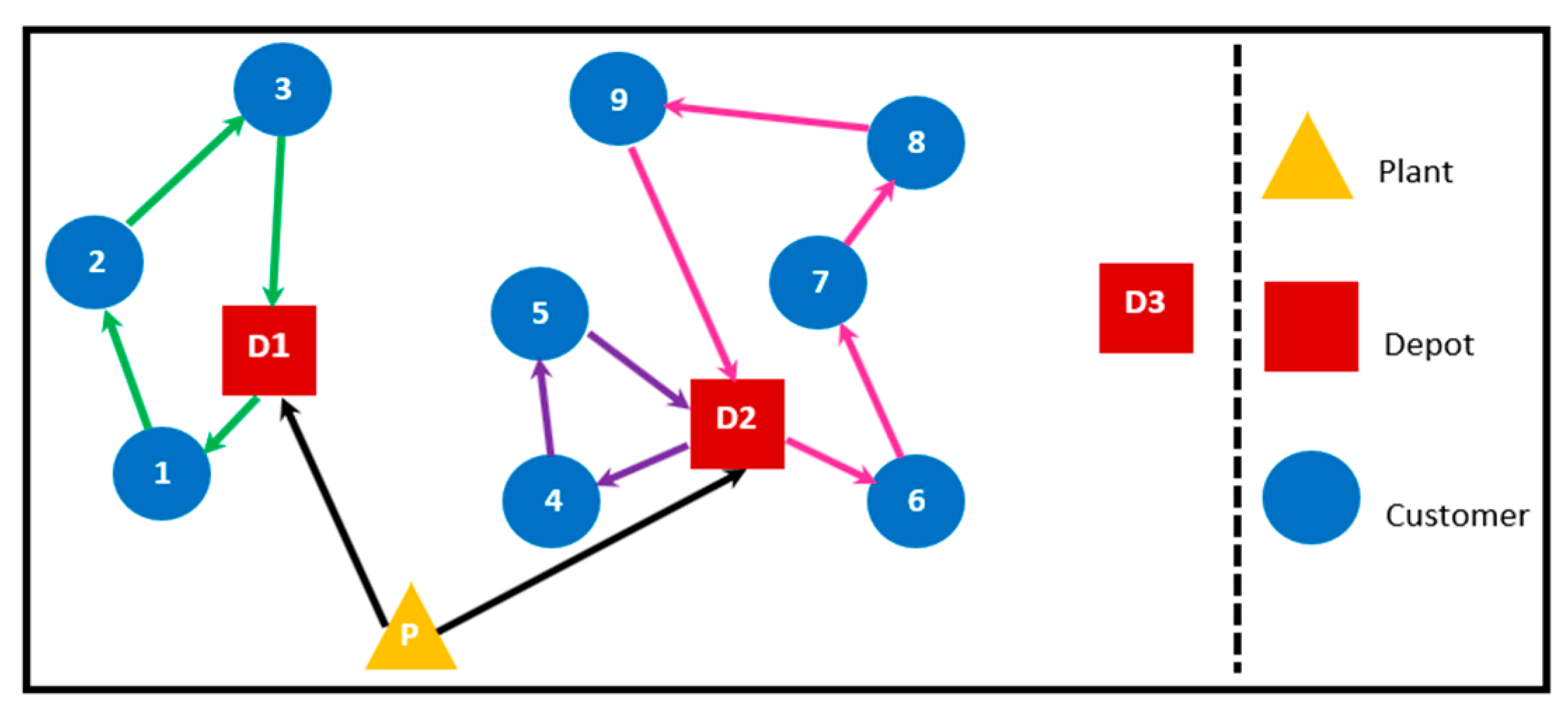
Given a set of the potential depots with fixed locations and customers with known demands and returns, the LIRP with EPQ model in reverse logistics is designed to determine the optimal location and number of open depots, the production quantity produced at each open depot as well as the routing of the assigned customers with known demands and returns to the open depots. The depots will function as a distributor as well as a collector. At the depot, the condition of the returned products will be inspected and classified into two categories: defect and non-defect items. The production setup cost will be affected where the non-defect items re-enters into the market, while the defect items will need to be counted in the process of production planning. The objective of the LIRP is to minimize the cost of establishing facilities, cost of inventory including production setup and holding, and cost of distance travelled by vehicles. Figure 1 shows an example of LIRP in the supply chain with three depots and nine customers. It can be seen from Figure 1 that customers 1, 2, and 3 are served by depot 1, while the remaining 6 customers are served by depot 2 using two vehicles. Depot 3 remains closed.
The mathematical formulation of LIRP with the EPQ model is given as follows. The objective and constraints are given below:
Sets:
  • I = set of all depots ( i   =   1 ,   2 ,     ,     I ) .
  • J = set of all customers ( j   =   1 ,   2 ,   ,     J ) .
  • K = set of all vehicles ( k   =   1 ,   2 ,     ,     K ) .
  • U = set of depots and customers ( u   =   1 ,   2 ,     ,     I + J ) .
Input Parameters:
  • D j = demand of customer j .
  • r j = non-defect items returned by customer j .
  • s j = defect items returned by customer j .
  • R j = returned products by customer j ( R j = r j + s j ).
  • d i j = distance from i to j .
  • V C k = capacity of vehicle k .
  • N = number of customers.
  • F i = fixed operating cost of depot i .
  • D C = distance cost per mile.
  • V D i = maximum through at the depot i .
  • K C = setup cost per production.
  • h = holding cost per unit inventory.
  • P = production rate.
  • T L i j k = total load of customer j at depot i by vehicle k .
Decision Variables:
  • z i   =   { 1 , if depot   i   is open 0 , otherwise   ,
  • y i j   =   { 1 , if depot   i   is assigned to customer   j 0 , otherwise ,
  • x i j k   =   { 1 , if arc   ( i , j )   is traveled by vehicle   k 0 , otherwise ,
  • Q i = optimal number of production quantity for each depot i ,
  • U l k = auxiliary variable for sub-tour elimination constraint in vehicle k of customer l .
min   z   =   i I F i z i + i U j U k K D C × d i j x i j k + K C i I j J [ ( D j r j + s j ) y i j Q i ] + h 2 P i I [ Q i ( P j J ( D j + r j + s j ) y i j ) ]  
subject to:
k K i U x i j k   =   1 ,   j J  
i I j J x i j k 1   ,   k K  
i U j J D j x i j k V C k   ,   k K  
i U j J ( r j + s j ) x i j k V C k ,   k K
T L i j k ( D j ( r j + s j ) ) x i j k V C k ,   i I ,   j J , k K
i U x i j k j U x j i k   =   0 ,   i I ,   k K  
j J D j y i j V D i z i ,   i I  
U l k U j k + N x l j k N 1 ,   l , j J , k K
l U x i l k + x u j k y i j 1 ,   i I ,   j J , k K  
y i j { 0 , 1 }   ,     i I ,   j J  
x i j k { 0 , 1 }   ,   i I ,   j J , k K  
z i { 0 , 1 }   ,   i I  
U l k 0   ,   l J , k K  
Q i 0   ,   i I .
The objective function of LIRP (Equation (1)) is to minimize the total fixed operating cost of depots, the total distance travelled cost by the vehicles, and the total cost of production setup and inventory holding. Constraints in Equations (2) and (3) indicate that each of the customers must be assigned in a single route and it can be served by only one vehicle. The total demands and total returns at each route cannot exceed the vehicle capacity limit and the total load on the vehicle at any arc must not exceed the vehicle capacity. These constraints are shown in Equations (4)–(6), respectively. Equation (7) states that the vehicle must start and end at the same depot. Besides the vehicle capacity limit, the capacity constraint for the depot is given in Equation (8). Equation (9) represents the new sub tour elimination constraint and Equation (10) specified that the customer will be assigned to the depot if there is a route from the depot. The binary values on the decision variable and the positive values for the auxiliary variable are defined in Equations (11)–(15), respectively.
Based on the objective function given in Equation (1), the total cost of inventory (TCI) consists of production setup cost and holding inventory cost. The optimal value of Q i can be obtained by deriving the first derivative of the cost function in Equation (16) with respect to Q i as follows:
TCI = Production setup cost + Inventory holding cost
T C I   =   K C i I j J [ ( D j r j + s j ) y i j Q i ] + h 2 P i I [ Q i ( P j J ( D j + r j + s j ) y i j ) ]   .
T C I Q i   =   K C i I j J [ ( D j r j + s j ) y i j Q i 2 ] + h 2 P i I [ ( P j J ( D j + r j + s j ) y i j ) ]   .
Let T C I Q i = 0, hence
K C i I j J [ ( D j r j + s j ) y i j Q i 2 ] + h 2 P i I [ ( P j J ( D j + r j + s j ) y i j ) ]   =   0   .
Q i   =   2 P ( K C ) i I j J ( D j r j + s j ) y i j h i I ( P j J ( D j + r j + s j ) y i j )   .  
The cost function of TCI is a convex function where the second derivative of the function is always non-negative (Equation (20)).
2 T C I Q i 2   =   K C i I j J [ ( D j r j + s j ) y i j Q i 3 ] 0   .  
From the objective function in Equation (1), we determine three decision planning as follows:
(1)
the number of open depots and assigned customers at each open depot.
(2)
the routing of vehicles delivering demands from the depot to the customers.
(3)
the optimal number of production quantity of each open depot.
We solve the problem iteratively where the allocation of customers to each depot has been assigned at the first stage with the possible number of open depots. At this stage, the vehicle capacity limit constraint has been relaxed. At the second stage, the process of minimizing location and routing with considering vehicle capacity constraint is done. To obtain the cost of inventory as stated in the objective function, the Q i is calculated by the Equation (19) where the formulation is depending on the decision variable of y i j and the total demand and returned from each customer at each depot. In other words, the inventory cost will be calculated when the decision variable for location and routing are found throughout the process of improvisation at each iteration. The process of minimizing the overall cost depends on the total operating depots, delivery routing, and inventory planning.

4. Hybrid Harmony Search-Simulated Annealing Algorithm

4.1. Harmony Search

Harmony Search (HS) is a population-based metaheuristic algorithm that mimics the music improvisation of a group orchestra. The musicians will improvise their harmonies with these three options: (1) select any pitch in the recorded harmony memory; (2) select and fix any previous pitch in memory; or (3) search a new music harmonisation within the range of the pitch. The process of obtaining the optimal solution is similar to this efficient search for a perfect state of harmony [32,33]. There are five main steps in the proposed HS:
  • Step 1: Initialisation
In HS, several solutions are generated to produce an initial population. The solutions can be generated either randomly or by the heuristics. A random initial population called harmony memory (HM) is created and sorted according to their fitness values. The number of solutions in the HM is the harmony memory size (HMS). An HM can be described in the following matrix:
H M     =   ( x 1 1 x 1 2 x 1 H M S x 2 1 x 2 2 x 2 H M S x n 1 x n 2 x n H M S | f ( x 1 ) f ( x 2 ) f ( x H M S ) )   ,
where,
  • x i j = decision variable of i   = 1 , 2 , , n and j   = 1 , 2 , , H M S ,
  • f ( x j ) = fitness function of x j for j   = 1 , 2 , , H M S .
  • Step 2: Parameter Setting
Harmony memory considering rate (HMCR) and pitch adjustment rate (PAR) are two main parameters used in the HS algorithm. An appropriate value of HMCR will lead to the choices of good solutions as an element of new solutions. The convergence will be slow if the value of HMCR is too high. Some potential good solutions will not be well explored. But if it is too low, only a few good solutions are selected for the next iteration. Therefore, to use memory effectively, the value of HMCR should be between 0.7 and 0.95 [34]. The speed of convergence in a standard HS algorithm may be slow if the value of PAR is too small. Besides, a high value of PAR is also not recommended. It can cause solutions to be stuck around a few potential optimal and easily get trapped in local optima. Due to this, [34] stated that the value of PAR is suggested to be between 0.1 and 0.5. However, this range may be suitable and valid for some problems only.
To balance the exploration and exploitation, instead of using a fixed value, in this paper, the proposed HS uses a dynamic value of H M C R i t and P A R i t introduced by [35]. The reason for reducing the H M C R i t slowly is to increase the probability of exploring more solution space, not in the HM. Hence, the global optimal can be attained [36]. The dynamic value of H M C R i t and P A R i t can avoid the solutions getting trapped in the local optimum quickly as well. With a slight modification, the proposed H M C R i t and P A R i t are reduced gradually when there is no improvement found in the solution. In this paper, the range values of [ H M C R m i n , H M C R m a x ] and [ P A R m i n , P A R m a x ] are set to be [0.7, 0.95] and [0.3, 0.9], respectively. Equations (23) and (24) below are the formulation of dynamic H M C R i t and P A R i t :
H M C R i t   =   H M C R m a x ( H M C R m a x H M C R m i n ) × i t M a x I t
P A R i t   =   P A R m a x ( P A R m a x P A R m i n ) × i t M a x I t   ,  
where,
  • i t = current iteration,
  • M a x I t = maximum number of iterations,
  • H M C R m a x = maximum value of HMCR,
  • H M C R m i n = minimum value of HMCR,
  • P A R m a x = maximum value of PAR,
  • P A R m i n = minimum value of PAR.
  • Step 3: Improvisation
In the proposed HS, to increase the speed of convergence, multi solutions are generated at each iteration and called HMnew. Each newly generated solution is taken from the HM randomly with the probability of HMCR, otherwise, it will be generated randomly within the range of the harmony vector. To further enhance the intensification of the method, the proposed HS implements the local optimization in three different ways: within a depot, between two depots, and within the vehicle route. Hence, five multi-neighbourhood local search techniques are proposed:
(1)
Swap: exchange the position of two random customers within the same route or between two different routes. Swapping can be done within a depot or between the depots.
(2)
Insertion: insert a customer in between two other random customers within the same depot.
(3)
Relocation: relocate the customers from the current depot to a new depot.
(4)
2-Opt: swapping two customers in the same vehicle route and reverse the substring between the swapped customers.
(5)
3-Opt: deleting three edges of the customers in the same vehicle route and create another three sub tours in three possible ways: non-reversing substring, with one reversing substring, or with two reversing substring.
The local optimization is applied to the new solution with the probability of P A R i t and the choice of multi-neighbourhood local search technique is randomly selected with equal probability. As mentioned earlier, we extended the methodology in [6] by adding two popular local search methods: 2-opt and 3-opt, as the local optimization techniques. The examples of these five techniques are graphically shown in Figure 2a–f.
  • Step 4: Update HM
To update the solutions in HM, the HMnew created at each iteration is combined with current HM. The solutions are sorted according to the value of the objective function. The best solutions with the size of HMS will be kept for the next iteration.
  • Step 5: Termination
Repeat Step 3 and 4. The proposed algorithm will be terminated when either the M a x I t is reached or t consecutive non-improving iterations are performed.

4.2. Hybrid Harmony Search—Simulated Annealing

To prevent the possibility of the HM population been trapped into local optima due to premature convergency, the proposed HS algorithm is further enhanced by hybridizing a SA with the implementation of probabilistic acceptance rule based on the Boltzmann factor, e Δ T i t during the improvisation procedure of the HS. In SA, the worst solution will be accepted within a probability and allows the search to proceed to its neighbourhood (Algorithm 1). By preserving the worst solution in a population, it provides practical randomness into the search to avoid the local extreme points. The probability of acceptance in SA is depending on the value of annealing temperature and the difference in the value of an objective function. At each iteration, the annealing temperature will be reduced according to the value of the cooling rate, which is a function of temperature. The higher value in the cooling rate, the slower the temperature reduction [37]. The procedures of probabilistic acceptance rule in SA described in Algorithm 1 are of a standard SA that has been adapted into the proposed hybrid HS-SA as shown in Algorithm 2.
Algorithm 1. SA Algorithm.
1: initialize parameter, T 0 = initial temperature, α = cooling rate;
2: generate initial solution, x ;
3: calculate objective function, f ( x ) ;
4: i t   =   0 ;
5: while ( i t < M a x I t )
6:  generate new solution x in the neighbourhood of x
7:  if f ( x ) < f ( x )
8:     x x
9:  else
10:     Δ   =   f ( x ) f ( x )
11:    if r a n d < e x p ( Δ T i t )
12:      x x
14:     T i t + 1   =   α × T i t
16:   i t   =   i t + 1
17: end while
Algorithm 2. Hybrid HS-SA Algorithm.
1: begin
2: define the parameter setting: H M C R m a x ,     H M C R m i n ,     P A R m a x ,     P A R m i n ,     H M S ,     T 0 ,     α ,     M a x I t ,     t
3: generate solution vectors and calculate fitness function for the initial population of HM.
4: while ( ( i t < M a x I t )   OR   ( n o n _ i m p r o v i n g   < t ) ) do
5:  while (no. of harmony vectors < HMnew) do
6:    do location-allocation and route allocation
7:    calculate H M C R i t and P A R i t
8:    if r a n d < H M C R i t
9:     select solution vectors from the HM randomly
10:     if r a n d < P A R i t
11:      implement one of the multi-neighbourhood search techniques randomly to create new neighbourhood solution, x
12:      if f ( x ) < f ( x )
13:        x x
14:      else
15:        Δ = f ( x ) f ( x )
16:       if r a n d < e x p ( Δ T i t )
17:         x x
19:        T i t + 1   = α × T i t
22:    else
23:     generate the new solution from the vector harmony space.
25:    do inventory planning
26:    update HM: sort and combine HM and HMnew
27:  end while
28:  update the best solution vectors of HM
29: end while
30: return the best solution

5. Computational Experiments and Discussion

In this section, computational experiments are performed to illustrate the performance of the proposed hybrid HS-SA compared with other approaches in the literature. The proposed algorithm is coded in MATLAB software R2017b on a laptop computer with 1.60 GHz Intel® Core™ i5-4200U CPU with 8 GB of RAM. The parameters configuration of the proposed algorithm is provided in Table 1. The test problem instances are three popular benchmark datasets of Perl, Gaskell, and Christofides with additional simulated data of returned products and production rate. The additional data were generated randomly by using a uniform distribution. The production rate is set to be greater than the total demand and returns, P > j J D j + r j + s j while the returned products, R j are generated by the uniform distribution of R j ~ U ( 0 , D j ) . We set 70% of the returned products as the non-defects ( r j ) items while the remaining are the defect items ( s j ). The characteristics of the dataset are given in Table 2.
To solve the LIRP problem, the location and allocation of the depots and customers are solved first. In the location-allocation problem, each of the customers is initially assigned to the nearest depots based on the Euclidean distance formulation. The customers will be moved around to the possible depots during the process of improvisation. The vehicle capacity limit constraint has been relaxed to minimize the number of open depots and it is assumed that only one vehicle is being used at each depot. However, the depot capacity limit should not be violated during the process. Then, the allocation of customers at each depot needs to be sequenced and divided into vehicles according to the vehicle capacity limit. This process is performed among the open depots only. The process of local optimization is performed within the open depots. Both depot capacity limits and vehicle capacity limits should not be violated. Finally, the inventory part is included during the process of minimizing the cost.
Since there is no study on the LIRP that utilizes the EPQ model for defect and non-defect items in reverse logistics from the literature, in order to validate the performance of the proposed hybrid HS-SA algorithm, the LRP will be solved first and compared with other heuristics and metaheuristics found in the literature that used the same benchmark datasets. Table 3, Table 4 and Table 5 present the comparative results of the three benchmark datasets on the proposed hybrid HS-SA with the heuristic method (HR) of [8], simulated annealing in [9] (SA-W) and [10] (SA-Z), hybrid tabu search and ant colony (TACO) from [11], particle swarm optimization (PSO) with different variants of particle swarm optimization which are: standard PSO, PSO with MPNS-GRASP (PMG), PSO with MPNS-GRASP and ENS (PMGE) and hybrid PSO (HLRP) in [12] and honey bee mating optimization (HBMO) in [13]. A standard HS (SHS) and the proposed HS (PHS) from [
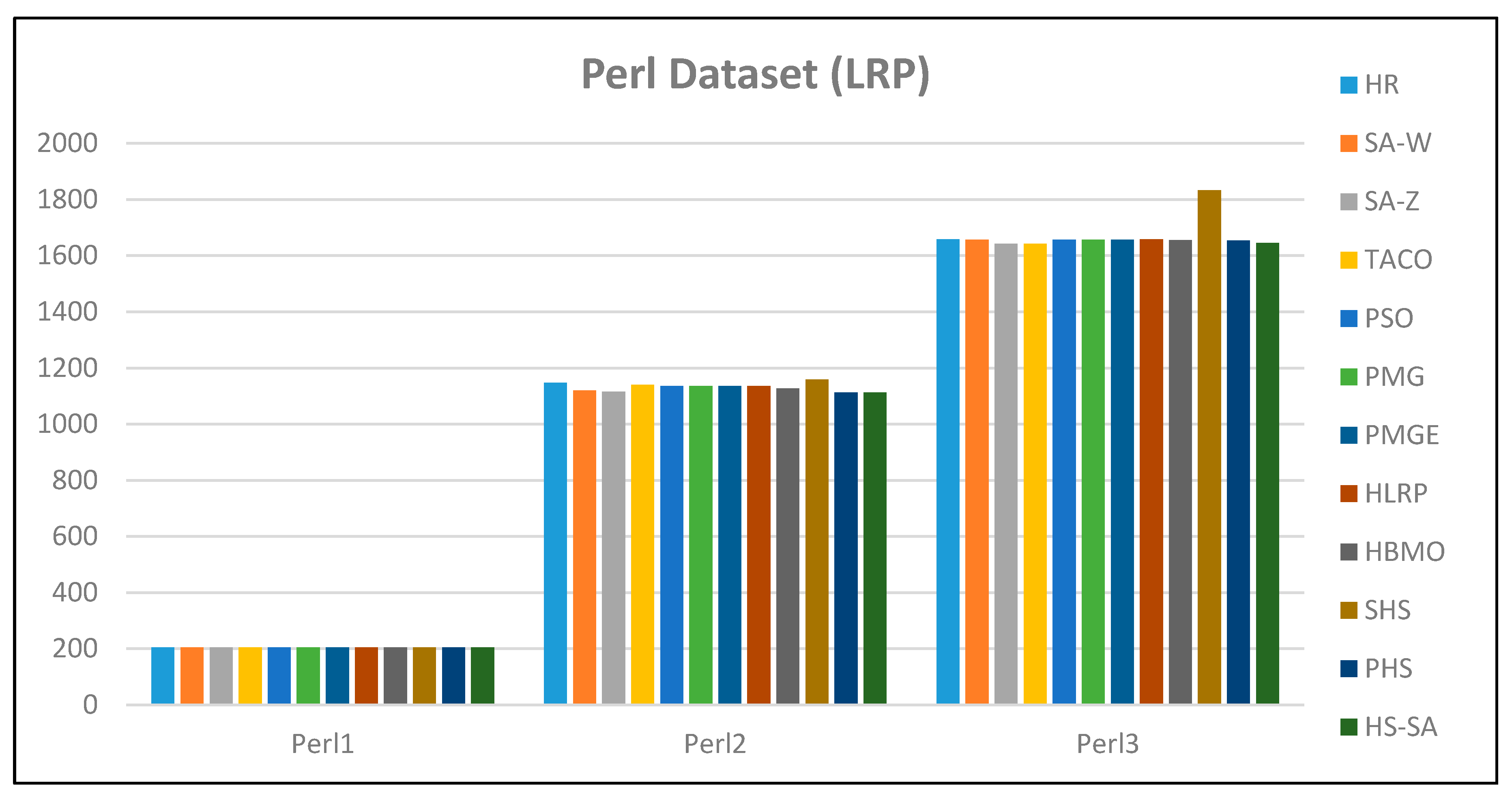
7] are also included for comparison in all experiments. For each problem instances, the proposed algorithm as well as SHS and PHS are performed for 10 independent runs. In each table, note that the numerical results of the selected algorithms are extracted from the original papers found in the literature and the best result of each problem instances is highlighted in bold.
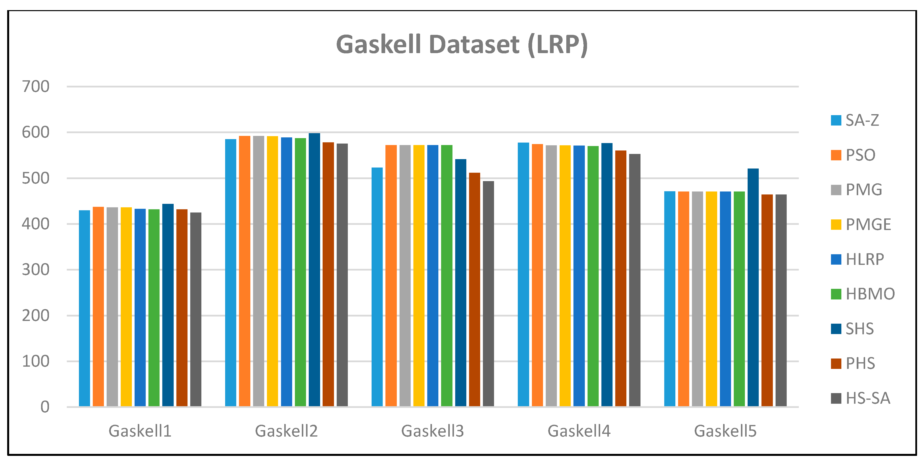
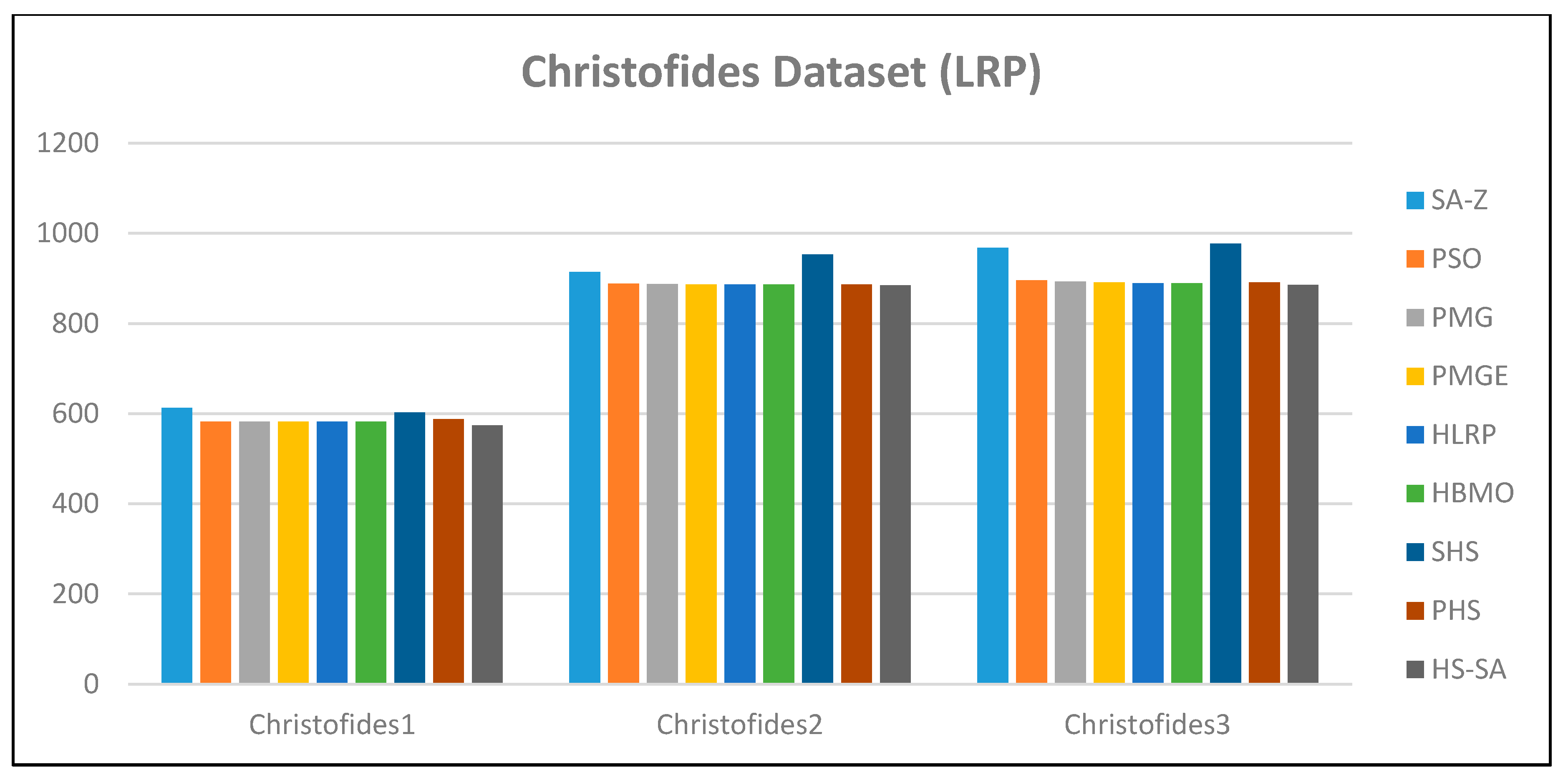
 Figure 3, Figure 4 and Figure 5 illustrate the results of Table 3, Table 4 and Table 5 in a bar chart respectively.
As compared to the SHS and PHS in [7], the hybrid HS-SA performed significantly better for all instances in Perl, Gaskell, and Christofides, except Perl 1. However, for Perl 3, results in SA-Z [10] and TACO [11] are slightly better than the hybrid HS-SA algorithm. All algorithms managed to find the optimal solution in Perl 1 since the number of customers and depots are small. The SHS did not perform well for medium and large size. This indicates that the SHS should be improved and modified to get better solutions [7]. From the numerical experiments in LRP, hybrid HS-SA has successfully solved the problem with comparable results. Therefore, the proposed algorithm will be used to solve the LIRP that utilizes the EPQ model for defect and non-defect items in reverse logistics.
The computational results for all test instances in LIRP are shown in Table 6, Table 7 and Table 8. Since there is no benchmark for the EPQ model in LIRP, the comparison is assessed between the hybrid HS-SA algorithm with SHS and PHS only. All algorithms are performed for 10 independent runs and the mean, standard deviation, coefficient of variation (C.V.), and the best result of each algorithm are reported in column 3–6 respectively. The Wilcoxon signed-rank test with α   =   0.05 is performed to test the significance of the results. As the Wilcoxon signed-rank test does not assume normality in the data, it can be used when this assumption has been violated and the use of the dependent t-test is inappropriate. The p-value of the test is reported in the last column of the tables. The best result of each problem instances is highlighted in bold. In addition, the best result of the all problem instances are summarized as a bar chart in Figure 6.
The Wilcoxon signed-rank test elicits a statistical significant difference in the performance of finding the minimum cost of the LIRP between the hybrid HS-SA and the SHS and PHS across all the datasets (p-value < 0.005) based on the difference in the median cost. These tests are used to show that the results are significant, supporting that the proposed algorithm will produce results that are different from the results of the SHS and PHS. Apart from the Perl 1 instance where the proposed algorithm produced the same results as SHS and PHS, all other datasets showed p-values of less than 0.05. This means the results generated by the hybrid HS-SA is significant and different from the values from the SHA and PHS. So, the results from the proposed algorithm is significant from the other works, but is it better? From Table 6, Table 7 and Table 8, the hybrid HS-SA outperforms the solutions in SHS and PHS for all cases of datasets of Perl, Gaskell, and Christofides. For this, we use the C.V. values. The lower the value of the C.V., the more precise the estimate. As reported in Table 6, Table 7 and Table 8, all the C.V. values are low which supports the high predictiveness of the proposed algorithm.
Table 9, Table 10 and 
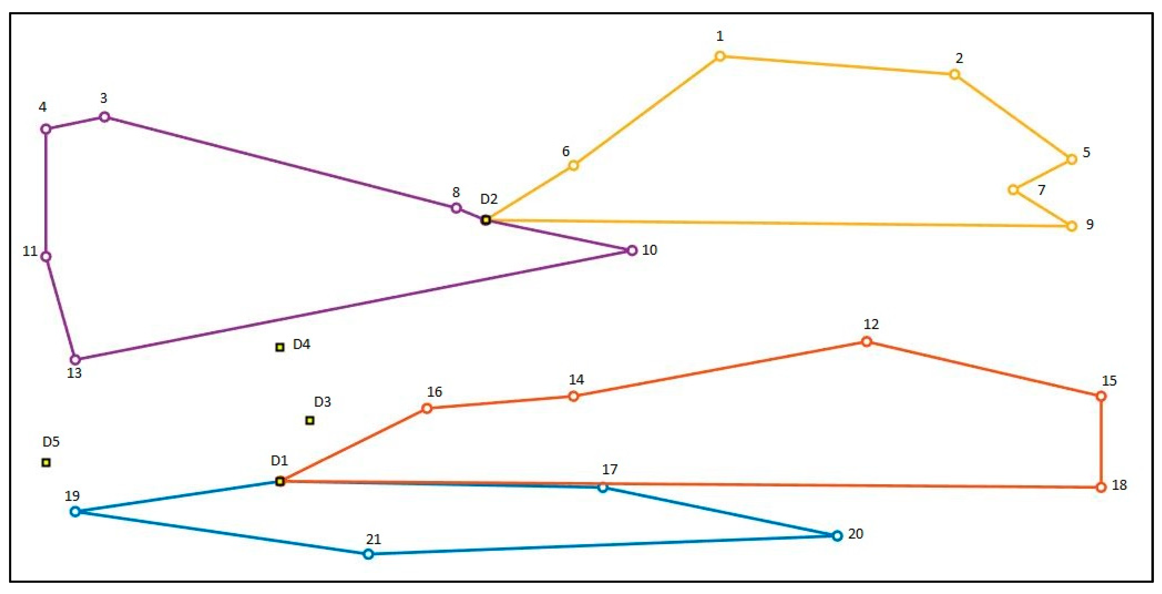
Table 11 present the detailed results of all problem instances produced by the proposed hybrid HS-SA for LIRP. The total cost for each problem instance is highlighted in bold. These tables served as the benchmark for the LIRP. For instance, Gaskell 1 required two depots with a fixed cost of 50 each to serve all the 21 customers with four vehicles (see, Table 10). In depot 1, with the inventory cost of 573.05, two vehicles are deployed to serve the customers (19→21→20→17) and (18→15→12→14→16) with costs of 59.45 and 86.90 respectively. While in depot 2, with the inventory cost of 577.74, two vehicles are used to serve the customers (9→7→5→2→1→6) and (8→3→4→11→13→10) with costs of 83.01 and 95.55 respectively. In this result, the best solution obtained suggest to close Depot 3–5. The overall minimum cost for Gaskell 1 is 1575.7. Figure 7 illustrate the topological layout of the Gaskell 1 produced by the proposed hybrid HS-SA for LIRP.

6. Conclusions and Future Work

The integration of facility location, inventory planning, and vehicle routing is one of the most challenging problems in the supply chain network design. In this study, the Economic Production Quantity (EPQ) model of reverse logistics that considers the returned products from the customers is included during the process of optimization. Since the problem is NP-hard, a hybrid population-based metaheuristic called hybrid Harmony Search-Simulated Annealing (HS-SA) algorithm is proposed. Computational experiments on three sets of popular benchmark instances show that the proposed hybrid HS-SA algorithm is successful in finding better solutions as compared to a standard HS, as well as other approaches from the literature of Location-Routing Problem (LRP) and Location-Inventory-Routing Problem (LIRP). For future work, the HS can be hybridized with other metaheuristic methods such as differential evolution, genetic algorithm, and tabu search to further enhanced the efficiency of the approach. Environmental issues such as the CO2 emission and the use of electric vehicles can also be integrated into the model to be solved.

Author Contributions

Conceptualization, F.M. and L.S.L.; methodology, F.M. and L.S.L.; software, F.M.; validation, F.M., L.S.L., and H.-V.S.; formal analysis, F.M., L.S.L., and H.-V.S.; investigation, F.M. and L.S.L.; writing—original draft preparation, F.M. and L.S.L.; writing—review and editing, F.M., L.S.L., and H.-V.S.; supervision, L.S.L. All authors have read and agreed to the published version of the manuscript.

Funding

This research was supported by Universiti Putra Malaysia (UPM) through Geran Putra-Inisiatif Putra Siswazah (GP-IPS/2017/9579400).

Conflicts of Interest

The authors declare no conflict of interest.

References

  1. Prahinski, C.; Kocabasoglu, C. Empirical research opportunities in reverse supply chains. Omega 2006, 34, 519–532. [Google Scholar] [CrossRef]
  2. Tibben-Lembke, R.S. The impact of reverse logistics on the total cost of ownership. J. Mark. Theory Pract. 1998, 6, 51–60. [Google Scholar] [CrossRef]
  3. Guide, V.D.R., Jr.; Souza, G.C.; Van Wassenhove, L.N.; Blackburn, J.D. Time value of commercial product returns. Manag. Sci. 2006, 52, 1200–1214. [Google Scholar] [CrossRef] [Green Version]
  4. Daugherty, P.J.; Richey, R.G.; Genchev, S.E.; Chen, H. Reverse logistics: Superior performance through focused resource commitments to information technology. Transp. Res. Part E Logist. Transp. Rev. 2005, 41, 77–92. [Google Scholar] [CrossRef]
  5. Petersen, J.A.; Kumar, V. Perceived risk, product returns, and optimal resource allocation: Evidence from a field experiment. J. Mark. Res. 2015, 52, 268–285. [Google Scholar] [CrossRef] [Green Version]
  6. Misni, F.; Lee, L.S. Harmony search for multi-depot vehicle routing problem. Malays. J. Math. Sci. 2019, 13, 311–328. [Google Scholar]
  7. Misni, F.; Lee, L.S. Harmony search algorithm for location-routing problem in supply chain network design. ASM Sci. J. 2019, 12, 48–56. [Google Scholar]
  8. Perl, J.; Daskin, M.S. A warehouse location-routing problem. Transp. Res. Part B Methodol. 1985, 19, 381–396. [Google Scholar] [CrossRef]
  9. Wu, T.H.; Low, C.; Bai, J.W. Heuristic solutions to multi-depot location-routing problems. Comput. Oper. Res. 2002, 29, 1393–1415. [Google Scholar] [CrossRef]
  10. Zhang, Y.; Qi, M.; Lin, W.H.; Miao, L. A metaheuristic approach to the reliable location routing problem under disruptions. Transp. Res. Part E Logist. Transp. Rev. 2015, 83, 90–110. [Google Scholar] [CrossRef]
  11. Wang, X.; Sun, X.; Fang, Y. A two-phase hybrid heuristic search approach to the location-routing problem. In Proceedings of the 2005 IEEE International Conference on Systems, Man and Cybernetics, Waikoloa, HI, USA, 12 October 2005; Volume 4, pp. 3338–3343. [Google Scholar]
  12. Marinakis, Y.; Marinaki, M. A particle swarm optimization algorithm with path relinking for the location routing problem. J. Math. Model. Algorithms 2008, 7, 59–78. [Google Scholar] [CrossRef]
  13. Marinakis, Y.; Marinaki, M.; Matsatsinis, N. Honey bees mating optimization for the location routing problem. In Proceedings of the 2008 IEEE International Engineering Management Conference, Estoril, Portugal, 28–30 June 2008; pp. 1–5. [Google Scholar]
  14. Alaei, S.; Setak, M. Multi objective coordination of a supply chain with routing and service level consideration. Int. J. Prod. Econ. 2015, 167, 271–281. [Google Scholar] [CrossRef]
  15. Cheng, C.; Yang, P.; Qi, M.; Rousseau, L.M. Modeling a green inventory routing problem with a heterogeneous fleet. Transp. Res. Part E Logist. Transp. Rev. 2017, 97, 97–112. [Google Scholar] [CrossRef]
  16. Soysal, M.; Bloemhof-Ruwaard, J.M.; Haijema, R.; van der Vorst, J.G. Modeling a green inventory routing problem for perishable products with horizontal collaboration. Comput. Oper. Res. 2018, 89, 168–182. [Google Scholar] [CrossRef]
  17. Rahimi, M.; Baboli, A.; Rekik, Y. Sustainable inventory routing problem for perishable products by considering reverse logistic. IFAC Pap. Online 2016, 49, 949–954. [Google Scholar] [CrossRef]
  18. Lei, L.; Liu, S.; Ruszczynski, A.; Park, S. On the integrated production, inventory, and distribution routing problem. IIE Trans. 2006, 38, 955–970. [Google Scholar] [CrossRef] [Green Version]
  19. Bard, J.F.; Nananukul, N. Heuristics for a multiperiod inventory routing problem with production decisions. Comput. Ind. Eng. 2009, 57, 713–723. [Google Scholar] [CrossRef]
  20. Dai, Z.; Aqlan, F.; Zheng, X.; Gao, K. A location-inventory supply chain network model using two heuristic algorithms for perishable products with fuzzy constraints. Comput. Ind. Eng. 2018, 119, 338–352. [Google Scholar] [CrossRef]
  21. Liao, S.H.; Hsieh, C.L.; Lai, P.J. An evolutionary approach for multi-objective optimization of the integrated location–inventory distribution network problem in vendor-managed inventory. Expert Syst. Appl. 2011, 38, 6768–6776. [Google Scholar] [CrossRef]
  22. Asl-Najafi, J.; Zahiri, B.; Bozorgi-Amiri, A.; Taheri-Moghaddam, A. A dynamic closed-loop location-inventory problem under disruption risk. Comput. Ind. Eng. 2015, 90, 414–428. [Google Scholar] [CrossRef]
  23. Wang, Z.; Yao, D.Q.; Huang, P. A new location-inventory policy with reverse logistics applied to B2C e-markets of China. Int. J. Prod. Econ. 2007, 107, 350–363. [Google Scholar] [CrossRef]
  24. Tancrez, J.S.; Lange, J.C.; Semal, P. A location-inventory model for large three-level supply chains. Transp. Res. Part E Logist. Transp. Rev. 2012, 48, 485–502. [Google Scholar] [CrossRef] [Green Version]
  25. Puga, M.S.; Tancrez, J.S. A heuristic algorithm for solving large location–inventory problems with demand uncertainty. Eur. J. Oper. Res. 2017, 259, 413–423. [Google Scholar] [CrossRef]
  26. Diabat, A.; Abdallah, T.; Henschel, A. A closed-loop location-inventory problem with spare parts consideration. Comput. Oper. Res. 2015, 54, 245–256. [Google Scholar] [CrossRef]
  27. Diabat, A.; Theodorou, E. A location–inventory supply chain problem: Reformulation and piecewise linearization. Comput. Ind. Eng. 2015, 90, 381–389. [Google Scholar] [CrossRef]
  28. Li, Y.; Guo, H.; Wang, L.; Fu, J. A hybrid genetic-simulated annealing algorithm for the location-inventory-routing problem considering returns under E-supply chain environment. Sci. World J. 2013, 2013, 125893. [Google Scholar] [CrossRef]
  29. Liu, B.; Chen, H.; Li, Y.; Liu, X. A pseudo-parallel genetic algorithm integrating simulated annealing for stochastic location-inventory-routing problem with consideration of returns in e-commerce. Discret. Dyn. Nat. Soc. 2015, 2015, 586581. [Google Scholar] [CrossRef]
  30. Deng, S.; Li, Y.; Guo, H.; Liu, B. Solving a closed-loop location-inventory-routing problem with mixed quality defects returns in e-commerce by hybrid ant colony optimization algorithm. Discret. Dyn. Nat. Soc. 2016, 2016, 6467812. [Google Scholar] [CrossRef] [Green Version]
  31. Yuchi, Q.; He, Z.; Yang, Z.; Wang, N. A location-inventory-routing problem in forward and reverse logistics network design. Discret. Dyn. Nat. Soc. 2016, 2016, 3475369. [Google Scholar] [CrossRef] [Green Version]
  32. Geem, Z.W.; Kim, J.H.; Loganathan, G.V. A new heuristic optimization algorithm: Harmony search. Simulation 2001, 76, 60–68. [Google Scholar] [CrossRef]
  33. Lee, K.S.; Geem, Z.W. A new meta-heuristic algorithm for continuous engineering optimization: Harmony search theory and practice. Comput. Methods Appl. Mech. Eng. 2005, 194, 3902–3933. [Google Scholar] [CrossRef]
  34. Yang, X.S. Harmony Search as a Metaheuristic Algorithm. In Music-Inspired Harmony Search Algorithm: Theory and Applications; Geem, Z.W., Ed.; Studies in Computational Intelligence; Springer: Berlin/Heidelberg, Germany, 2009; Volume 191, pp. 1–14. [Google Scholar]
  35. Mahdavi, M.; Fesanghary, M.; Damangir, E. An improved harmony search algorithm for solving optimization problems. Appl. Math. Comput. 2007, 188, 1567–1579. [Google Scholar] [CrossRef]
  36. Moh’d Alia, O.; Mandava, R. The variants of the harmony search algorithm: An overview. Artif. Intell. Rev. 2011, 36, 49–68. [Google Scholar] [CrossRef]
  37. Kirkpatrick, S.; Gelatt, C.D.; Vecchi, M.P. Optimization by simulated annealing. Science 1983, 220, 671–680. [Google Scholar] [CrossRef]
Figure 1. Example of a LIRP with 3 depots and 9 customers.
Applsci 10 06625 g001
Figure 2. The figures show how each of the multi-neighbourhood search techniques finds their neighborhood: (a) Swap within depot: customer 1 and 2 are swapped within the same depot; (b) Insertion: customer 3 are inserted in between depot and customer 1 in the route sequence; (c) Swap between depots: customer 6 in depot 1 is swapped with customer 1 in depot 2; (d) Relocation: customer 6 in depot 2 is moved to depot 1; (e) 2–Opt: swap customer 1 and 4 in the same route and the route sequence between swapped customers are reversed; (f) 3-Opt: three possibilities of 3-Opt which are either non-reversing, one reversing or two reversing substring.
Applsci 10 06625 g002
Figure 3. Best result of Perl dataset for LRP.
Applsci 10 06625 g003
Figure 4. Best result of Gaskell dataset for LRP.
Applsci 10 06625 g004
Figure 5. Best result of Christofides dataset for LRP.
Applsci 10 06625 g005
Figure 6. Best result of Perl, Gaskell, and Christofides dataset in LIRP for SHS, PHS, and HS-SA.
Applsci 10 06625 g006
Figure 7. Topological layout of the Gaskell 1 produced by HS-SA for LIRP.
Applsci 10 06625 g007
Table 1. Parameters Setting for SHS, PHS, and HS-SA.
ParameterSHSPHSHS-SA
HMS300300300
HMCR0.85 [ 0.7 , 0.95 ] [ 0.7 , 0.95 ]
PAR0.55 [ 0.3 , 0.9 ] [ 0.3 , 0.9 ]
M a x I t 10,00050005000
t 500100100
T 0 30
α 0.98
Table 2. Characteristics of Perl, Gaskell, and Christofides dataset.
No. of DepotNo. of CustomerDepot CapacityVehicle Capacity
Perl 1212280140
Perl 21555550120
Perl 3785850160
Gaskell 152115,0006000
Gaskell 252215,0004500
Gaskell 352915,0004500
Gaskell 453235,0008000
Gaskell 553615,000250
Christofides 155010,000160
Christofides 2107510,000140
Christofides 31010010,000200
Table 3. Comparative results of Perl dataset for LRP.
AlgorithmPerl 1Perl 2Perl 3
MeanBestMeanBestMeanBest
HR204.01146.91657.6
SA-W204.01119.81656.7
SA-Z204.01115.41642.0
TACO204.01139.91642.6
PSO204.01135.91656.9
PMG204.01136.21656.9
PMGE204.01135.91656.9
HLRP204.01135.91657.1
HBMO204.01127.11655.2
SHS204.0204.01161.41158.81846.31832.1
PHS204.0204.01115.61113.21666.01653.0
HS-SA204.0204.01114.71113.21658.41645.0
Table 4. Comparative results of Gaskell dataset for LRP.
AlgorithmGaskell 1Gaskell 2Gaskell 3Gaskell 4Gaskell 5
MeanBestMeanBestMeanBestMeanBestMeanBest
SA-Z429.6585.1523.2577.6471.3
PSO437.1592.1572.1574.1470.7
PMG435.9591.8572.1571.7470.7
PMGE435.9591.7572.1571.7470.7
HLRP432.9588.5572.1570.8470.7
HBMO431.9587.2572.1569.8470.7
SHS449.1443.7602.9598.0550.6541.2578.7576.2528.5520.7
PHS437.9431.7584.3577.9522.7511.8562.6559.9475.5464.1
HS-SA429.3424.9577.3575.2502.5493.1559.5552.4473.5464.1
Table 5. Comparative results of Christofides dataset for LRP.
AlgorithmChristofides 1Christofides 2Christofides 3
MeanBestMeanBestMeanBest
SA-Z612.6914.0967.6
PSO582.7888.9895.7
PMG582.7887.1893.2
PMGE582.7886.9891.5
HLRP582.7886.3889.4
HBMO582.7886.3889.4
SHS606.0602.9961.2953.3981.6977.6
PHS591.2587.7889.3886.7894.6891.6
HS-SA577.8573.6888.2885.0891.9885.5
Table 6. Comparative results of Perl dataset in LIRP for SHS, PHS, and HS-SA.
InstanceAlgorithmMeanStd. Dev.C.V.Bestp-Value
SHS263.275.99 × 10−142.28 × 10−16263.31.000
Perl 1PHS263.275.99 × 10−142.28 × 10−16263.31.000
HS-SA263.275.99 × 10−142.28 × 10−16263.3
SHS1693.183.26460.00191689.50.005
Perl 2PHS1646.252.11410.00131643.90.005
HS-SA1485.271.93090.00131482.4
SHS2271.268.90400.00392257.70.005
Perl 3PHS2099.915.50060.00262096.20.005
HS-SA2082.904.50940.00222078.0
Table 7. Comparative results of Gaskell dataset in LIRP for SHS, PHS, and HS-SA.
InstanceAlgorithmMeanStd. Dev.C.V.Bestp-Value
SHS1592.137.14440.00451586.20.005
Gaskell 1PHS1585.234.99270.00311578.50.028
HS-SA1579.263.74380.00241575.7
SHS1042.763.72710.00361039.00.005
Gaskell 2PHS1009.801.94080.00191008.90.022
HS-SA1007.321.83960.00181006.1
SHS829.585.96080.0072820.20.005
Gaskell 3PHS797.705.62140.0070790.30.013
HS-SA789.515.22950.0066780.9
SHS1032.743.30670.00321030.60.005
Gaskell 4PHS1021.372.65790.00261018.10.028
HS-SA1018.491.59200.00161017.0
SHS610.806.46250.0106604.70.005
Gaskell 5PHS602.503.93020.0065599.20.005
HS-SA571.793.63030.0063566.9
Table 8. Comparative results of Gaskell dataset in LIRP for SHS, PHS, and HS-SA.
InstanceAlgorithmMeanStd. Dev.C.V.Bestp-Value
SHS848.402.89830.0034845.40.005
Christofides 1PHS834.992.43240.0029833.60.005
HS-SA819.762.23420.0027817.9
SHS1220.874.48230.00371214.30.005
Christofides 2PHS1151.872.35610.00201148.20.007
HS-SA1149.482.28280.00201146.1
SHS1384.603.23450.00231381.00.005
Christofides 3PHS1349.852.97440.00221347.20.005
HS-SA1312.492.69490.00201307.2
Table 9. Distribution of routes and costs for Perl dataset generated by HS-SA for LIRP.
InstanceDepotVehicleRouteCost
DepotDistanceInventoryTotal
Perl 1D1V1D1→9→8→6→1→2→3→7→D110044.3459.36263.27
V2D1→10→12→11→5→4→D159.63
Perl 2D5V1D5→38→54→39→55→43→34→D524048.85123.901482.43
V2D5→23→28→12→17→22→30→D547.56
V3D5→8→3→7→31→29→19→D528.78
V4D5→33→14→27→16→32→45→D552.26
D10V5D10→13→1→2→42→4→9→D1024018.45123.18
V6D10→6→10→21→51→37→47→D1056.42
V7D10→44→46→40→52→50→53→D1062.37
V8D10→5→11→D103.41
D12V9D12→36→35→24→26→18→15→D1224040.02122.15
V10D12→41→20→49→48→25→D1235.08
Perl 3D2V1D2→54→59→58→39→56→57→40→55→D237269.27171.632077.97
V2D2→62→61→65→66→68→69→27→16→D244.90
V3D2→22→17→28→75→23→29→19→30→D243.98
V4D2→63→14→70→71→12→73→74→72→D244.75
V5D2→32→38→2→45→33→D226.34
D4V6D4→4→42→15→31→7→3→8→5→D437237.06140.58
V7D4→44→64→80→52→46→43→34→1→D463.27
V8D4→47→53→50→81→83→67→82→11→D451.73
D6V9D6→49→76→51→79→13→78→21→20→D637253.65120.73
V10D6→24→37→77→10→60→9→6→41→D639.54
V11D6→25→36→85→18→84→26→35→48→D654.54
Table 10. Distribution of routes and costs for Gaskell dataset generated by HS-SA for LIRP.
InstanceDepotVehicleRouteCost
DepotDistanceInventoryTotal
Gaskell 1D1V1D1→19→21→20→17→D15059.45573.051575.70
V2D1→18→15→12→14→16→D186.90
D2V3D2→9→7→5→2→1→6→D25083.01577.74
V4D2→8→3→4→11→13→10→D295.55
Gaskell 2D1V1D1→9→D15041.23430.911006.14
V2D1→10→13→11→6→1→2→3→16→15→14→17→22→20→19→18→12→D1334.73
V3D1→7→8→5→4→21→D1149.27
Gaskell 3D3V1D3→2→D35042.76287.76780.87
V2D3→21→14→8→9→17→7→13→16→15→12→11→10→23→18→19→20→D3219.24
V3D3→22→26→28→27→29→25→24→6→1→5→4→3→D3181.11
Gaskell 4D3V1D3→26→27→16→28→29→D350111.77464.651017.0
V2D3→14→17→25→24→23→22→20→21→18→19→15→D3140.46
V3D3→11→5→6→7→8→9→10→32→13→1→D390.59
V4D3→31→12→2→4→3→30→D3159.53
Gaskell 5D5V1D5→22→28→29→30→36→35→34→33→27→D550108.88102.78566.93
V2D5→21→20→26→32→31→25→19→13→14→D5101.70
V3D5→15→9→8→7→1→2→3→4→10→D597.50
V4D5→16→17→11→5→6→12→18→24→23→D5106.07
Table 11. Distribution of routes and costs for Christofides dataset generated by HS-SA for LIRP.
InstanceDepotVehicleRouteCost
DepotDistanceInventoryTotal
Christofides 1D2V1D2→4→17→37→15→33→45→44→42→19→40→41→13→D240119.68130.14817.86
V2D2→6→48→23→7→43→24→14→25→D298.12
V3D2→18→46→27→32→11→38→5→12→47→D278.65
D5V4D5→1→8→26→31→28→3→36→35→20→22→D54095.21114.14
V5D5→2→16→50→9→49→10→39→30→34→21→29→D5101.92
Christofides 2D1V1D1→17→3→44→24→49→16→51→6→D14085.59143.311146.09
V2D1→8→35→14→11→53→7→D143.90
V3D1→32→50→18→55→25→9→40→D198.72
V4D1→19→59→66→65→38→10→58→D197.16
V5D1→4→27→52→46→34→67→D134.29
V6D1→30→48→74→28→62→73→63→33→2→68→75→D191.12
V7D1→54→13→57→15→5→29→45→D175.40
V8D1→26→72→31→39→12→D177.34
D5V9D5→69→71→60→70→20→37→36→D54061.19117.74
V10D5→61→64→42→41→56→23→43→1→22→21→ 47→D5140.33
Christofides 3D3V1D3→69→1→50→33→81→51→9→35→71→65→66→20→30→70→D340110.56154.431307.24
V2D3→88→62→19→11→64→49→36→47→46→8→82→48→7→52→D3127.18
V3D3→31→10→63→90→32→D351.83
D5V4D5→89→18→60→83→45→17→84→5→59→94→53→28→27→D54097.34136.43
V5D5→95→92→37→91→44→14→38→86→16→61→93→99→96→6→D592.79
V6D5→13→87→97→98→85→100→42→43→15→57→2→40→58→D595.14
D8V7D8→12→80→68→76→77→3→79→78→34→29→24→55→25→54→D84095.56130.85
V8D8→4→39→67→23→56→75→41→22→74→72→73→21→26→D895.13

