Article

Optimal Design and Control of a Two-Speed Planetary Gear Automatic Transmission for Electric Vehicle

School of Mechanical Engineering, Shanghai Jiao Tong University, Shanghai 200240, China
*
Author to whom correspondence should be addressed.
Appl. Sci. 2020, 10(18), 6612; https://doi.org/10.3390/app10186612
Submission received: 31 August 2020 / Revised: 15 September 2020 / Accepted: 19 September 2020 / Published: 22 September 2020

Abstract

:
Multispeed transmissions are helpful for improvement of the economy and drivability of electric vehicles (EVs). In this paper, we propose a two-speed transmission based on dual planetary gear mechanism, in which shifts are realized by torque transfer between two brakes located on ring gears. To synthesize the dynamic and economic performances of the vehicle, a multiobjective optimization problem is constructed for gear ratio optimization and Pareto-optimal solutions of gear ratio combinations are obtained by Nondominated sorting genetic algorithm-II (NSGA-II). In particular, the minimum electric energy consumption of the EV is calculated with a fast Dynamic Programming (DP) in each iteration. Following this, a constant-output-torque control (COTC) scheme is adopted for the torque phase and inertia phase of gearshift process to ensure constant output torque on the wheel. To enhance transient responses, the feedforward–feedback controller structure is applied and a disturbance observer is integrated to improve robustness. Simulation results demonstrate that the two-speed transmission has much better performance in terms of acceleration time and energy economy compared to the fixed-ratio transmission, and the proposed gearshift control method is able to achieve fast and smooth gear shift robustly while maintaining constant output torque.

1. Introduction

Electric vehicles (EVs) are promising alternatives to conventional vehicles that use fossil fuels [1]. Benefiting from the wide operating range of the electric motor and minimizing the cost, volume, and mass of the power train, most EVs in the market are equipped with fixed-ratio single reduction rather than multispeed transmission, e.g., Nissan Leaf, Renault ZOE, and Tesla Model 3. However, motor operating points may deviate from the high-efficiency region under actual driving conditions for daily use and the ratio of single reduction on EVs must be designed as a trade-off between dynamic and economic performances [2]. Researchers have proved benefits of using multispeed transmissions on EVs through simulations and experiments [3,4,5,6,7]. Integrating a multiple-speed transmission into EVs can make optimum use of high-efficiency motor operating ranges, which means that the motor and battery can be downsized compared to the baseline drivetrain configuration consisting of a single-speed transmission [3,4]. Reference [2] indicated that choosing a suitable two-speed transmission not only improves EVs’ dynamic performance with little additional initial manufacturing cost, but also saves customers’ money in the long term.
The application of a multispeed transmission for EVs consists of dual clutch transmission (DCT) [8,9], continuous variable transmission (CVT) [5], automatic transmission (AT) [10,11], and automated manual transmission (AMT) [6,11,12,13]. Each of the above transmission configurations has its own merits and demerits. The first three can achieve a seamless gearshift by clutch-to-clutch control, but this makes the control system complex and expensive. The AMT used in EVs has a simpler mechanical structure and lower cost, in which the gearshift is mainly achieved through active motor speed synchronization, while torque interruption is inevitable during the gearshift process.
Gear ratio optimization of the multispeed transmission is necessary in order to balance the dynamic and economic performance. In [2], the gear ratios of a two-speed DCT and a simplified CVT are designed according to target vehicle performance characteristics, i.e., top speed, max grade, and acceleration. The selection of the optimal gear ratio for the CVT-based two-speed system has been carried out via an optimization procedure which takes into account the efficiency characteristics of the whole vehicle power-train [14]. However, the above design optimizations are based on fixed drive cycle, which may not be necessarily optimal when applied to different drive cycle or to the entire driving profile of a vehicle [15]. Therefore, reference [6] designed a composite gear shifting schedule under the combined urban and suburban drive cycles in the optimization process. Researches on gearshift control of transmissions for EVs have also been observed. In [16], optimal control methods are used to fulfill the constant-output speed and constant-output torque shift control, with the actuator limits considered. This work is further improved by complementing with a backstepping controller which serves as the feedback component [17]. Hybrid Minimum Principle (HMP) is used to handle state jumps at the switching points of different stages in gearshift [10]. PID (Proportional-integral-derivative) controllers are applied in references [18,19]. Effects of the slip speed reference in the inertia phase are discussed in reference [20]. In [21], torque observers are adopted to facilitate shifting control of a two-speed transmission for EV.
Novel configurations and control strategies are brought about with the rapid development of EV. For high-performance models, intermittent power loss is unacceptable. In such cases, planetary-gear-based transmissions (PGTs) may be more promising candidates. In this paper, we propose a two-speed transmission based on dual planetary gear mechanism and introduce an integrated gearshift strategy using feedforward–feedback control with disturbance compensation, for both torque phase and inertia phase. The paper is organized as follows: Section 2 shows the power-train topology of the two-speed transmission. The gear ratio optimization based on Nondominated sorting genetic algorithm-II (NSGA-II) approach is applied in Section 3. Section 4 presents the development process of the constant-output-torque control (COTC) strategy for torque phase and inertia phase. At last, summary and conclusions are given in Section 5.

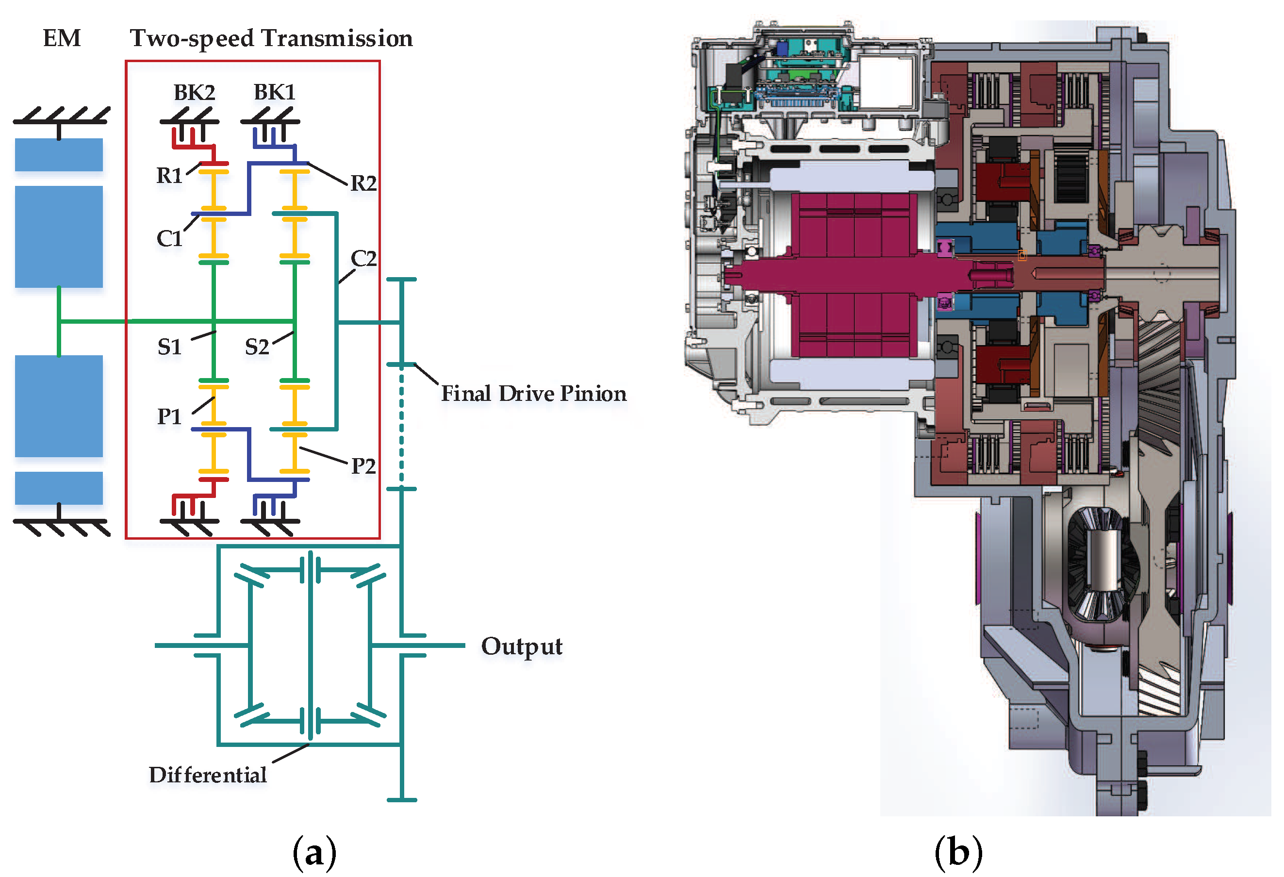
2. Topology Structure of The Drivetrain

The power-train topology of the EV adopting the proposed two-speed transmission is illustrated in Figure 1, including an electric motor, two-speed transmission, final drive, and differential. To be more specific, the two-speed transmission consists of dual planetary gear sets, where the input of the transmission is S1 mechanically connected to the output shaft of motor and C2 is regarded as the output of the transmission. Two planetary gear sets have up to four degrees of freedom (DOF) and in conventional AT, some DOF can be constrained by clutches and brakes, or mechanical connections of the gear components, to create different gear ratios. As for the proposed transmission, S1 and S2 are both attached to the transmission input shaft directly, C1 is integrated with R2, and two brakes BK2 and BK1 are placed on R1 and R2, respectively. Thus, two different gear ratios can be obtained by engaging or disengaging the two brakes.
Table 1 shows the gear state via the Level-analogy method [22], where k = Z R Z S is the ratio of the number of teeth of the ring gear to the number of teeth of the sun gear (also known as the characteristic parameter of the planetary gear set).

3. Gear Ratio Optimization Problem

Assuming that the electric motor and battery parameters are determined, different gear ratio combinations can significantly affect the dynamic performance and energy consumption of the vehicle. Generally, for an EV with fixed-ratio transmission, larger gear ratio means better dynamic performance, but at high-driving-speed conditions the operating point of the motor may be out of high-efficiency zone, while a smaller gear ratio may decrease hill-climbing ability and accelerating performance. Taking the acceleration time from standstill to 100 km/h and the 100 km electric energy consumption under specific drive cycle as the power performance and economic indices, respectively, consistent with the above analysis, the two indicators may conflict with each other for the EV adopting the two-speed transmission and a global optimized solution cannot be obtained. From an optimization perspective, gear ratio optimization can be summarized as a multiobjective optimization problem as follows:
min x J ( x ) = J a c c ( x ) , J e l e ( x ) T s . t . x Ω ,
where J a c c and J e l e denote the acceleration time from 0 to 100 km/h and the 100 km electric energy consumption, respectively. x is the decision vector and is chosen to be the first and second gear ratio i 1 and i 2 (final drive ratio included). Ω is the feasible region where x should satisfy all constraints, like vehicle and components dynamic constraints.
In this study, the NSGA-II approach is selected to solve the multiobjective optimization problem. The NSGA-II is a kind of genetic algorithm, in which the fast nondominated sorting and crowded distance sorting methods are introduced to generate Pareto-optimal solutions. More details about the framework of NSGA-II can be found in [23]. Figure 2 presents the flowchart of the gear ratio optimization procedure with the NSGA-II approach.
The flow can be described as the following steps:
Step 1: Generate initial population.
Step 2: Evaluate the objective functions (i.e., the acceleration time and the electric energy consumption) of each individual and sort the population by fast nondominated ranking. It should be noted that, to get the best energy consumption economy, the 100 km electric energy consumption is obtained via fast Dynamic Programming (DP) for the certain gear ratio combination. The details of DP are introduced in the following Section 3.2.2.
Step 3: Produce the child population via selection, crossover, and mutation operation.
Step 4: Evaluate the objective functions of the child population as Step 2.
Step 5: Keep the best parent–child individuals from the parent and child population.
Step 6: Perform the above steps until the stopping criteria is met.

3.1. Feasible Regions of Gear Ratio

The gear ratio should satisfy the basic dynamic performance requirements of the vehicle and mechanical constraints of key components; the parameters of the vehicle and components involved in this paper are listed in Table 2. The basic dynamic performance of an EV generally refers to the maximum vehicle speed and maximum ascendable grade of the vehicle.
According to the longitudinal vehicle dynamics [24], the range of the first gear ratio is determined by the maximum ascendable grade and the tire adhesion limit:
r m g f cos α m a x + sin α m a x T M , m a x η t o t i 0 i g 1 r F z φ T M , m a x η t o t ,
where g is the gravity acceleration, F z is the support force for the ground to the driving wheel and is related to the axle load distribution of the vehicle, all other parameters are defined in Table 2.
Similarly, the range of the second gear ratio is determined by the vehicle top speed and maximum motor speed, namely,
r m g f + r C D A υ m a x 2 21.15 T M , m a x η t o t i 0 i g 2 0.377 r n M , m a x υ m a x .
In addition, given the space limitations of the two-speed transmission and the assembly relationship and adjacency condition of the planetary gear sets, the characteristic parameter of the planetary set should be limited to:
4 3 k 1 , k 2 4 .
In conjunction with the gear ratio expressions in Table 1, combining Equation (4) with Equations (2) and (3), then the ultimate feasible region of the gear ratios are as follows:
9.13 i 0 i g 1 12.29 5.81 i 0 i g 2 7.19 .

3.2. Objective Functions

As mentioned before, it is essential to calculate the fitness functions of each individual in population at each iteration of the genetic algorithm. In this paper, the acceleration time from 0 to 100 km/h and the 100 km electric energy consumption are chosen as the objective functions, the following is a step-by-step analysis of how to calculate these two objective functions.

3.2.1. The Acceleration Time

The time elapsed from 0 to 100 km/h is regarded as the integral of the inverse value of the acceleration and can be described as
J a c c = t s f + 0 υ s f 1 a 1 d υ + υ s f 100 1 a 2 d υ ,
where t s f is the gearshift time and can be considered as a constant at the design stage, υ s f is the velocity at gearshift point, a 1 and a 2 are the acceleration at first gear and second gear.

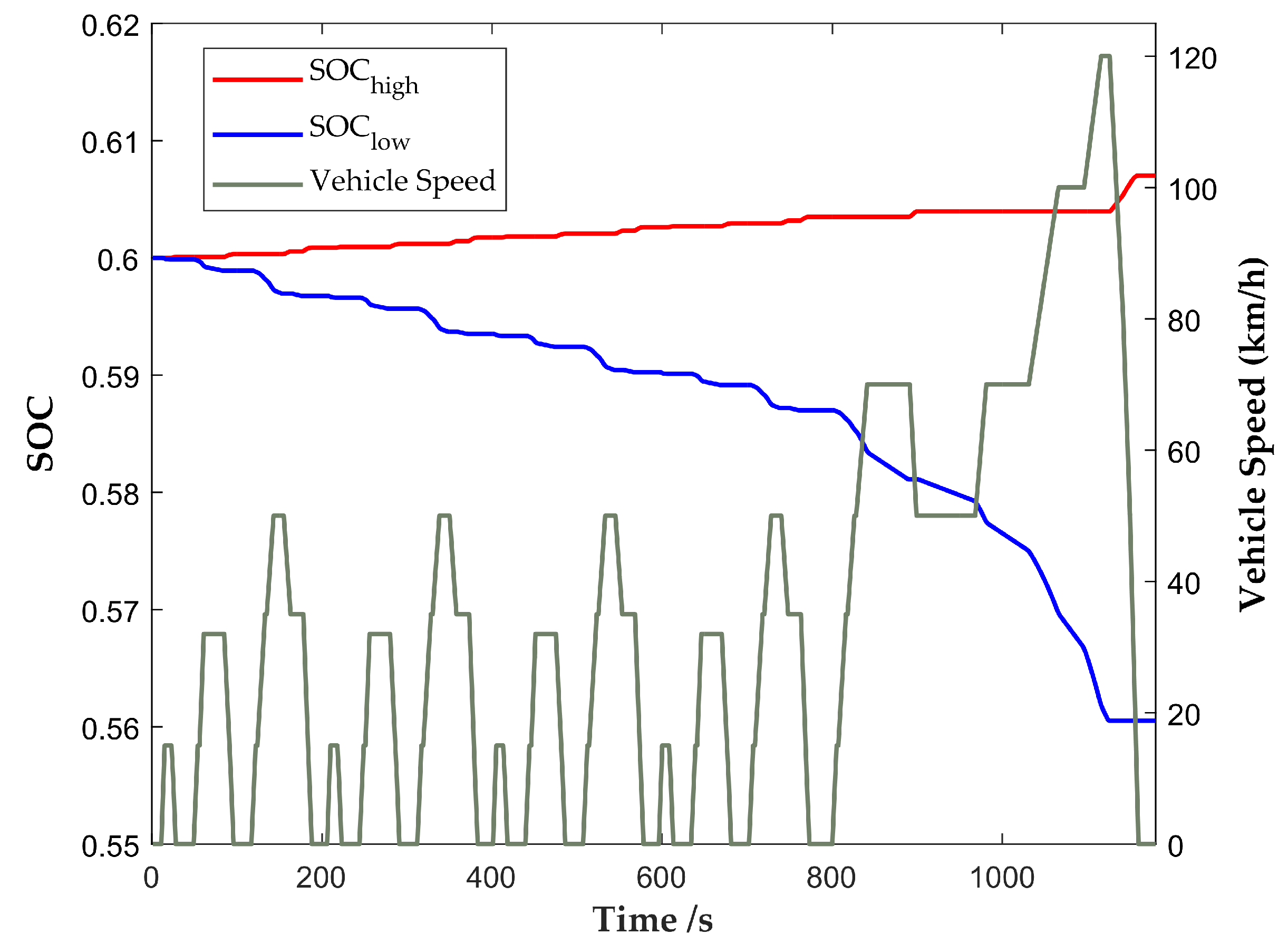
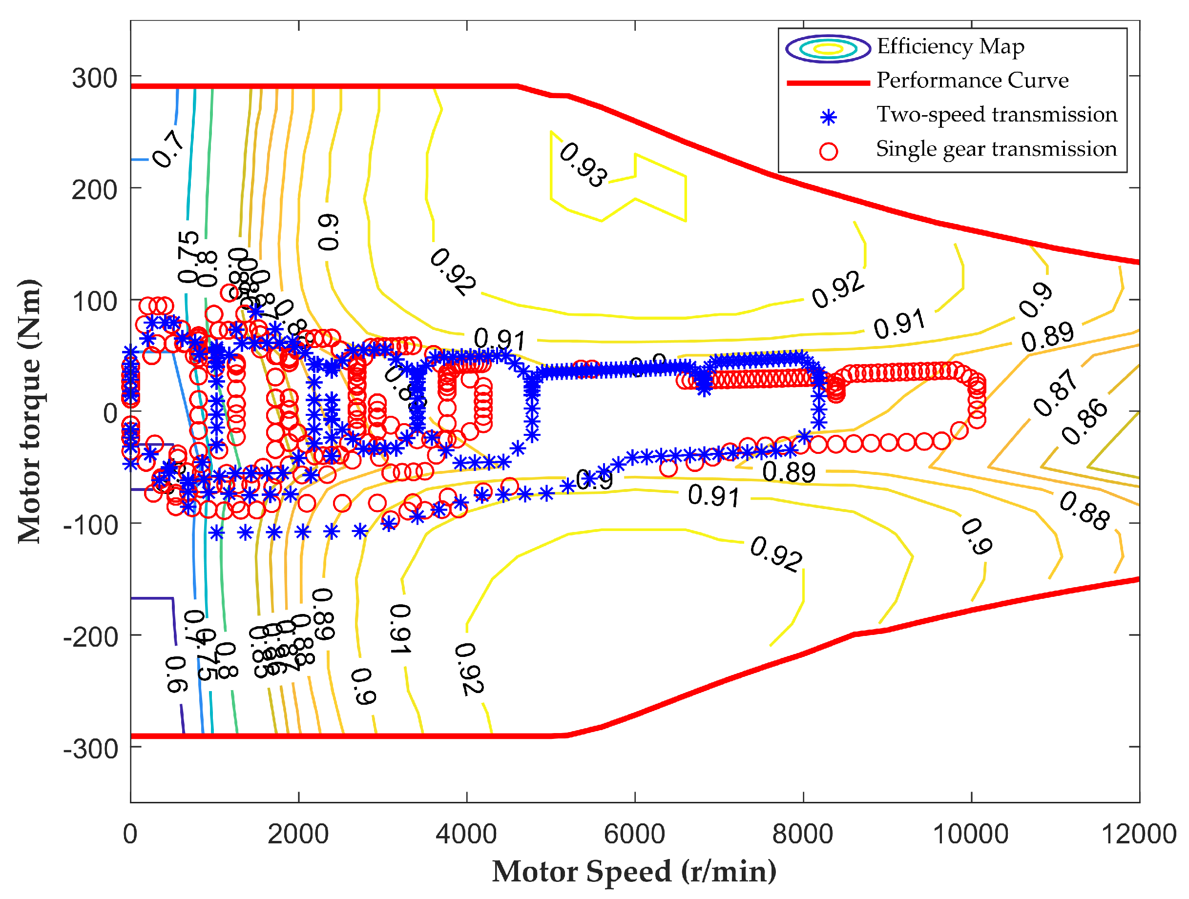
3.2.2. The Electric Energy Consumption

The 100 km electric energy consumption of the EV depends on the specific driving cycle. In order to fully reflect the energy consumption of the electric-drive system, the average of two standard drive cycles, NEDC (New European Drive Cycle) and WLTP (World Light Vehicle Test Procedure), is used as the weighted value of the objective function.
J e l e = S N E D C S N E D C + S W L T P J N E D C * + S W L T P S N E D C + S W L T P J W L T P * ,
where S N E D C and S W L T P is the mileage of NEDC and WLTP respectively, J N E D C * and J W L T P * are the minimum electricity consumption of corresponding drive cycle.
In each iteration process of the optimization process shown in Figure 2, the corresponding gear ratio combination of each individual has been assigned. Thus, given the drive cycle, the 100 km electric energy consumption of the EV is determined by the gear shift sequence. From a control point of view, this is a multistage decision-making process, so DP method can be used to solve this problem [25]. The following is a brief description of the implementation process.
  • The global optimization problem formulation
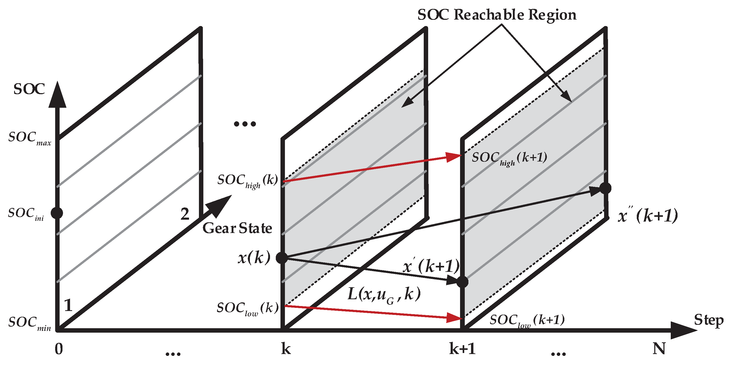
Since the vehicle speed and acceleration are known in the standard drive cycle, the driveline torque and state-of-charge (SOC) of the battery at each time step k can be derived through a backward simulation model. The state-space model of the EV adopting the two-speed transmission can be established in Equation (8).
S O C ( k + 1 ) = S O C ( k ) I ( k ) T s 3600 Q c G ( k + 1 ) = G ( k ) + u G ( k ) ,
where the state variable is x = [ S O C , G ] , G denotes the gear state, T s is the time interval and can be set to 1, Q c is the battery capacity, u G is the only control variable and represents the gearshift command, I is the battery current and can be expressed as follows:
I = V o c V o c 2 4 R i n t P b a t t 2 R i n t
where P b a t t is the battery power related to motor power flow, and V o c and R i n t are open circuit voltage and internal resistance, respectively. The tendency of the battery open circuit voltage with SOC and the battery internal resistance with SOC are shown in Figure 3.
The DP optimization objective is to obtain the minimum electric energy consumption of the whole drive cycle, the cost of applying the control u G ( k ) at time step k can be intuitively defined as
L ( x ( k ) , u G ( k ) , k ) = ψ b a t t ( x ( k ) , u G ( k ) , k ) ,
where ψ b a t t is the electricity consumption during the time interval. In addition, the cost of the frequent shift is considered, thus, Equation (10) is rewritten as
L ( x ( k ) , u G ( k ) , k ) = ψ b a t t ( x ( k ) , u G ( k ) , k ) + w G | u G ( k ) | ,
where w G is the weight coefficient to penalize the frequently gearshift event.
Finally, the objective function can be obtained by integrating the Equation (11) over the entire drive cycle.
J = ϕ ( x ( N ) , N ) + k = 0 N 1 L ( x ( k ) , u G ( k ) , k ) ,
where ϕ ( x ( N ) , N ) is the final cost that is independent of the control variable. In this paper, there is no constraint on the final state, thus, the global optimization problem can be constructed as
min u G J = k = 0 N 1 L ( x ( k ) , u G ( k ) , k ) s . t . S O C m i n S O C ( k ) S O C m a x G ( k ) { 1 , 2 } u G ( k ) { 1 , 0 , 1 } ,
where S O C m a x and S O C m i n are maximum and minimum values of SOC operating range according to the battery management system (BMS).
  • The DP calculation process
    According to Bellman’s optimality principle [25], the global optimization problem can be decomposed into a series of simple minimization problems as follows:
    (a)
    Cost calculation at N 1 step
    J N 1 * x ( N 1 ) = min u G ( N 1 ) { 1 , 0 , 1 } L x ( N 1 ) , u G ( N 1 ) , N 1 .
    (b)
    Intermediate calculation step for k = N 2 to 0
    J k * x ( k ) = min u G ( k ) { 1 , 0 , 1 } L x ( k ) , u G ( k ) , k + J k + 1 * x ( k + 1 ) ,
    where J k + 1 * x ( k + 1 ) represents the minimum objective function from the state variable at the ( k + 1 ) t h step to the state variable at the N t h step. The DP calculation process consists of the backward calculation and forward calculation parts. First, starting from the ( N 1 ) t h step, based on Equations (14) and (15), the minimum objective function for each state variable at the previous step can be derived in an iterative way and the optimal control policy corresponding to this state variable is stored. In the forward calculation process, starting from the initial time and state variable, the optimal control variable at k t h step can be obtained from the optimal control policy stored in the above backward calculation process. Combining Equations (8) and (9), the state variable at the next step on the optimal path can be calculated and the above process is repeated until the final step is reached.
In the optimization procedure shown in Figure 2, the population’s update requires the computation of objective functions for each individual. The DP process needs to be invoked sequentially to calculate the 100 km electric energy consumption, so a fast solution method for DP problem is crucial. If the state variable space is meshed according to S O C m a x and S O C m i n during backward recursion, as the square region of the solid line envelope in Figure 4, some region of the state space cannot be reached during the specific drive cycle, which creates the unnecessary computational burden. In this paper, provided that the initial value of the SOC and drive cycle are known, the reachable region of SOC at any time step k can be calculated in advance, which can help reduce the search scope of the state variable space. The reachable regions of SOC at k t h step and ( k + 1 ) t h step are the gray regions shown in Figure 4.
The SOC range at ( k + 1 ) t h step can be calculated by combining Equations (8) and (9):
S O C h i g h ( k + 1 ) = S O C h i g h ( k ) V o c ( k ) V o c 2 ( k ) 4 R i n t ( k ) P b a t t , m i n ( k ) 7200 R i n t ( k ) Q C S O C l o w ( k + 1 ) = S O C l o w ( k ) V o c ( k ) V o c 2 ( k ) 4 R i n t ( k ) P b a t t , m a x ( k ) 7200 R i n t ( k ) Q C S O C h i g h ( 0 ) = S O C l o w ( 0 ) = S O C i n i ,
where S O C i n i is the initial value of the SOC; S O C h i g h ( k + 1 ) and S O C l o w ( k + 1 ) denote the maximum and minimum value of SOC estimated at ( k + 1 ) t h step, respectively; the open circuit voltage and internal resistance for S O C ( k ) at k step can be obtained from Figure 3; P b a t t , m i n and P b a t t , m a x are the minimum and maximum battery power and can be expressed as follows:
P b a t t , m a x / m i n = P v e h η t o t s g n ( P v e h ) η M s g n ( P v e h ) ,
where P v e h is the vehicle required power based on specific drive cycle, η M is the motor efficiency at k step and varies as a function of motor torque and speed. Since the optimal path has not been obtained at this stage, the gear state at k step is undetermined, thus, the motor torque and speed at k step cannot be derived with the driveline torque and vehicle speed from drive cycle. To simplify the analysis, for the case where P v e h is greater than 0, the value of η M can be replaced by the minimum value from the motor efficiency map; for case where P v e h is smaller than 0, it can be replaced by the maximum value from the motor efficiency map. Figure 5 gives an example of calculating the boundary range of SOC with the initial SOC at 0.6 under NEDC drive cycle.

3.3. Optimization Results and Analysis

The integrated NSGA-II approach described above is used to generate Pareto-optimal solutions for the gear ratio optimization problem. Setting the population size to 100 and the Pareto fraction to 0.3, the Pareto front between the acceleration time from 0 to 100 km/h and the 100 km electricity consumption is shown in Figure 6. From the graph, the 100 km electric energy consumption of the Pareto-optimal solutions have no obvious difference and the range is less than 0.2 kWh/100 km, while the range of the acceleration time corresponding to these solutions is about 1.5 s. Therefore, the point indicated by the pentagram in Figure 6 is chosen as the compromise solution ( [ i 1 , i 2 ] = [ 11.07 , 7.09 ] ) in this paper, where the 100 km electric energy consumption is 12.72 kWh/100 km and the acceleration time is 7.03 s.
In order to reveal the effect of the selected gear ratio combination, Table 3 provides a comparison of the acceleration time and electricity consumption between the two-speed transmission and fixed-ratio transmission. The acceleration time of the EV with two-speed transmission is reduced by 1.15 s compared to the EV with fixed-ratio transmission. In addition, in both the NEDC and WLTP drive cycles, the 100 km electric energy consumption can be reduced by more than 4%.
Take the NEDC drive cycle for example, Figure 7 provides a more intuitive explanation, which shows the motor operating points of the two-speed transmission and the fixed-ratio transmission. As shown in the diagram, the motor operating points of the two-speed transmission are more concentrated in the high-efficiency area, while the motor of the fixed-ratio transmission operates in a larger speed range to meet the vehicle speed requirements of the drive cycle which causes a lower overall efficiency.

4. Gearshift Control Problem

Before designing the gearshift controller, some characteristics of the electric-drive system should be noted: (a) inertia of the motor is much smaller than that of the engine in conventional transmissions; (b) the motor torque is more stable, more responsive, and more precise than the engine torque, which makes accurate speed regulation possible. These facts should be utilized to simplify controller design and facilitate determination of the control scheme.
General requirements for gearshift control of the proposed two-speed transmission are as follows:
  • Duration of the whole process can be easily manipulated.
  • Jerks on both the input and output shaft are small enough so as to protect the motor shaft and ensure riding comfort.
  • Friction work of the two brakes are small enough so as to protect the two components.
  • Output torque of the transmission can be arbitrarily shaped (within the capability and constraint of components) during the shifting process so as to ensure drivability on some high-performance models.
The shifting process of 1–2 upshift is considered in this paper and the clutch-to-clutch shifting process can be divided into two phases: the torque phase (to execute the clutch’s torque transfer) and the inertia phase (to execute the clutch speed synchronizing).

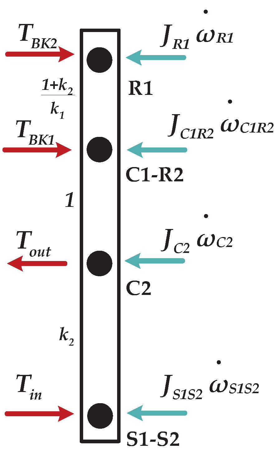
4.1. Mathematical Model of the Electrified Power-Train

The dynamics of the power train can be modeled via the Lever-analogy method [22]. The Level diagram of the two-speed transmission is shown in Figure 8.
T B K 1 + T B K 2 + T i n T o u t J R 1 ω ˙ R 1 J C 1 R 2 ω ˙ C 1 R 2 J C 2 ω ˙ C 2 J S 1 S 2 ω ˙ S 1 S 2 = 0 ( 1 + k 2 ) ( T B K 2 J R 1 ω ˙ R 1 ) + k 1 ( T o u t + J C 2 ω ˙ C 2 ) + ( k 1 + k 2 ) ( J S 1 S 2 ω ˙ S 1 S 2 T i n ) = 0 k 1 ω R 1 + ω S 1 S 2 ( 1 + k 1 ) ω C 1 R 2 = 0 k 2 ω C 1 R 2 + ω S 1 S 2 ( 1 + k 2 ) ω C 2 = 0 ,
where T x ( x = B K 1 , B K 2 , i n , o u t ) denote the transmitted torque of the two brakes and the input and output torque, respectively; ω ˙ x ( x = R 1 , C 1 R 2 , C 2 , S 1 S 2 ) present the respective angular acceleration; J x ( x = R 1 , C 1 R 2 , C 2 , S 1 S 2 ) refer to the inertia of the components of the planetary gear sets and J S 1 S 2 is the lumped inertia on the input shaft which include those of the motor itself and the first and second sun gears; and J C 2 is the lumped inertia on the output shaft including those of the carriers, the vehicle body, and the wheels.
To facilitate controller design and analysis, the dynamic model is further simplified by ignoring the inertias that do not connect directly with the input and output shaft:
J S 1 S 2 ω ˙ S 1 S 2 = T i n 1 k 2 T B K 1 1 + k 1 + k 2 k 1 k 2 T B K 2
J C 2 ω ˙ C 2 = T o u t + 1 + k 2 k 2 T B K 1 + 1 + k 1 + k 2 + k 1 k 2 k 1 k 2 T B K 2 .

4.2. Torque Phase Control

In the torque phase, the load on the motor shaft should be gradually transferred from the off-going brake to the oncoming one.
Requirements for torque phase control are as follows:
  • The off-going brake should be kept engaged during the whole process and no slip occurs.
  • The load and the pressure on the off-going brake should be reduced to zero at the same time.
Under the first gear, BK1 is locked, which results in
ω ˙ S 1 S 2 = ( 1 + k 2 ) ω ˙ C 2 ,
where ω ˙ C 2 can be expressed with T o u t , T B K 2 , and T i n by solving Equations (19)–(21):
ω ˙ C 2 = 1 ( 1 + k 2 ) 2 J S 1 S 2 + J C 2 ( 1 + k 2 ) T i n T o u t 1 + k 2 k 1 T B K 2 .
The inertia of the motor is rather small compared to that of the engine, and therefore J S 1 S 2 can be neglected. Based on this assumption, Equation (22) is simplified as
J C 2 ω ˙ C 2 = ( 1 + k 2 ) T i n 1 + k 2 k 1 T B K 2 T o u t .
Thus, the driving torque on the output shaft is
T d r i v = ( 1 + k 2 ) T i n 1 + k 2 k 1 T B K 2 .
Note that T d r i v consists of two terms regarding T i n and T B K 2 . The former is the motor torque; and the latter is determined by the pressure on BK2 (since it is slipping during the torque phase). Thus, T d r i v can be manipulated either through controlling the motor or BK2. As an internal torque, T B K 1 is determined by T i n and T B K 2 as well:
T B K 1 = k 2 T i n 1 + k 1 + k 2 k 1 T B K 2 .
During the torque phase, there are totally three components to be controlled, namely, the motor and two brakes. However, according to Equations (24) and (25), only one variable can be freely determined.
Recalling the requirement on controllability of the shift time, T B K 1 (transmitted torque of the off-going brake) should better be selected as the one being manipulated. For example, as the simplest case, T B K 1 can be commanded to decrease to zero linearly within a specified duration. Since BK1 is required to be kept engaged along the whole torque phase, its transmitted torque should be no larger than the torque capacity T c a p , B K 1 .
T B K 1 T c a p , B K 1 .
Additionally, recall the second requirement that T B K 1 and T c a p , B K 1 be reduced to zero at the same time, which suggests the following control law for T B K 1 :
T B K 1 = λ T c a p , B K 1 ,
where λ is a coefficient that satisfies λ 1 . For practical use, λ is advised to fall between 0.90 and 0.99. As has been discussed before, the trajectory of T c a p , B K 1 in torque phase can be designed as a linear curve:
T c a p , B K 1 = T c a p , B K 1 ( t 0 ) T c a p , B K 1 ( t 0 ) t 1 t 0 ( t t 0 ) , t 0 t t 1 ,
where t 0 and t 1 are the start and end point of the torque phase, respectively. Duration of the torque phase can thus be arbitrarily manipulated (within the capacity and constraint of components) through the parameter t 1 . T d r i v in Equation (24) is specified by the vehicle controller unit (VCU) and related to position of the accelerator pedal. Therefore, it can be treated as known. T i n and T B 2 can be derived by solving Equations (24) and (25):
T B K 2 = k 1 k 2 1 + k 1 + k 2 + k 1 k 2 T d r i v k 1 1 + k 1 T B K 1
T i n = 1 + k 1 + k 2 1 + k 1 + k 2 + k 1 k 2 T d r i v 1 1 + k 1 T B K 1 .
Equations (27)–(30) are control laws for the torque phase. It should be noted that the T c a p , B K 1 ( t 0 ) in Equation (28) should be determined carefully, so as not to cause sudden change of T i n and T B K 2 . Combining Equations (25) and (27), the transmitted torque capacity of BK1 at the beginning of the torque phase is
T c a p , B K 1 ( t 0 ) = k 2 λ T i n ( t 0 ) .
This is the exact level that the pressure of BK1 should be reduced to during the filling phase which precedes the torque phase.

4.3. Inertia Phase Control

At the end of the torque phase, BK2 is still slipping and speeds of its two sides need to be synchronized. Note that in the inertia phase, BK1 is fully disengaged, and therefore the driving torque on the output shaft is solely determined by the pressure on BK2. Recalling the constant-output-torque requirement, BK2 should remain constant along the whole inertia phase (assuming that T d r i v is constant):
T B K 2 ( t ) = k 1 k 2 1 + k 1 + k 2 + k 1 k 2 T d r i v ( t ) , t 1 t t f ,
where t f denotes the end of inertia phase. Since BK1 is totally disengaged in this phase, the motor is the sole component to be controlled for speed synchronization. This approach is reasonable in that it fully exploits advantages from the precise output torque as well as fast response of the motor.
The key of inertia phase control is to realize a fast (in terms of the duration) and comfortable (in terms of longitudinal jerk felt by the passengers) speed ratio change. Common practice is to make the slip speed of the oncoming brake follow a polynomial curve. According to the GV no-lurch condition [26], the derivative of the slip speed at the synchronization point should be zero so as to avoid sudden change of T B K 2 ; it can be expressed as
Δ ω ˙ R 1 ( t f ) = 0 .
To accomplish this, a fifth-degree polynomial is selected as the slip speed reference and can be expressed as follows:
ω R 1 ( t ) = ω R 1 ( t 1 ) 1 s ( t ) s ( t ) = a 5 t t 1 t f t 1 5 a 4 t t 1 t f t 1 4 + a 3 t t 1 t f t 1 3 ,
where a i ( i = 5 , 4 , 3 ) denote the polynomial coefficients, ω R 1 ( t 1 ) can be expressed as
ω R 1 ( t 1 ) = 1 + k 1 + k 2 + k 1 k 2 k 1 k 2 ω C 2 ( t 1 ) 1 + k 1 + k 2 k 1 k 2 ω S 1 S 2 ( t 1 ) ,
where ω C 2 ( t 1 ) and ω S 1 S 2 ( t 1 ) can be obtained from the speed sensors in the input and output shaft of the transmission.

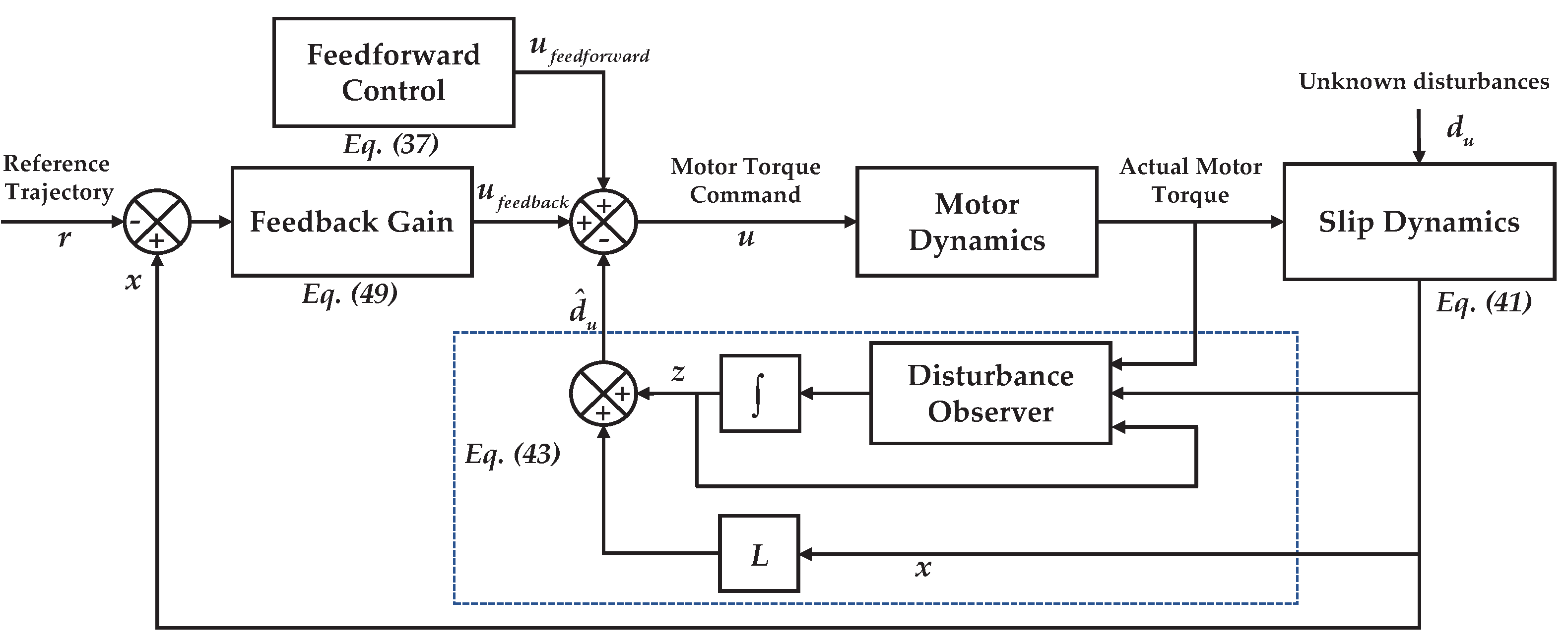
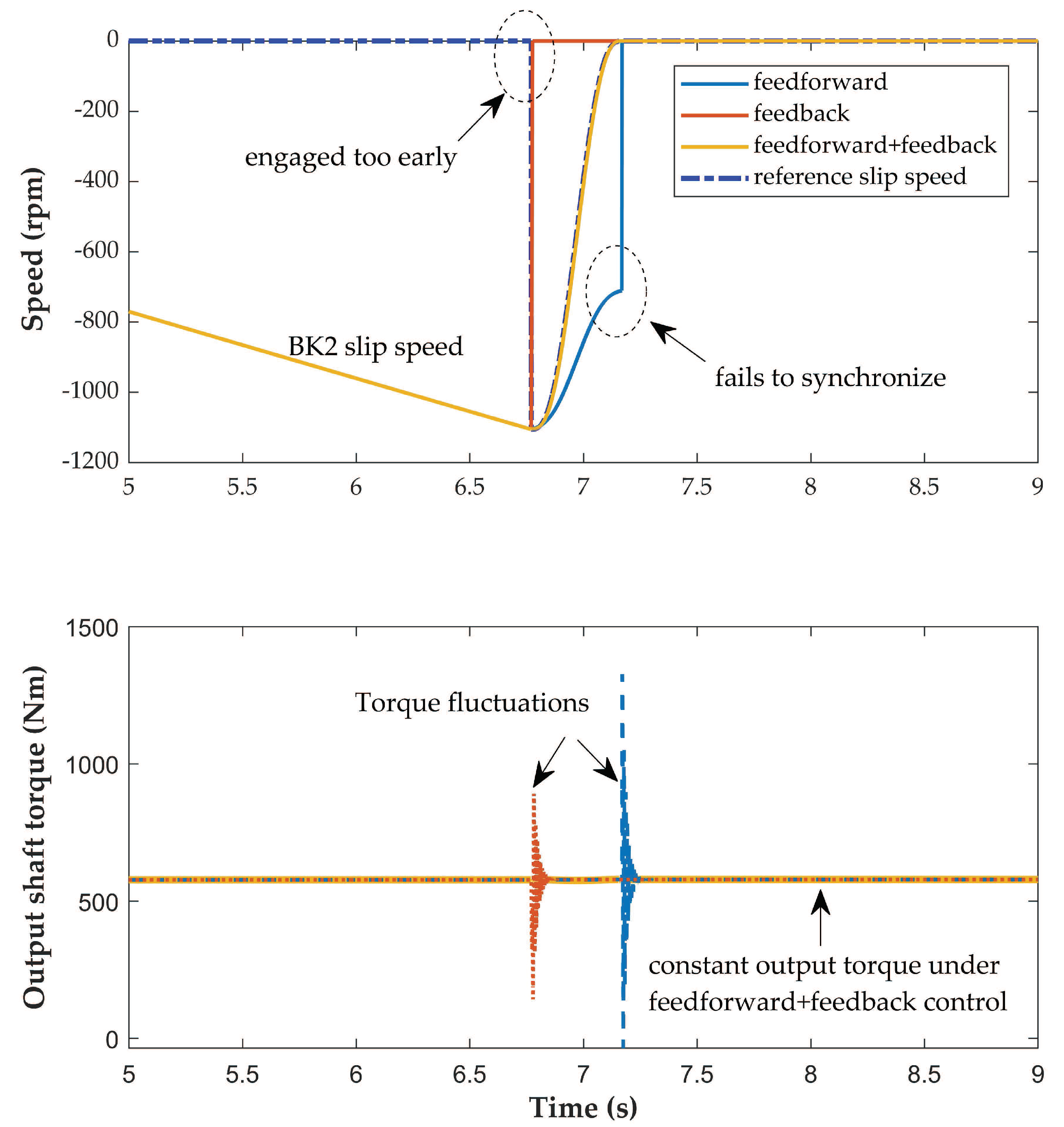
4.3.1. Feedforward Control

The feedforward–feedback control scheme is adopted to solve the tracking problem of the slip speed. Firstly, the inverse kinetic model of the two-speed transmission should be derived. ”Inverse“ means that the rotational acceleration of the input shaft ω ˙ S 1 S 2 is taken as known while the input torque T i n is taken as unknown. In the inertia phase, the two-speed transmission is in the neutral gear state, and the forward kinetic model requires typically four quantities known for solution, namely, T i n , T B K 1 , T B K 2 , and T o u t . In the inverse model, T i n and T o u t are substituted by ω ˙ S 1 S 2 and ω ˙ R 1 , respectively. T B K 1 equals to zero along the whole inertia phase as a result of total disengagement of BK1. The aim now is to answer the question ”given ω ˙ S 1 S 2 , ω ˙ R 1 , and T B K 2 , how do we determine T i n ?“. Among them, ω ˙ S 1 S 2 can be attained through an acceleration estimator over the motor speed, which is reported by the motor controller unit (MCU). ω ˙ R 1 is from the designed trajectory in Equation (34) and should be apparently known. As has been discussed before, during the inertia phase, T d r i v is determined by T B K 2 only, and therefore T B K 2 can be calculated from Equation (32). Thus, T i n is determined as follows:
T i n = 1 + k 1 + k 2 1 + k 1 + k 2 + k 1 k 2 T d r i v + J S 1 S 2 1 k 2 + k 1 k 2 J C 1 R 2 ω ˙ S 1 S 2 1 + k 1 + k 2 k 1 k 2 J R 1 + k 1 k 2 + k 1 k 2 J C 1 R 2 ω ˙ R 1 .
Equation (36) is the feedforward control law for T i n . Note that according to Equation (34), ω ˙ R 1 ( t 1 ) = 0 . As a result, T i n ( t 1 ) = 1 + k 1 + k 2 1 + k 1 + k 2 + k 1 k 2 T d r i v ( t 1 ) , which is exactly the same as Equation (30). This implies that value of T i n at the end of the torque phase and at the beginning of the inertia phase are the same. Thus, continuity of the motor torque is ensured.
Considering that inertias J S 1 S 2 and J C 1 R 2 are small and negligible, the second term regarding ω ˙ S 1 S 2 in Equation (36) can be omitted. This also cancels the acceleration observer and simplifies the controller. The final feedforward control law is
T i n = 1 + k 1 + k 2 1 + k 1 + k 2 + k 1 k 2 T d r i v 1 + k 1 + k 2 k 1 k 2 J R 1 + k 1 k 2 + k 1 k 2 J C 1 R 2 ω ˙ R 1 .

4.3.2. Feedback Control

To derive the feedback control law, the forward kinetic model should be used. However, as has been discussed before, T o u t is the load on the wheel and is hard to measure. It should be substituted by ω ˙ S 1 S 2 , which can be attained indirectly. As before, substituting T B K 2 with T d r i v , ω ˙ R 1 can be expressed as Equation (38).
ω ˙ R 1 = 1 ρ { ( 1 + k 1 + k 2 ) k 1 k 2 T d r i v ( 1 + k 1 ) ( 1 + k 2 ) k 1 k 2 T i n + ( 1 + k 1 + k 2 ) k 1 k 2 J S 1 S 2 ( 1 + k 2 ) k 1 J C 1 R 2 ω ˙ S 1 S 2 } ,
where
ρ = ( 1 + k 1 + k 2 ) ( 1 + k 1 ) ( 1 + k 2 ) J R 1 + ( 1 + k 2 ) k 1 2 J C 1 R 2 .
From Equation (38), it is obvious that ω ˙ R 1 is related to three quantities, namely, T d r i v , T i n , and ω ˙ S 1 S 2 . If the term regarding ω ˙ S 1 S 2 is omitted, Equation (38) turns into
ω ˙ R 1 = 1 ρ ( 1 + k 1 + k 2 ) k 1 k 2 T d r i v ( 1 + k 1 ) ( 1 + k 2 ) k 1 k 2 T i n .
The term regarding T d r i v can be treated as known disturbances and compensated in a feedforward way. To make it clear, rewrite Equation (38) in the state-space form:
x ˙ = a x + b u + b k d k + b u d u
with
x = ω R 1 a = 0 u = T i n b = ( 1 + k 1 ) ( 1 + k 2 ) k 1 k 2 ρ b k d k = ( 1 + k 1 + k 2 ) k 1 k 2 ρ T d r i v ,
where d k and d u denote known and unknown disturbances, respectively. With b u = b , a time-domain disturbance observer (DO) can be used to estimate d u :
z ˙ = L b ( z + L x ) L ( a x + b u + b k d k ) d ^ u = z + L x .
Note that L should satisfy L b < 0 . The component for disturbance compensation in u is as follows:
u d u = d ^ u .
Note that u f e e d f o r w a r d in Equation (37) can be written as follows:
u f e e d f o r w a r d = u d u + u i n v ,
where
u d k = b k d k b = 1 + k 1 + k 2 1 + k 1 + k 2 + k 1 k 2 T d r i v
u i n v = 1 + k 1 + k 2 k 1 k 2 J R 1 + k 1 k 2 + k 1 k 2 J C 1 R 2 ω ˙ R 1 ,
where u d k is used to compensate the known disturbances b k d k , while u i n v is derived from the nominal model. Assuming that both b k d k and b u d u are completely compensated, the state-space model in Equation (41) turns into the nominal one and can be expressed as follows:
x ˙ n = a x n + b u n .
The feedback control law for the nominal model is
u f e e d b a c k = F ( x r ) ,
where F is the feedback gain and can be roughly determined as
F = ln | ω R 1 ( t 1 ) | ln E b ( t f t 1 ) ,
where E is the level of residual tracking error when t f is reached. Note that the sign of F should be determined in accordance with a and b to ensure convergence. This is obvious by substituting Equation (49) into (48), whose solution is
x n ( t ) = x n ( t 1 ) + b F a b F e ( a b F ) t b F a b F r ,
where the reference signal r is from the fifth-degree polynomial expressed by Equation (34).
For the exponential convergence of x n ( t ) to x n ( ) = b F a b F r , F should satisfy that
a b F < 0 .
Finally, the control law for T i n in the inertia phase can be summarized as
u = u d k + u i n v + u d u + u f e e d b a c k .
Block diagram of the slip speed controller is shown in Figure 9.

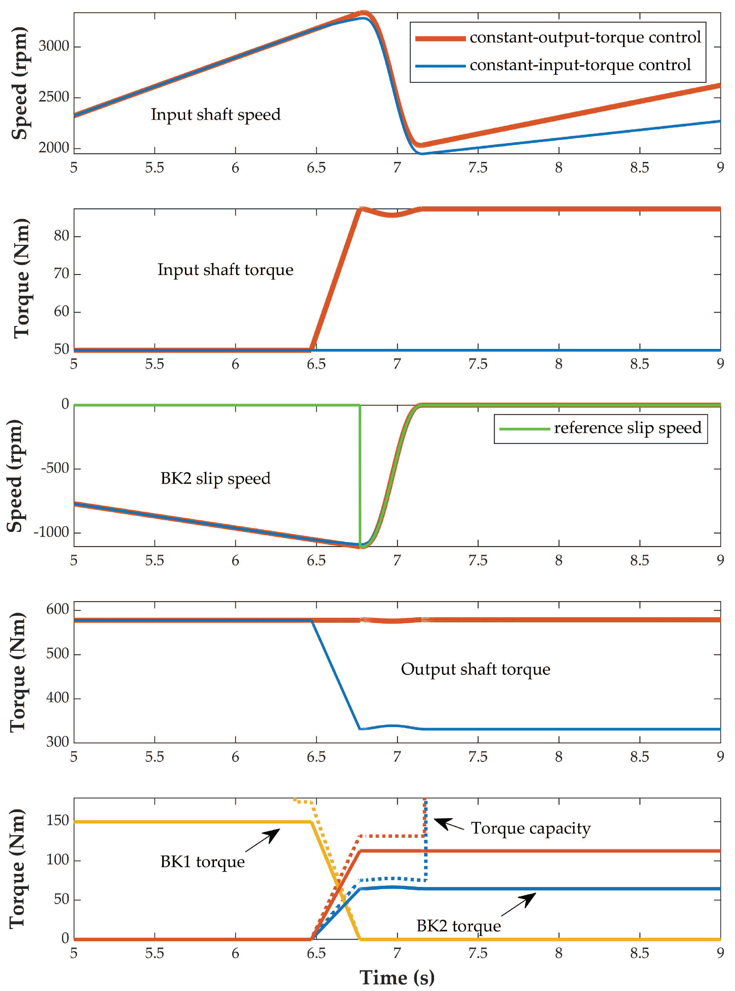
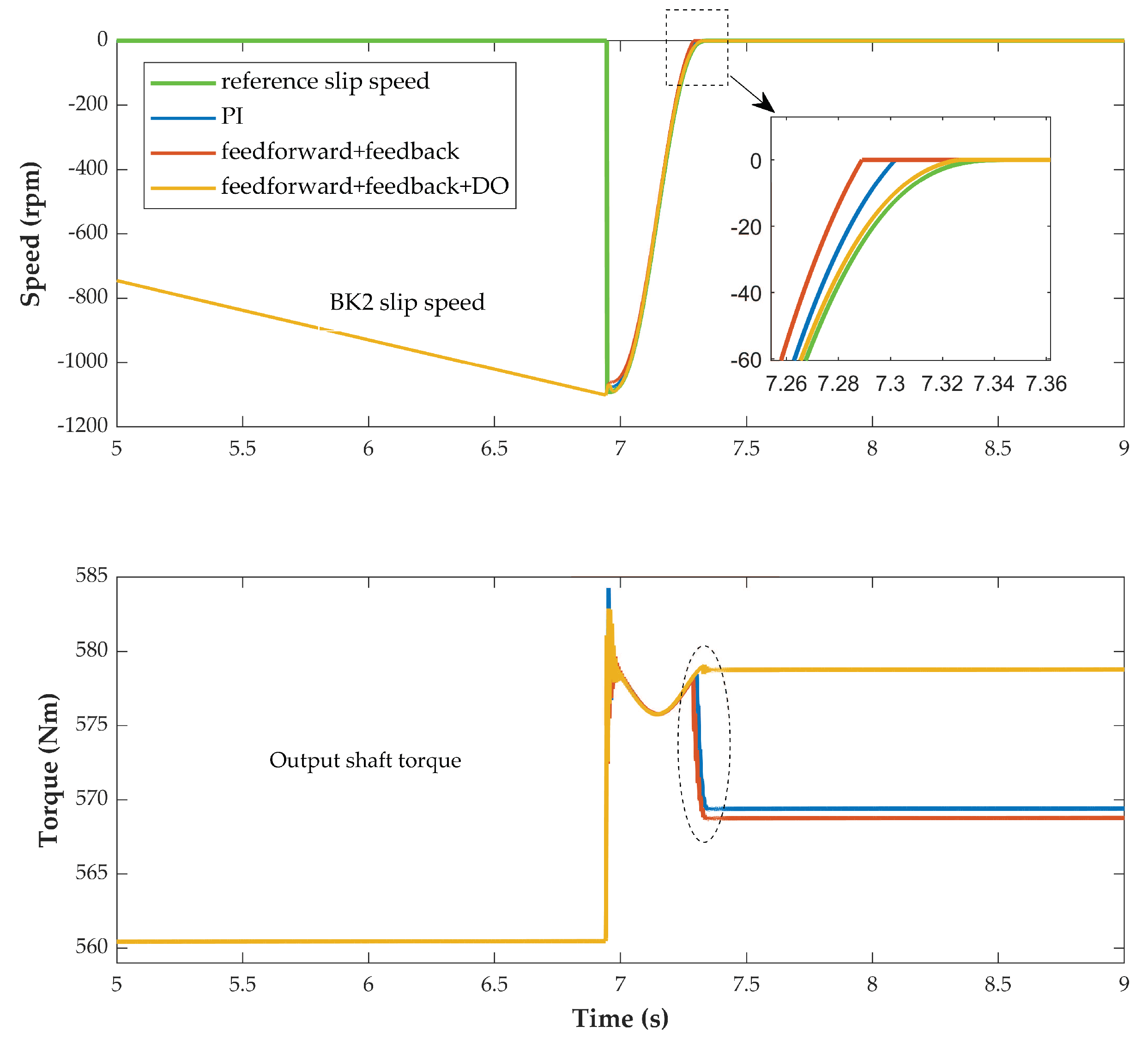
4.4. Simulation Results

A model is developed in MATLAB/SIMULINK (version R2018a) to validate the proposed feedforward–feedback shift controller with disturbance compensation. It mainly consists of four parts: submodels for the motor, the transmission, the vehicle body, and the shift controller. Stiffness and damping on the output shafts are taken into consideration. Firstly, the constant-output-torque control (COTC) is compared to the conventional constant-input-torque control (CITC), which keeps the input shaft torque constant along the whole shifting process. Simulation results are shown in Figure 10. In COTC, during the torque phase, the motor torque is increased to compensate the reduction of output torque due to the change of gear ratio. In contrast, CITC simply maintains the motor torque. As a result, the output shaft torque decreases during the upshift. The pressure level of the oncoming brake in COTC is higher than that of CITC to keep the output torque constant. In the inertia phase, COTC relies on the motor torque for slip speed regulation, whereas CITC changes the pressure of the oncoming brake to accomplish this.
Advantages of the feedforward–feedback scheme are validated through comparison with pure feedforward and feedback ones, as are shown in Figure 11. Both pure feedback and feedforward control fail to follow the slip speed reference. Under the pure feedback one, the slip speed falls to zero quickly and its derivative fails to meet the GV no-lurch condition at the synchronization point. As a result, significant torque fluctuations are observed on the output shaft. For the pure feedforward control, since model simplification is applied in derivation of the control law, the tracking error is quite large at the end of the interval, and there are also output torque fluctuations. On the other hand, if the feedforward and the feedback control are combined, the slip speed reference is then well followed and the output torque is successfully kept constant and smooth.
Simulations above are based on the nominal model, i.e., there are no disturbances. Necessity of the disturbance observer is evaluated by adding a friction torque (1.5 Nm) on the input shaft. Performances of the three controllers are compared, namely, the conventional proportional–integral control (PI), the feedforward–feedback control, and the feedforward–feedback control with disturbance compensation. Tuning of the PI controller is a time-consuming process, and in this paper, we set the proportional gain to be consistent with the feedback control. We perform simulations multiple times with different integrating gains and take the parameter values corresponding to the best results. The proportional and integrating gains are set to be 0.5 and 1, respectively, in this test scenario. Results are shown in Figure 12. As can be seen, all the three controllers follow the slip speed reference generally well. However, at the synchronization point (when the rotational speed of the oncoming brake decreases to zero), slip speed from the feedforward–feedback controller with DO comes with a more ”gentle landing“ (derivative of the slip speed has a smaller magnitude) than those of the other two. Consequently, the driving torque on the output shaft is smoother and without a sudden change (though it is small for PI and feedforward–feedback without DO). Therefore, for practical engineering use where there is bound to be unknown disturbances and uncertainties, DO should always be integrated in the controller.

5. Summary and Conclusions

This paper proposes a two-speed transmission based on dual planetary gear sets for EVs, and the gear ratio optimization and gearshift control problems of the two-speed transmission are studied. The main results can be summarized as follows:
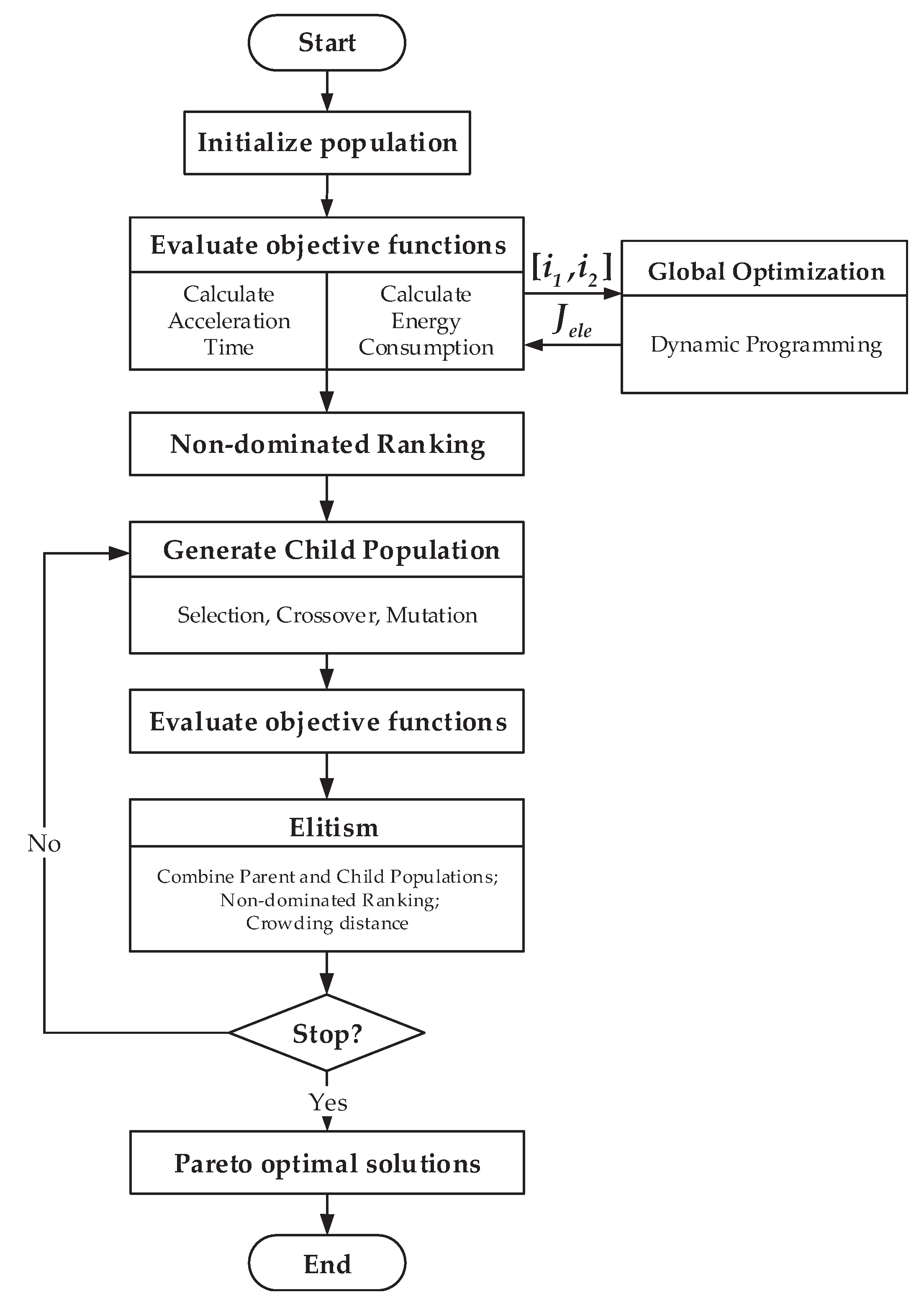
  • From the Pareto front graph obtained using the NSGA-II approach, the dynamic and economic performance of the two-speed transmission is conflicted with the other. Thus, a compromise solution is chosen as the final gear ratio combination.
  • Simulation results demonstrate that the two-speed transmission has much better performance in terms of acceleration time and electric energy consumption compared with the fixed-ratio transmission.
  • Compared with the conventional constant-input-torque control (CITC), the proposed constant-output-torque control (COTC) comes with advantages of keeping the driving torque on the output shaft constant during the whole gearshift process.
  • The disturbance observer is integrated to the feedforward–feedback slip speed controller to enhance the robustness, and the effectiveness is validated through comparison with the non-disturbance-compensation method. Thus, the controller is suitable for practical engineering use.
The proposed control scheme is also applicable to other clutch-to-clutch shift-based transmissions. Our future work directions include the mechanical structure development of this transmission and the validation of the proposed gearshift method through bench and real vehicle tests.

Author Contributions

Conceptualization, W.H. and J.H.; data curation, W.H.; funding acquisition, C.Y.; methodology, W.H. and J.H.; project administration, C.Y.; validation, W.H. and J.H.; writing—original draft, W.H. and J.H.; writing—review & editing, C.Y. All authors have read and agreed to the published version of the manuscript.

Funding

This research was funded by the National Key Technology R & D Program of China, grant number 2015BAG04B01.

Conflicts of Interest

The authors declare no conflict of interest.

Abbreviations

The following abbreviations are used in this manuscript:
EVElectric vehicle
NSGA-IINondominated sorting genetic algorithm-II
DPDynamic programming
COTCConstant-output-torque control
DCTEquivalent inertia of the transmission output shaft
CVTContinuous variable transmission
ATAutomatic transmission
AMTAutomatic manual transmission
HMPHybrid minimum principle
PGTsPlanetary-gear-based transmissions
DOFDegree of freedom
NEDCNew European Drive Cycle
WLTPWorld Light Vehicle Test Procedure
SOCState-of-charge
BMSBattery management system
VCUVehicle controller unit
MCUMotor controller unit
DODisturbance observer
CITCConstant-input-torque control
PIDProportional-integral-derivative
PIProportional–integral

References

  1. Wang, N.; Tang, L.; Pan, H. A global comparison and assessment of incentive policy on electric vehicle promotion. Sustain. Cities Soc. 2019, 44, 597–603. [Google Scholar] [CrossRef]
  2. Ruan, J.; Walker, P.D.; Zhang, N. A comparative study energy consumption and costs of battery electric vehicle transmissions. Appl. Energy 2016, 165, 119–134. [Google Scholar] [CrossRef] [Green Version]
  3. Roberts, S. Multispeed transmission for electric vehicles. ATZ Worldw. 2012, 114, 8–11. [Google Scholar] [CrossRef]
  4. Nicola, F.D.; Sorniotti, A.; Holdstock, T.; Viotto, F.; Bertolotto, S. Optimization of a multiple-speed transmission for downsizing the motor of a fully electric vehicle. SAE Int. J. Altern. Powertrains 2012, 1, 134–143. [Google Scholar] [CrossRef]
  5. Bottiglione, F.; De Pinto, S.; Mantriota, G.; Mantriota, A. Energy Consumption of a Battery Electric Vehicle with Infinitely Variable Transmission. Energies 2014, 7, 8317–8337. [Google Scholar] [CrossRef] [Green Version]
  6. Gao, B.; Liang, Q.; Xiang, Y.; Guo, L.; Chen, H. Gear ratio optimization and shift control of 2-speed I-AMT in electric vehicle. Mech. Syst. Signal Proc. 2015, 50, 615–631. [Google Scholar] [CrossRef]
  7. Ahssan, R.; Ektesabi, M.; Gorji, S.A. Electric Vehicle with Multi-Speed Transmission: A Review on Performances and Complexities. SAE Int. J. Altern. Powertrains 2018, 7, 169–181. [Google Scholar] [CrossRef]
  8. Walker, P.D.; Zhu, B.; Zhang, N. Powertrain dynamics and control of a two speed dual clutch transmission for electric vehicles. Mech. Syst. Signal Proc. 2017, 85, 1–15. [Google Scholar] [CrossRef] [Green Version]
  9. Hong, S.; Son, H.; Lee, S.; Park, J.; Kim, K.; Kim, H. Shift control of a dry-type two-speed dual-clutch transmission for an electric vehicle. Proc. Inst. Mech. Eng. Part D J. Automob. Eng. 2016, 230, 308–321. [Google Scholar] [CrossRef]
  10. Pakniyat, A.; Caines, P.E. Hybrid optimal control of an electric vehicle with a dual-planetary transmission. Nonlinear Anal. Hybrid Syst. 2017, 25, 263–282. [Google Scholar] [CrossRef]
  11. Mo, W.; Walker, P.D.; Fang, Y.; Wu, J.; Ruan, J.; Zhang, N. A novel shift control concept for multi-speed electric vehicles. Mech. Syst. Signal Proc. 2018, 112, 171–193. [Google Scholar] [CrossRef]
  12. Zhu, X.; Zhang, H.; Xi, J.; Wang, J.; Fang, Z. Robust speed synchronization control for clutchless automated manual transmission systems in electric vehicles. Proc. Inst. Mech. Eng. Part D J. Automob. Eng. 2014, 229, 424–436. [Google Scholar] [CrossRef]
  13. Walker, P.D.; Fang, Y.; Zhang, N. Dynamics and Control of Clutchless Automated Manual Transmissions for Electric Vehicles. J. Vib. Acoust. 2017, 139, 61005–61017. [Google Scholar] [CrossRef]
  14. Sorniotti, A.; Subramanyan, S.; Turner, A.; Cavallino, C.; Viotto, F.; Bertolotto, S. Selection of the Optimal Gearbox Layout for an Electric Vehicle. SAE Int. J. Engines 2011, 4, 1267–1280. [Google Scholar] [CrossRef]
  15. Schwarzer, V.; Ghorbani, R. Drive Cycle Generation for Design Optimization of Electric Vehicles. IEEE Trans. Veh. Technol. 2013, 62, 89–97. [Google Scholar] [CrossRef]
  16. Mousavi, M.S.R.; Pakniyat, A.; Boulet, B. Dynamic modeling and controller design for a seamless two-speed transmission for electric vehicles. In Proceedings of the IEEE International Conference on Control Applications (CCA), Antibes, France, 8–10 October 2014; pp. 635–640. [Google Scholar]
  17. Mousavi, M.S.R.; Pakniyat, A.; Wang, T.; Boulet, B. Seamless dual brake transmission for electric vehicles: Design, control and experiment. Mech. Mach. Theory 2015, 94, 96–118. [Google Scholar] [CrossRef]
  18. Roozegar, M.; Angeles, J. A two-phase control algorithm for gear-shifting in a novel multi-speed transmission for electric vehicles. Mech. Syst. Signal Proc. 2018, 104, 145–154. [Google Scholar] [CrossRef]
  19. Gao, B.; Xiang, Y.; Chen, H.; Liang, Q.; Guo, L. Optimal Trajectory Planning of Motor Torque and Clutch Slip Speed for Gear Shift of a Two-Speed Electric Vehicle. J. Dyn. Syst. Meas. Control 2015, 137, 61016–61024. [Google Scholar] [CrossRef] [Green Version]
  20. Roozegar, M.; Angeles, J. The optimal gear-shifting for a multi-speed transmission system for electric vehicles. Mech. Mach. Theory 2017, 116, 1–13. [Google Scholar] [CrossRef]
  21. Mousavi, M.S.R.; Pakniyat, A.; Helwa, M.K.; Boulet, B. Observer-Based Backstepping Controller Design for Gear Shift Control of a Seamless Clutchless Two-Speed Transmission for Electric Vehicles. In Proceedings of the IEEE Vehicle Power and Propulsion Conference (VPPC), Montreal, QC, Canada, 19–22 October 2015; pp. 1–6. [Google Scholar]
  22. Kahraman, A.; Ligata, H.; Kienzle, K.; Zini, D.M. A Kinematics and Power Flow Analysis Methodology for Automatic Transmission Planetary Gear Trains. J. Mech. Des. 2004, 126, 1071–1081. [Google Scholar] [CrossRef]
  23. Deb, K.; Agrawal, S.; Pratap, A.; Meyarivan, T. A fast and elitist multiobjective genetic algorithm: NSGA-II. IEEE Trans. Evol. Comput. 2002, 6, 182–197. [Google Scholar] [CrossRef] [Green Version]
  24. Naunheimer, H.; Fietkau, P. Automotive Transmissions. Fundamentals, Selection, Design and Application; Springer: Heidelberg, Germany, 2011. [Google Scholar]
  25. Bertsekas, D.P. Dynamic Programming and Optimal Control: Volumes I and II; Athena Scientific: Belmont, MA, USA, 2005. [Google Scholar]
  26. Garofalo, F.; Glielmo, L.; Iannelli, L.; Vasca, F. Smooth engagement for automotive dry clutch. In Proceedings of the IEEE Conference on Decision & Control (CDC), Orlando, FL, USA, 4–7 December 2001; pp. 529–534. [Google Scholar]
Figure 1. Layout of the two-speed transmission drivetrain: (a) Diagram of the electric power-train; (b) Cross-sectional view of the virtual prototype of the electric power-train (EM—Electric motor; BK1—First gear brake assembly; R1—First ring gear; C1—First carrier; S1—First sun gear; P1—First planet gears; BK2—Second gear brake assembly; R2—Second ring gear; C2—Second carrier; S2—Second sun gears; P2—Second planet gears).
Applsci 10 06612 g001
Figure 2. Flowchart of the gear ratio optimization procedure with the Nondominated sorting genetic algorithm-II (NSGA-II) approach.
Applsci 10 06612 g002
Figure 3. Battery parameters: (a) The relationship between V o c and state-of-charge (SOC) under charging or discharging status. (b) The relationship between R i n t and SOC under charging or discharging status.
Applsci 10 06612 g003
Figure 4. Determine the SOC reachable region during the Dynamic Programming (DP) calculation process.
Applsci 10 06612 g004
Figure 5. The boundary range of SOC with the initial SOC at 0.6 for New European Drive Cycle (NEDC) drive cycle.
Applsci 10 06612 g005
Figure 6. The Pareto front graph between the acceleration time and electricity consumption.
Applsci 10 06612 g006
Figure 7. The motor operating points in NEDC drive cycle.
Applsci 10 06612 g007
Figure 8. Lever diagram of the two-speed transmission.
Applsci 10 06612 g008
Figure 9. Schematic diagram of the feedforward–feedback slip speed controller.
Applsci 10 06612 g009
Figure 10. Comparison with constant-input-shaft torque control.
Applsci 10 06612 g010
Figure 11. Comparison with pure feedforward and feedback controller.
Applsci 10 06612 g011
Figure 12. Comparison with non-disturbance-observer (DO)-based controllers.
Applsci 10 06612 g012
Table 1. Gear states for the two-speed transmission.
Gear StateBrake StatusLevel AnalogyGear Ratio
1st GearBK1:engaged
BK2:disengaged
Applsci 10 06612 i001 i g 1 = 1 + k 2
2nd GearBK1:disengaged
BK2:engaged
Applsci 10 06612 i002 i g 2 = 1 + k 1 k 2 1 + k 1 + k 2
Table 2. Vehicle and component parameters.
ParameterDescriptionQuantity (Unit)
mVehicle mass1865 kg
rWheel radius0.35 m
fCoefficient of rolling resistance0.011
C D Coefficient of aerodynamic drag0.24
AFrontal area2.34 m 2
η t o t Overall power-train efficiency0.96
i 0 Final drive ratio3.91
υ m a x Maximum vehicle speed220 km/h
α m a x Maximum ascendable grade35%
φ Adhesion coefficient0.75
n M , m a x Maximum motor speed12,000 rpm
T M , m a x Maximum motor torque290 Nm
Q C Battery rated capacity (cell)50 Ah
N b a t t Number of the cell384
Table 3. The results for the chosen gear ratio combination and the single gear ratio. WLTP—World Light Vehicle Test Procedure.
Transmission TypeGear RatioAcceleration Time (s)Electricity Consumption
(kWh/100km)
*[c]NEDC*[c]WLTP
fixed-ratio Transmission i g , s = 9 8.1812.2313.83
Two-speed Transmission [ i 1 , i 2 ] = [ 11.07 , 7.09 ] 7.03 (−1.15)11.66 (−4.66%)13.22 (−4.41%)

