Article

ERS-1/2 and Sentinel-1 SAR Data Mining for Flood Hazard and Risk Assessment in Lima, Peru

by
Nancy Alvan Romero
1,2,
Francesca Cigna
1 and
Deodato Tapete
1,*
1
Italian Space Agency (ASI), Via del Politecnico s.n.c., 00133 Rome, Italy
2
Mathematics Department, University of Rome “Tor Vergata”, Via della Ricerca Scientifica 1, 00133 Rome, Italy
*
Author to whom correspondence should be addressed.
Appl. Sci. 2020, 10(18), 6598; https://doi.org/10.3390/app10186598
Submission received: 15 August 2020 / Revised: 10 September 2020 / Accepted: 16 September 2020 / Published: 21 September 2020
(This article belongs to the Special Issue Advances in Remote Sensing and GIS for Natural Hazards Assessment)

Abstract

:
The coastline environment and urban areas of Peru overlooking the Pacific Ocean are among the most affected by El Niño-Southern Oscillation (ENSO) events, and its cascading hazards such as floods, landslides and avalanches. In this work, the complete archives of the European Space Agency (ESA)’s European Remote-Sensing (ERS-1/2) missions and European Commission’s Copernicus Sentinel-1 constellation were screened to select synthetic aperture radar (SAR) images covering the most severe and recent ENSO-related flooding events that affected Lima, the capital and largest city of Peru, in 1997–1998 and 2017–2018. Based on SAR backscatter color composites and ratio maps retrieved from a series of pre-, cross- and post-event SAR pairs, flooded areas were delineated within the Rímac River watershed. These are mostly concentrated along the riverbanks and plain, where low-lying topography and gentle slopes (≤5°), together with the presence of alluvial deposits, also indicate greater susceptibility to flooding. A total of 409 areas (58.50 km2) revealing change were mapped, including 197 changes (32.10 km2) due to flooding-related backscatter variations (flooded areas, increased water flow in the riverbed, and riverbank collapses and damage), and 212 (26.40 km2) due to other processes (e.g., new urban developments, construction of river embankments, other engineering works, vegetation changes). Urban and landscape changes potentially contributing, either detrimentally or beneficially, to flooding susceptibility were identified and considered in the overall assessment of risk. The extent of built-up areas within the basin was mapped by combining information from the 2011 Global Urban Footprint (GUF) produced by the German Aerospace Center (DLR), the Open Street Map (OSM) accessed from the Quantum GIS (QGIS) service, and 2011–2019 very high-resolution optical imagery from Google Earth. The resulting flooding risk map highlights the sectors of potential concern along the Rímac River, should flooding events of equal severity as those captured by SAR images occur in the future.

1. Introduction

Floods are among the impacts of recent extreme weather phenomena that highlight a significant vulnerability and exposure of some ecosystems and many human systems to current climate variability [1]. El Niño-Southern Oscillation (ENSO) is believed to be the most likely driver of such interannual variability on a global scale [2,3,4,5] and the increased frequency of floods, landslides and avalanches in the Latin America [3,4,6].
Peru is one of the most affected countries, given its coastal location and exposure [3,7,8,9,10,11]. Between 1980 and 2008 there were 495,000 people affected by floods (equal to 15% of the total impacted by natural disasters) and at least 23% of the Peruvian population lives in flood-prone areas. In 1981 there were economic losses of 6 million US dollars for flood events [12]. The Peruvian government is, therefore, committed to enhancing preparedness and resilience to floods [13].
There are scientific studies that can provide the necessary evidence base to achieve a better understanding of this natural hazard and identify the appropriate mitigation measures. From a social and psychological perspective, Rojas Portocarrero et al. [14] investigated the risk perception of people living in vulnerable zones of Lima during floods. Son et al. [15] focused on diagnosing the Peru floods of 2017 and examining possible large-scale forces, using precipitation record station and climate indices. Bischiniotis et al. [16] assessed the capabilities of the Global Flood Awareness System (GloFAS) using a holistic evaluation framework in Peru for the years 2009–2015. Soria-Díaz et al. [17], instead, used pre-existing geomorphology cartography, soil use, soil economic assessment and human exposure to define a proposal for management and territorial order for the city of Iquitos.
The geographic focus of the present paper is the capital city of Lima and its urban footprint within the hydrological basin of the Rímac River. Various studies associate “El Niño events” with “anomalous” rains that occurred in Lima and its hydrological basin over the past four and a half centuries [18,19,20,21,22,23]. The effect due to ENSO sums up with other different predisposing factors (natural, geological and anthropogenic) and, consequentially, flooding risk is of great concern [9,11,24,25,26,27,28]. Villacorta et al. [28] conducted a spatial analysis of the geological hazards in the metropolitan area of Lima and the Callao region, aiming to interpret the evolution of the geomorphological landscape, identify processes that can cause disasters, and propose prevention and mitigation measures. The study was based on the use of aerial photographs from the 1960s to 1970s, and satellite Landsat images for the years 1995–2000 and 2003–2005.
These time intervals are of particular interest, because according to the historical records, the most recent and catastrophic floods in Lima happened in 1997–1998 and 2017–2018 [8,9,11,21,23,26]. These events caused more than 600 fatalities, more than 2 million people affected, and over 7.5 million US dollars of total damage [29]. Given their significance and impact, this study focuses on these flood events.
The aim of the present research is to demonstrate that multi-temporal change detection analysis of satellite synthetic aperture radar (SAR) images can provide spatial and temporal information of: (i) environmental and anthropogenic transformations in urban settlements and the territory that may contribute to increase (or decrease) the hazard and/or exposure to flooding risk, and (ii) damage and impacts experienced in the urban areas that have been already flooded during recent events. Alongside datasets of hazard factors and exposed elements, such information mined from SAR images can then be used as a geospatial input to develop, within the geographic information system (GIS) environment, a flooding risk classification map at basin scale. This mapping product embeds the evidence of the local vulnerability to flooding and highlights the key areas of concern where events of equal severity may happen again and cause similar (or even worse) impact, should no risk mitigation measures be put in place.
With regard to the satellite data used, it is worth acknowledging the value of free and daily images at global coverage such as those provided by the Moderate Resolution Imaging Spectroradiometer (MODIS) sensor for flood delineation and monitoring over large areas (e.g., [30]), as well as services to generate automatically near real-time flood maps using Suomi National Polar-Orbiting Partnership (NPP)/Visible Infrared Imaging Radiometer Suite (VIIRS) imagery [31]. Well-known are the capabilities of such space-borne sensors to provide high temporal resolution, wide spatial coverage and distinctive discrimination at pixel level between flooded and non-flooded areas.
However, these data do not satisfy the technical requirements of spatial resolution and independence from weather conditions for our study. Our scope is to assess flooding hazard and risk within Lima and along the course of the Rímac River flowing across the urban environment of the city using free data, document changes that occurred at the level of urban fabric, and delineate flooded areas in a geographic region characterized by high frequency of cloudiness. Therefore, we intentionally exploited SAR imagery collected by the European Space Agency (ESA)’s European Remote-Sensing (ERS-1/2) missions and the European Commission’s Copernicus Sentinel-1 constellation over the periods 1997–1998 and 2017–2018 when flood events occurred. Despite the spatial resolution limitations already observed in the specialist literature [32] which could hamper the detection of flooded streets in densely built-up areas, these SAR images can provide a better observation solution than MODIS and VIIRS data in this environmental and landscape context.
In this regard, the present paper aims to bring a novel contribution to the scientific literature of SAR-based assessment of flood hazard in Peru and, specifically, Lima. Recently Roman-Gonzalez et al. [33,34] have analyzed a pair of Sentinel-1 SAR images over the city of Chosica (about 60 km from Lima) that was most affected by landslides and floods in March 2017. A basic pre-processing technique (radiometric calibration, speckle filtering, terrain correction) was applied prior to post-processing, the latter based on histogram analysis and masking for landslide zone identification. The results showed a significant number of sites with landslide and flood damage. However, this analysis relied on a single pair of SAR scenes only.
In our study, instead, we extend this single-pair approach (quite common in rapid mapping of flood extent delineation [35,36,37]) to the whole archive of SAR images available over Lima, to create the three separate sets: “pre-event”, “cross-event” and “post-event”. In this sense, we also align with the efforts published in the recent literature to develop procedures making the best out of long time series of satellite data for real-world applications (e.g., [38]). Furthermore, to the best of our knowledge, no multi-temporal investigation of flood hazard in the hydrological basin of the Rímac River has been conducted so far with SAR time series.
From an analytical point of view, while other more sophisticated techniques could have been used for both data mining and pattern interpretation (e.g., pixel-based flood mapping approaches including global and enhanced thresholding [39]; interferometric coherence analysis [40]; expectation-maximization for separation between similar and non-similar patterns [38]), we intentionally exploited SAR amplitude change detection and red, green and blue (RGB) color composites [41]. This approach is quite established in applications of Earth and environmental observations, risk management and security [42], and is easier to implement by a wider spectrum of users (e.g., staff from technical offices of local administrations, practitioners, early responders with duties of damage mapping).
Therefore, the present study has been conceived according to an applied research perspective, by developing a method that is accessible to users and, as such, is more likely to be replicated and transferred in GIS mapping, in support of natural hazard assessment and disaster risk management. Additionally, because our approach of SAR data mining couples with a workflow of expert-led interpretation of the observed patterns through the integration with geospatial datasets, this method is suitable to complement more traditional GIS-based approaches of analysis of hazard, vulnerability and exposure to flooding (e.g., [43]).
Section 2 outlines the environmental and meteorological settings of Lima, alongside the methodology to mine the SAR archives, extract the radar backscatter changes from each SAR image set, and label them according to two categories—i.e., “Flooding” and “No Flooding”—depending on whether these changes were due to flood events or anthropogenic activity (e.g., urbanization). Section 3 showcases a representative selection of the results of the geospatial analysis carried out within the GIS environment. Section 4 explains how the resulting flooding risk map can serve as an evidence base, gathered from satellite data, of the sectors of potential concern along the Rímac River, should flooding events of equal severity occur in the future. Accuracy and reliability of the results are finally discussed by comparison with the map product that was generated by the Copernicus Emergency Management Service (EMS) during the Risk and Recovery Activation EMSN-038 for flood delineation and damage mapping of the same flooding event happened in mid-March 2017 [44], as well as with the map of flooding susceptibility and fluvial erosion published by Villacorta et al. [28].

2. Materials and Methods

2.1. Study Area and Susceptibility to Flooding

The Rímac River basin is located in the central-western region of Peru (Figure 1a), west of the Cordillera of the Central Andes of Peru, between the Anticona, Pucacocha and Yuracocha mountains and the Pacific Ocean. Hydrographically, the river belongs to the Pacific Ocean (Figure 1b) and is formed by the confluence of the Santa Eulalia and San Mateo (or Alto Rímac) rivers at Chosica (Figure 1c), 55 km from the estuary into the Pacific Ocean, and crosses the city of Lima running east to west. Its main tributaries are the Huaycoloro, Bianco, and Aruri Rivers [45].
The catchment areas of the Alto Rímac and Santa Eulalia rivers at the confluence are 1228 km2 and 1085 km2, respectively. From a morphological point of view, the Rímac River basin has an elongated shape (Figure 1b) which, compared to a round basin, should be less exposed to flooding, owing to a better runoff of surface waters. The longitudinal slope (i.e., the ratio between the elevation difference and the stream length) of the Alto Rímac is 1:23 upstream of the confluence, and 1/65 at the lower reach after the confluence [46]. The valley is basically young, with a V-shape, steep banks and marked physical conditions between the surrounding summits and the valley depth [47]. The topographic configuration is narrow and steeper upstream, while it is wide and flat downstream, opening to the geomorphological unit of the alluvial plain (Figure 1d), where the historic core of Lima developed until 1924, and the first stages of modern urban expansion happened between 1940 and 1970 [48].
From a geomorphological point of view, the lateral dimension is not homogeneous along the river course [49]. In the middle section, i.e., approximately around Chosica, the river configuration partly widens, shaping a more open canyon with terraces along both riverbanks (Figure 1e). This is an ideal location for agricultural activities and minor urban settlements. The low section in the alluvial plain is instead characterized by the formation and consolidation of the floodplain.
However, this assessment does not consider the anthropogenic impact on the river and its effects on increasing susceptibility to flooding and fluvial erosion. In this regard, it is worth recalling that the Rímac River is the main source of water for domestic, agricultural and energy use throughout the coast, including the capital Lima, the second largest city in the world located in a desert, after Cairo [50], and where a third of the total country’s population resides (i.e., more than 9 million inhabitants censed within the metropolitan area [51]).
As reconstructed by Kuroiwa et al. (2011) [52], in order to cope with the urban development and the need to connect new neighborhoods, various bridges were constructed. The first was El Ejercito Bridge (Figure 1f), completed in 1936 to allow communication between Downtown Lima and the recently occupied northern sector. This engineering project led to an incision process downstream, started at least since 1944. In time, this resulted in the formation and narrowing of the Rímac River urban canyon, with the streambed deepening approximately 20 m downstream of El Ejercito Bridge (Figure 1f). Nowadays, this canyon runs towards the city airport and is clearly visible along Villa Maria del Perpetuo Socorro and Mirones, i.e., one of the shantytowns that formed without regulations on the left bank of the Rímac River and is locally known as MIRR (Margen Izquierda del Río Rímac) [53]. There, the houses are perilously built at the top of steep, almost vertical cliffs, and thus are exposed to fluvial erosion and collapses (Figure 1f). Additionally, uncontrolled sewage discharge into the river further drives erosion of the cliffs, and thus of the foundation of houses [53]. Therefore, monitoring the increase of water flow in this section of the river course is required to assess the impact of hydrometeorological events and consequential sudden changes in water discharge.
According to the information released in 2013 by the Junta de Usuarios del Río Rímac (i.e., Rímac River Users Board) [54], the basin is made up of marine and continental sediments, as expected for an alluvial valley. Sudden geomorphological changes also happen from one year to another, due to the magnitude of the highly dynamic deposition processes in the tributaries of the Rímac River. The tributaries pour the dragged material (blocks, stones, fine material) directly into the river, increasing the load of sediments which, in turn, contribute to increase flood susceptibility.
From a climatologically point of view, the coastal part of the Rímac River basin stretches between 0 and 1000 m above sea level, and is characterized by a coastal desert climate, with a high frequency of fog. The latter consists of an almost permanent layer of stratocumulus [27], as well demonstrated by Sentinel-2 images (Figure 2a). This also explains why the application of SAR is ideal in Lima, not only under ordinary conditions, but especially in case of flood events, when the cloud cover can be higher than normal. In this regard, Figure 2b shows the cloud cover of the Sentinel-2 scene of 22/03/2017 hampering the visibility (and thus the potential to carry out the damage assessment) of the urban areas in Carapongo and Santa María de Huachipa that were severely affected by the catastrophic flooding event analyzed in this research.
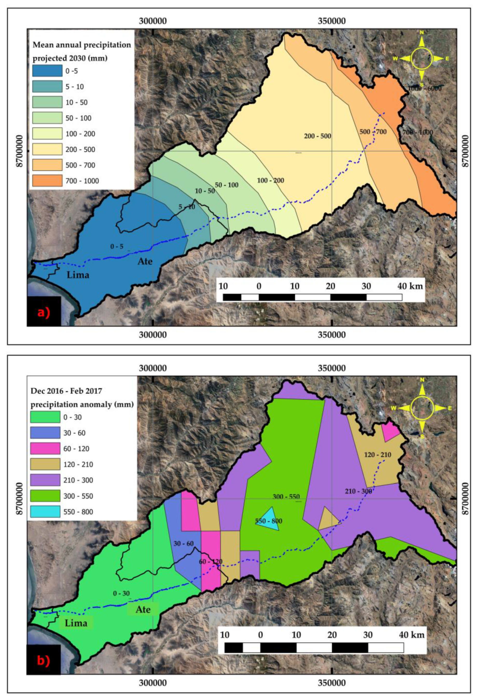
Precipitation in the coastal part of the basin is one of the lowest in the whole South America, with an average of 5 mm of accumulated annual rainfall [55] (Figure 3a). However, the air in the city is relatively humid, due to frequent haze and strong dew. Differently, at elevations higher than 1000 m above sea level, i.e., the medium-upper part of the Rímac River basin, the climatic conditions change to subtropical, dry desert climate, with accumulated annual values of precipitation equal to 750 mm [27,56]. This confirms that precipitation varies spatially across the basin depending on elevation, with the highest intensity upstream of the river basin, over the Cordillera of the Central Andes.
Accounting that at these latitudes the hydrological cycle runs from September to August, the heavy rain season falls between November and April. Such seasonal rains in the central highlands of Peru cause an increase in the water flow of the Rímac River compared to the other months of the year. This happened, for example, during the flood event in mid-March 2017. According to the regional hydrological warning of “red level” issued by the Servicio Nacional de Meteorología e Hidrología del Perú (SENHAMI) on the night of 17/03/2017, the maximum flow of the Rímac River was estimated to reach 95 to 100 m3/s, and 34 to 40 m3/s for the Chillón river, based on the measurements made at Chosica and Obrajillo hydrometer stations, respectively [57]. A precipitation anomaly with respect to mean historical records was indeed registered in the period December 2016–February 2017 (Figure 3b).
Throughout its history, the Rímac River has caused floods along its path many times, as a consequence of such seasonal rains. There are logs of this type of events since 1578 [58]. While these flood events are recurrent phenomena, when they occur in conjunction with ENSO, the Rímac River water flow exceptionally increases up to catastrophic level. Historically, 120 floods have been documented and association with ENSO has been reported [58], particularly in the years 1578, 1650, 1728, 1750, 1790, 1828, 1876, 1891, 1925, 1982, 1997, 2002, 2004, 2006, 2009, 2015, and 2017. With regard to the last hundred years, the chronological distribution of the flood events highlighted that there have been three periods of higher intensity in Peru, i.e., 1982–1983, 1997–1998 and 2017–2018 (Table 1). The direct relationship with the activation of ENSO events is so strongly believed that the whole period is referred to as “El Niño Extraordinario (i.e., the extraordinary El Niño event)” by scholars [8,9,11,21,26,59]. As already mentioned in Section 1, these events caused significant damage, hundreds of fatalities, and more than 2 million people were affected [29]. These recent events were selected as the focus of this investigation, since they are representative of the destructiveness that these hydro-meteorological events can bring. The satellite-based observations of the impact across the urban environment of Lima can therefore serve as an objective evidence of the areas at risk, if no hazard and risk mitigation measures are undertaken.

2.2. Synthetic Aperture Radar (SAR) Data Mining

The methodological workflow adopted, and main processing activities carried out can be divided into three components:
  • Processing of SAR satellite data and change detection products for image pairs.
  • Creation of a project catalogue (database).
  • Creation of the spatial analysis project on a GIS platform.

2.2.1. Selection of SAR Data

As mentioned in Section 2.1, SAR data were chosen for their independence from weather conditions and owing to their availability with a certain continuity with respect to the dates of occurrence of the flood events under study (see Table 1). Figure 4 shows the timeline of El Niño events vs. the whole archive of SAR data from the satellite missions ERS and ENVIronmental SATellite (ENVISAT) of the ESA, and the Copernicus Sentinel-1 constellation. These data are free and their access is unrestricted for registered users, through the open-source Earth Observation Link-ESA (EOLi-SA) for ERS-1/2 and ENVISAT (now via the ESA Online Dissemination tool), and the Copernicus Open Access Hub for Sentinel-1. As can be seen in Figure 4, of the most intense El Niño-related events, those occurred in 1982–1983 and 1987 could not be investigated since there were no SAR data available to cover those years. Furthermore, given that no ENVISAT data covered any of the other two El Niño-related events, these data were not used in the end.
Table 2 shows the main features of ERS-1/2 and Sentinel-1 data used for this research. The two ERS satellites, ERS-1 and ERS-2, were launched into the same orbit in 1991 and 1995 and ceased to collect data on 10/03/2000 and 05/09/2011, respectively [61]. Sentinel-1 is the SAR constellation made of the two twin satellites, Sentinel-1A (since 03/04/2014) and Sentinel-1B (since 25/04/2016), of the European Commission’s Copernicus programme, aiming to provide C-Band SAR data continuity following the retirement of ERS-2 and the end of the ENVISAT mission. Of the four acquisition modes of the Sentinel-1 SAR sensor, in this study we used the Interferometric Wide swath (IW) providing 5 m × 20 m (ground range by azimuth) resolution, over a 250 km swath [62].
Compared to the nominal satellite mission parameters reported in Table 2, it is worth noting that the number of ERS-1/2 images available over Lima and covering the entire Rímac River basin was less than expected, with revisit times sometimes higher than 35 days (i.e., 70 days at worst). On the other side, the ERS-1/2 mission was the only SAR data resource to investigate the 1997–1998 El Niño event. By contrast, the revisit time of Sentinel-1 data was almost regular, equal to 12 days as per the observation scenario over Peru in 2017–2018 [63]. Since the end of 2016, indeed, the programmed Sentinel-1 acquisitions over Peru account for a 12 days revisit frequency provided by the Sentinel-1B satellite only, with IW mode dual polarization data (Table 2).
In total, 39 images (13 ERS-1/2 and 26 Sentinel-1) were selected to investigate the flood events listed in Table 1, and were categorized into working pairs according to the following three groups: “Pre-event”, “Cross-event” and “Post-event” (Table 3). The full list of the working pairs is reported in the Appendix A (see Table A1, Table A2 and Table A3).

2.2.2. SAR Data Pre-Processing

The whole pre-processing activity, for both ERS-1/2 and Sentinel-1 images, was performed with the SentiNels Application Platform (SNAP) v6.0 software. The pre-processing allowed, for each image, the correction of orbit errors and/or geometric distortions, all of which were introduced during the acquisition of the SAR scenes. In particular, the pre-processing methodology included:
  • “Apply orbit file”: The orbit file (automatically downloaded by SNAP) provides an accurate position of the SAR image, and the updating of the original metadata of the SAR product.
  • “Radiometric Calibrate”: Calibration allows the creation of a SAR image where the value of each pixel is directly related to the radar backscatter of the surface, expressed in decibel (dB).
  • “Multilooking”: A characteristic of SAR images is the speckle, i.e., random noise that looks like a “salt and pepper” effect across the image, and affects the quality of the image, thus making SAR data interpretation more difficult. To remove such an effect, it is possible to use speckle filters or, alternatively, to multilook the image. A speckle filter is a compromise between speckle removal (radiometric resolution) and fine details preservation (spatial resolution). For Sentinel-1 images we applied “Multilooking” with 2 looks in azimuth by 2 looks in range [64]. For the ERS-1/2 images we applied “Speckle Filtering” using a Lee filter, which was selected among the possible filters to use according to the recommendations in [65], given that Lee filters are less degrading for the SAR image.
  • “Terrain Correction”: We converted the data from slant range geometry to the map geometry (UTM/WGS84 map projection) and corrected the main geometric distortions like layover, shadow and foreshortening, due to terrain relief, using the 3 arcsec Shuttle Radar Topography Mission (SRTM) [66] digital elevation model (DEM), as per the standard workflow of the SNAP software.

2.2.3. SAR Amplitude Change Detection

Change in the surface roughness is the key to detect inundation using SAR data. Where the ground surface is covered with calm water, its low roughness exhibits an almost ideal specular reflection and the backscatter is therefore very low (i.e., dark pixels in the SAR image), in strong contrast to the scattering of natural surfaces in dry conditions (i.e., bright pixels) [67].
The most straightforward way to detect surface changes between two dates/acquisitions is the comparison of the SAR radar backscatter. This approach is only sensitive to changes that impact the backscatter of the object, and does not take the entire complex SAR information (i.e., also the signal phase) into account [42]. Because floods alter the surface roughness, the change from dry to inundated conditions can be easily captured with SAR amplitude change detection. It is worth mentioning that this is the most common method for flood identification. Many studies have demonstrated that SAR systems are suitable tools for floodwater mapping on bare soil or scarcely vegetated areas where water has its well-defined radar backscattering signature.
However, there are some aspects that need to be accounted for when floods happen in densely built-up areas, and when medium resolution SAR images (such as ERS-1/2 and Sentinel-1) are used. In such environments, given the double bounce effect produced by buildings, and specular reflection of free-standing water, it may happen that flooded areas may exhibit stronger radar backscatter than the adjacent non-flooded areas [68,69]. A further factor influencing the intensity of the radar backscatter is the inundation depth vs. the height of the building. Depending on the extent of the building façade not flooded, double bounce may predominate over specular reflection.
Furthermore, it is known that, given the side-looking observation of space-borne SAR sensors, areas of urban ground surface may not be visible to the SAR due to radar shadowing and layover caused by buildings or taller vegetation and, therefore, urban flood extent may be not accurately detected [70]. These effects and interferences were taken into account during the interpretation of the change patterns, either increased or decreased radar backscatter, in the RGB composite and amplitude change detection maps that we generated for the periods 1997–1998 and 2017–2018.
In particular, the effects of local topography and the properties of the urban fabrics were considered based on the 30 m resolution Advanced Spaceborne Thermal Emission and Reflection Radiometer (ASTER) Global DEM (GDEM v.2) and urban land cover ancillary data (see Section 2.2.4). The following post-processing methodology for each SAR image pair listed in Table 3, Table A1, Table A2 and Table A3 was applied according to the workflow described in [41]:
  • “Coregistration stack”: which allows to overlay two images (input), i.e., the reference (master) and the secondary (slave), in order to ensure a perfect match between the pixels of the slave onto the geometry of the master reaching sub-pixel accuracy and, at the same time, preserving the original information contained in the slave [71].
  • “RGB Composite”: a multi-channel image generation, allowing for an immediate visualization of the changes in radar backscatter that occurred on the ground during the analysis period between the master and one or more slaves. Each of the R (red), G (green) or B (blue) channels (RGB) is allocated to either the master or the coregistered slave according to a specific combination of colors, thus obtaining a composite image where the different colors highlight different features. The assignment of the three RGB colors to the bands can be freely chosen. For this study, the assigned color scheme was as follows: R = master; G = slave; B = slave. When the slave is the same in both G and B channels, the RGB is actually a red-cyan (RC) composite. This choice allowed us to identify the changes due to the decrease in the backscatter signal in red (Figure 5a), while the changes due to the increase in the backscatter signal in cyan (Figure 5c).
  • “Ratio”: through a subtraction operation between bands of the slave image and the master image (values in both expressed in dB; see Section 2.2.2), the ratio map highlights any areas where changes in the backscatter radar occurred. The output of this operation is in grayscale, which, however, can be replaced by a freely chosen combination of colors for better viewing. The decrease or increase of the backscatter signal is displayed with dark colors (Figure 5b) and light colors (Figure 5d), respectively.
While the RGB/RC composites provide information on “where” the change occurred, the ratio maps provide information on the magnitude of such changes. These two outputs were the basis to identify the change patterns that have occurred in the Rímac River Basin and could inform about either the extent of floods or presence of urban changes (e.g., new residential areas) that were relevant due to their potential impact on local susceptibility to flooding.

2.2.4. Ancillary Data

The geospatial ancillary data (either vector or raster) related to topography, geology, permanent and seasonal water bodies, urban footprint, new urban development, roads and infrastructures, population at the district level, allowed us to access environmental and contextual information, gain more understanding and achieve a reliable interpretation of the radar backscatter changes that took place in the territory in 1997–1998 and 2017–2018. The details of the ancillary data are reported in Table 4. Data were handled, intersected and geospatially analyzed to a common coordinate system in the Quantum GIS (QGIS) platform (v. 3.2.3).
One Sentinel-2 cloud-free image was used as the optical basemap of the study area, to browse and consult alternatively to the cache-file Google Earth basemap, to find a first visual correspondence with the objects and shapes visible in the SAR images.
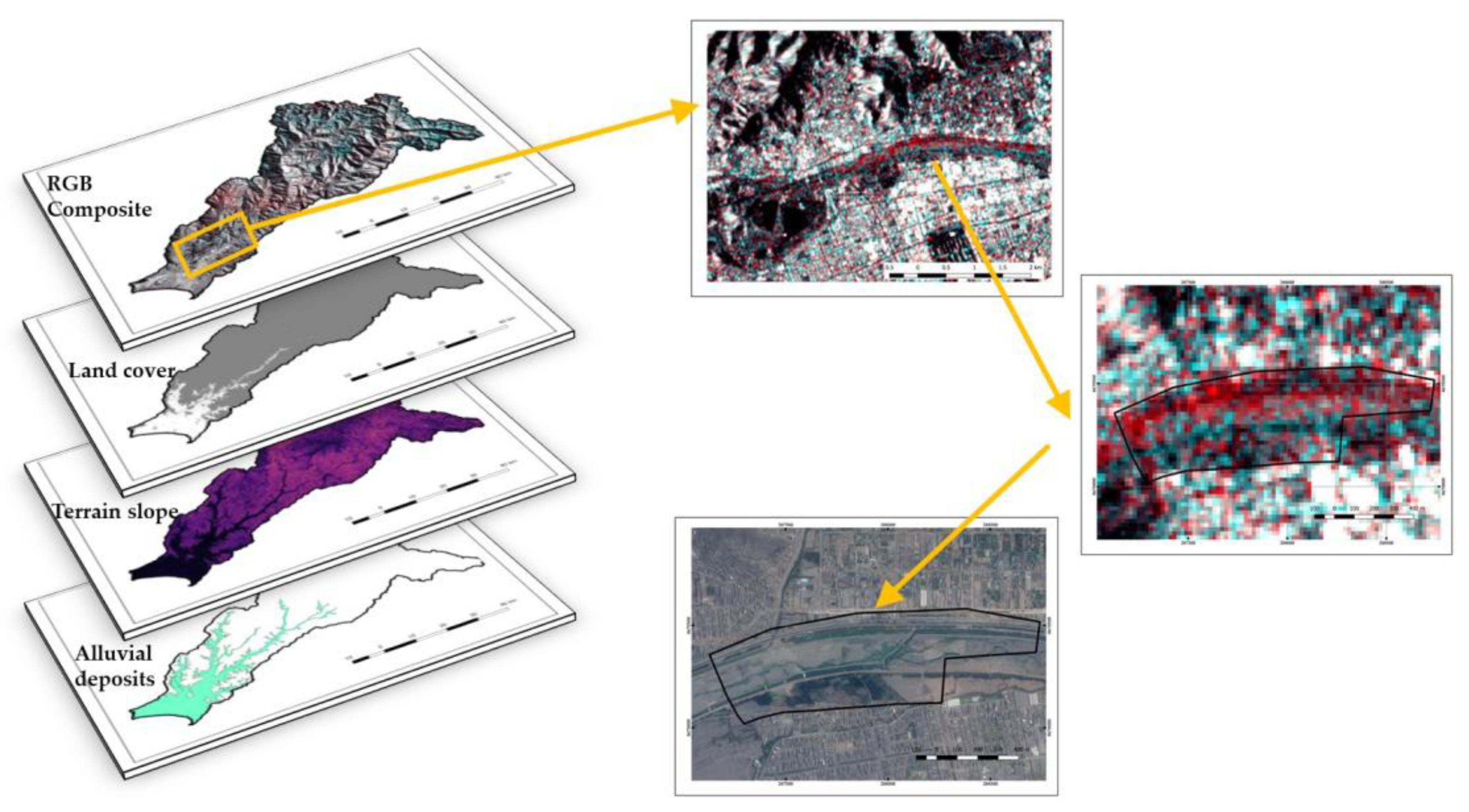
Figure 6 shows the three key spatial hazard datasets and risk elements that we examined to assess the hydraulic risk in Lima:
  • Terrain slope: this is a physical environment factor that contributes to the geological hazard as the predisposition of the territory to being flooded during a flood event depending on its elevation vs. the inundation depth. Initially, given that SRTM was used for the terrain correction of the SAR data (see Section 2.2.2), both versions of the same dataset, i.e., SRTM 1 arc-second (30 m) and 3 arc-seconds (90 m), were tested. However, they were replaced with the ASTER GDEM, given the evidence that the SRTM products were affected by gaps in some areas of the Rímac River basin and, as such, they were discontinuous and lacking information. Using the ASTER GDEM, instead, a raster was obtained, with slope values β ranging between 0° and 89°, and subsequently reclassified according to the following classes defined by 5-degree wide intervals: A: β ≤ 5°, B: 5° < β ≤ 10°, C: 10° < β ≤ 15°, D: 15° < β ≤ 20°, E: β > 20°, and finally vectorized. Class A, in particular, includes the alluvial terraces as per the classification in [82]. Alongside terrain slope, the ASTER GDEM has been used to characterize the (geo-)morphology and topography of the areas of interest, and to derive a comprehensive understanding of the physical characteristics that may make those areas prone to flooding, as per the standard practice in flood-risk research (e.g., [83,84]). This analysis has been embedded in the interpretation process of the observed change patterns (see Section 2.3).
  • Alluvial deposits: the material deposited or cemented into the lithological unit filling the fluvial valley is the geological factor that testifies a historical predisposition of the territory to alluvial events. The extent of alluvial deposits marks the lowlands of Lima and areas at the highest hazard for inundation.
  • Land cover: anthropogenic factor that indicates the spatial distribution and extent of the elements (e.g., houses, infrastructure) potentially exposed to risk. For this study, this layer mostly matches with the extent of the built-up areas and it was compiled by combining the information available through the Open Street Map (OSM) accessed from the QGIS service and the Global Urban Footprint (GUF) produced by the German Aerospace Center (DLR) with TerraSAR-X data [74,75]. Because these two datasets were updated until 2011, the OSM-GUF raster was complemented with new urban areas built between 2011 and 2019 that were digitized from Google Earth imagery.
The shapefiles obtained from the aforementioned three datasets (Figure 6) were integrated in QGIS, with the aim of producing basic thematic mapping (BTM) containing all the elements of hazard and risk elements that were used, alongside the SAR change patterns, to generate the final flood risk scenario map.

2.3. Hazard and Risk Analysis

The underlying concept behind this research is that the changes in SAR amplitude that we see in the compared SAR pairs can inform us about changes due to either transformations in the urban environment (e.g., new residential areas; terrain flattening; embankment) that could have contributed to increase or decrease one of the factors composing the risk equation (i.e., Hazard × Vulnerability × Elements at Risk), or impact of past floods. However, as it is well known in the literature, change detection techniques show where and when the SAR backscatter changed, and if it increased or decreased, but do not tell per se the reason that caused such change [41,85,86]. Furthermore, two SAR backscatter change patterns of similar magnitude and shape, either spatially close or distant, may be due to different processes. To this purpose, a process of interpretation of the observed SAR amplitude change patterns is needed.
In this regard, the brightness of features in a SAR image depends on the portion of the transmitted energy that is returned to the radar from targets on the surface. The magnitude or intensity of this backscattered energy depends on how the radar signal interacts with the surface, which in turn is a function of several variables or parameters. These parameters include the particular characteristics of the radar system (frequency, polarization, viewing geometry, etc.) as well as the characteristics of the surface (land cover type, topographic relief, etc.). Because many of these characteristics are interrelated, they cannot easily be separated into their individual contributions. The change in the various parameters may have an impact on, and affect the response of other parameters, which together affect the amount of backscatter [87].
SAR amplitude change patterns visible in the RGB composites and ratio colored maps (see Section 2.2.3) were extracted and delimited. This first skimming, however, did not allow us to give an accurate classification of the types of changes detected. For this purpose, a visual comparison with other sources like the optical basemap was necessary to ascertain the kind of changes that occurred. The changes were divided into two groups: “Flooding” if they could be attributed to issues of flooding; and “No flooding” if the changes were not related to flooding but could influence in some way the local susceptibility to flooding (e.g., motorway construction, landfill–earthworks, new building constructions; see Figure 6).
In this regard, such relevance was assessed based on the spatial intersection, in QGIS, between these changes and the factors (either anthropogenic or natural) as represented spatially by the vector and raster ancillary data described in Section 2.2.4 (Table 4). Therefore, for example, if a new residential area was found on alluvial deposits at low altitude, at closer distance from the Rímac River, this change was considered as “negative” in the overall risk equation because, at equal hazard and vulnerability conditions, it represents an increase of the local elements at risk. Vice versa, the construction of an embankment to protect residential buildings was considered as “positive” because, at equal vulnerability conditions and elements at risk, it contributes to decrease the local hazard to inundation. Furthermore, areas where no changes were found, but the processed SAR pairs showed evidence of flooding during previous events, were considered at risk and this information was translated into the high risk level of the final flooding risk map at basin scale.
The spatial integration with the ancillary data was also helpful to remove false positives, i.e., SAR backscatter changes that were not due to flooding. For example, permanent and seasonal water bodies (either natural or anthropogenic, e.g., water treatment plants The Atarjea and Planta de tratamiento de agua residual-PTAR Carapongo, as well as the reservoirs in Refineria Cajamarquilla), that could have been mistakenly interpreted as flooded areas in the cross-event pairs, were masked out and removed during the interpretation workflow, based on the externally validated ancillary data listed in Table 4 (e.g., Global Surface Water). Further verification of the correct identification of water bodies via this approach was achieved by comparison with the signals and SAR backscatter patterns found in the pre-event pairs, wherein the extent of water bodies was well visible and could not be confused with signals due to flooding.
The geospatial comparison in QGIS between the RGB and ratio maps from the different SAR image pairs covering all the three periods—i.e., pre-, cross- and post-event—was also exploited to ascertain where change patterns observed in the cross-event were due to increased soil moisture or wetting, and not to flooding. Furthermore, verification with coeval very high-resolution optical satellite imagery was made when available, such as for the March 2017 event (see Section 3.1.1). In this regard, it is worth noting that very few were the situations for which this check was necessary. As outlined in the description of the geomorphology of the study area (see Section 2.1), floodplains are very localized. Where present, they are either densely urbanized (therefore, no signal from soil moisture can be retrieved) or, if bare, are located at a distance from the river course and at an elevation that makes flooding quite unlikely, and (near-)surface wetting more plausible. In other situations (see Section 3.1.2), the precise delineation and geolocation of the observed SAR change patterns confirmed that the bare ground near the river course was not wet, or the soil moisture increase did not reach levels that could be seen at C-band.

3. Results

3.1. Flooding

A total of 197 changes attributed to the “Flooding” (F) group were highlighted, for a total of 32.10 km2. These changes are distributed throughout the whole extent of the riverbed of the Rímac River and, as expected, also include the areas that have been affected by the flooding events occurred in the years 1997–1998 and 2017–2018.
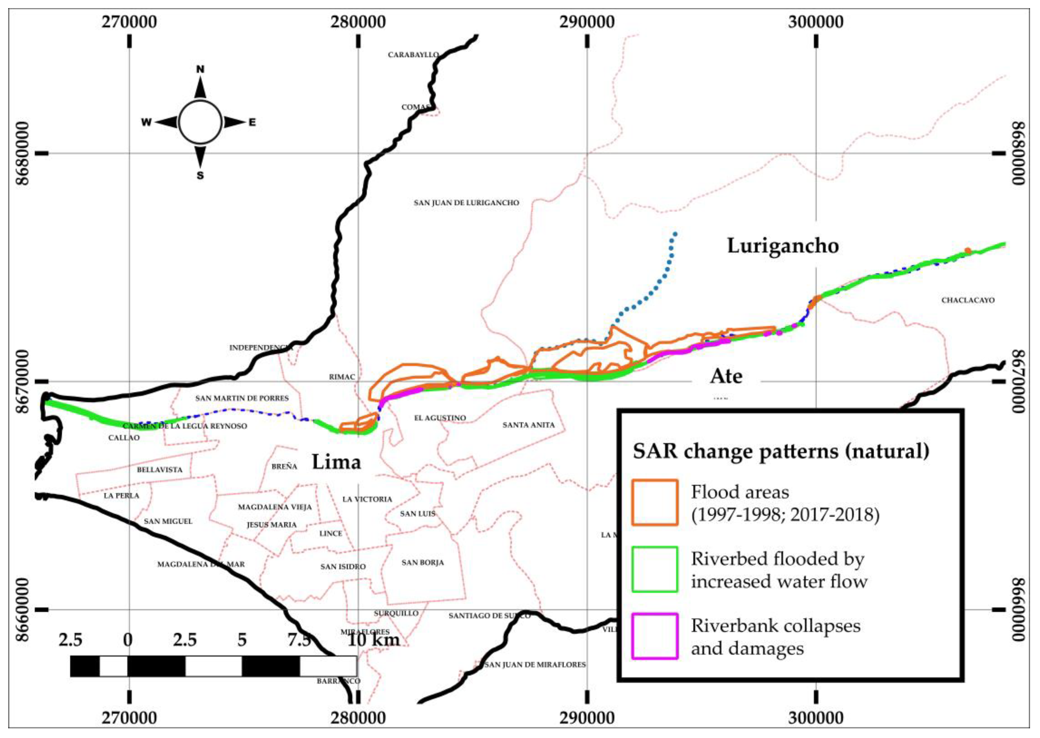
The 197 changes identified in the study area were delimited by the use of polygons, which were divided into three categories described in Table 5. Their spatial distribution is shown in Figure 7.
In the following sections, change patterns are discussed and interpreted according to the above categorization. For convenience and to avoid redundancies in figure legends, the same color coding is used for all the RGB composites and ratio maps presented hereinafter, according to the representation scheme described in Figure 5. Each figure is aimed to show a specific pattern, and not to be comprehensive of all the SAR backscatter change patterns displayed in the whole extent of the figure. Therefore, it should not be assumed that the neighbouring patterns were not interpreted, were excluded arbitrarily, or were not considered as relevant changes despite their similarity of appearance with the pattern that is highlighted in the figure and is commented in the respective caption.

3.1.1. Flooded Areas

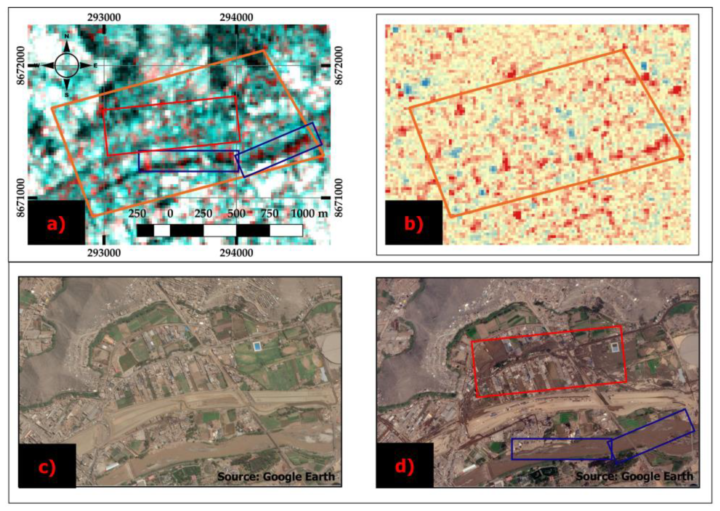
The F1 polygons concentrate mainly in the district of Lurigancho-Chosica. This is mainly due to the large residential and commercial areas that were flooded in mid-2017. In particular, Figure 8 shows the quarter in Carapongo lying on the right bank of the Rímac River, east of Av. Las Torres that runs along the bridge crossing the river not far from the Cascada de Huachipa. The RGB composite (Figure 8a) shows patterns of cyan color in correspondence with the area affected by the flooding event. Consequently, in that area the ratio map shows an increase of radar backscatter (Figure 8b). This outcome can be explained accounting that floodwater was not clear water, but rather contained solid material transported by the strength of the water flow. Field photographs published in the media show that, alongside wide flooded areas, there were several areas with debris accumulation, rubble, uprooted trees, damaged cars and heavy vehicles. This has also likely contributed to increase both the surface roughness and the soil moisture locally and, therefore, increase the radar backscatter.
This interpretation is also corroborated by comparing two very-high resolution optical images taken on 22/02/2017 (pre-event; Figure 8c) and 21/03/2017 (post-event; Figure 8d) and accessed through Google Earth. It is evident that the roads of the whole quarter were particularly muddy due to inundation. Furthermore, the careful inspection of the photographs capturing the Carapongo area mentioned above suggests that the effect of double-bounce backscattering resulting from the combination of inundation depth and the local urban layout, typology, geometry of buildings and road networks, may have contributed to the observed increase of radar backscatter. As recalled in Section 2.2.3, this complies with the SAR imaging theory in flooded anthropogenic environments, where the inundation depth and the height of the non-flooded portion of the building are sufficient to create the dihedral conditions for backscattering [68,69].
It is worth noting that all the 15 F1 changes were found on alluvial deposits and within urban areas. Of these areas, those closest to the riverbank have a B-class slope (5° < β ≤ 10°), while some of those that are more distant (500 m) are located on a D-class slope (15° < β ≤ 20°). Therefore, the satellite evidence that these areas were flooded confirms the local susceptibility to this hazard, as expected for areas located in lowlands and the alluvial valley.

3.1.2. Riverbed Flooded by Increased Water Flow

A total of 175 F2 type changes were identified, and they were all located within the riverbed. As per the example in Figure 9, these changes show a decrease in the radar signal due to the increase in the water flow and rise in the water level within the river, and typically occurred in correspondence with the transition from the dry to the rainy season (e.g., between December 2016 and March 2017). While these changes have a relative relevance for the flooding hazard itself (they occur in non-urban areas, in A-class slopes, i.e., β ≤ 5°), and are a typical consequence of the rainfall events and water excess, they are important to mark the sections of the river course where waters rise but, depending on the height of the riverbanks, may flow out and inundate the surrounding land, or not.
In this regard, it is worth noting the absence of change patterns along the long section of the urban canyon flowing between El Ejército Bridge in the district of Lima, and Universitaria Bridge in the district of San Martín de Porres (see the visible sections of the dashed line in Figure 7). There, the river flows across a canyon-like morphology, and is flanked by very high and steep banks (see Figure 1f), so any water flow excess is accommodated within the channel, and inundation is very unlikely.

3.1.3. Riverbank Collapses and Damage

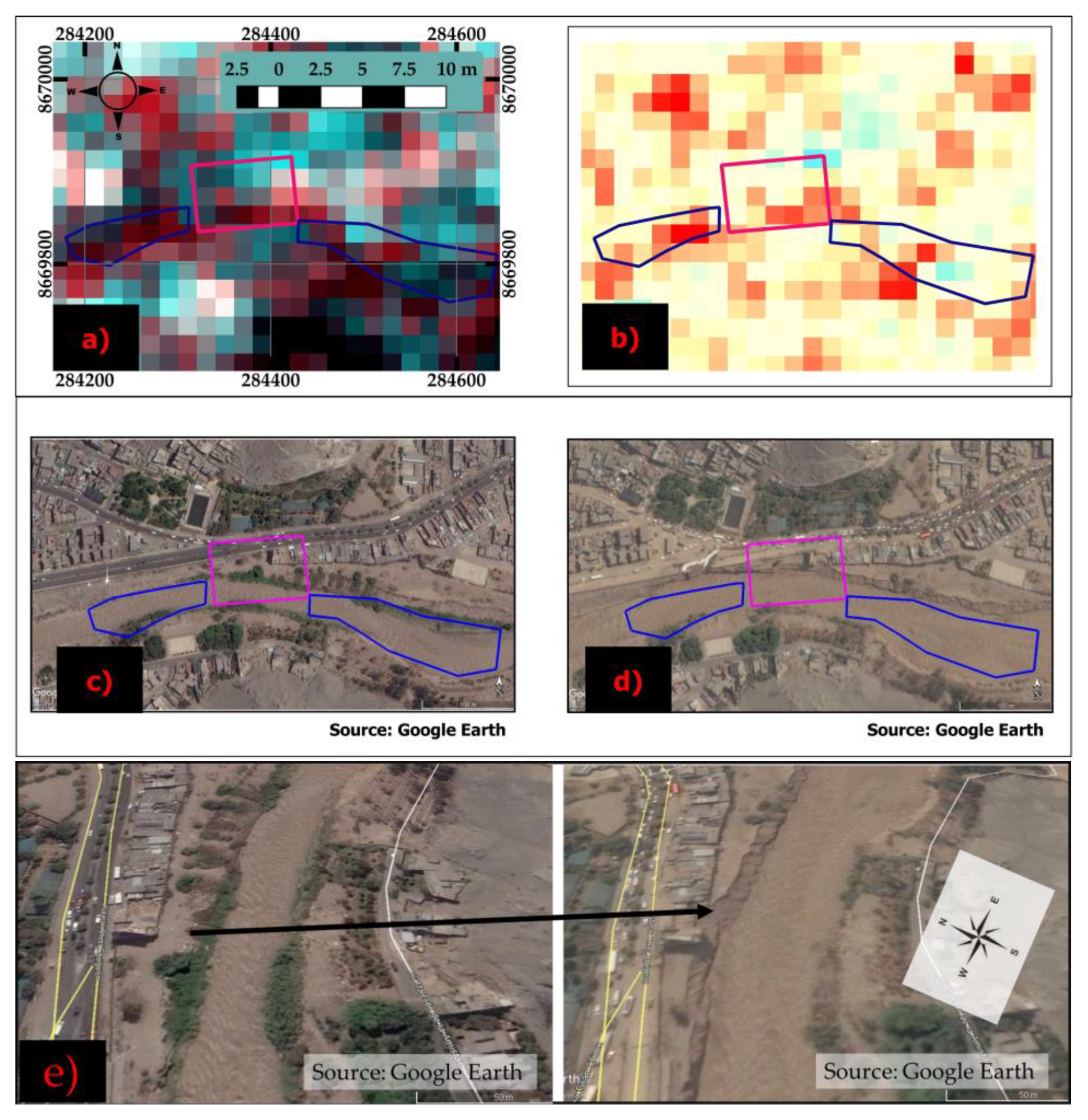
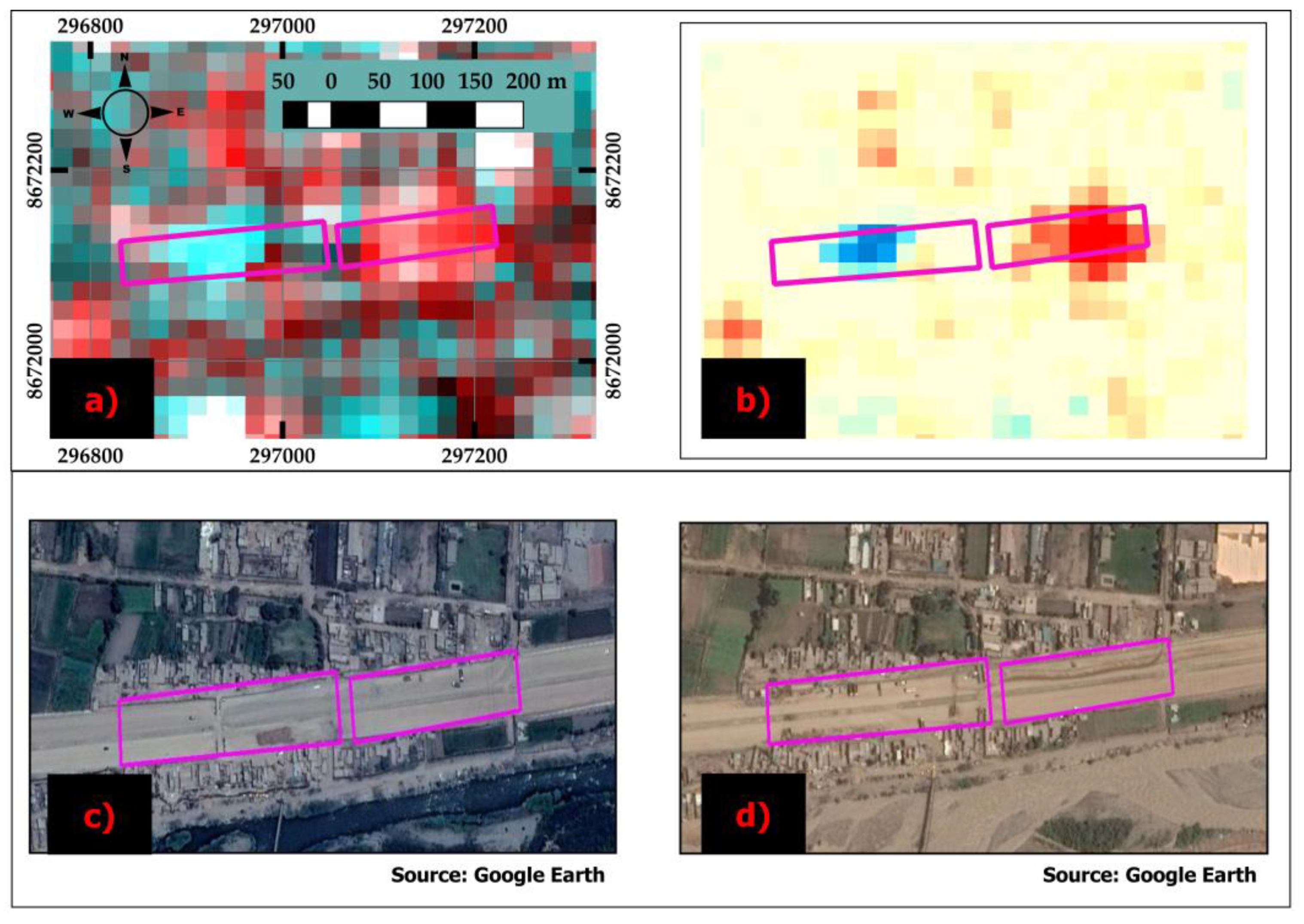
Cross-event SAR pairs also allowed us to capture seven radar backscatter changes (i.e., decrease) due to collapses of some sections of the riverbank that, in some cases, have also caused damage to critical infrastructure (e.g., bridges). They are located on alluvial deposits, near urban areas and with an A-class slope (β ≤ 5°). Figure 10 shows the example of an area, in the district of Lurigancho-Chosica at the intersection of Malecón Checa Eguiguren and Gran Chimú avenues, that has lost material due to the increase in the Rímac River water flow and the collapse of part of the riverbank. The post-event Google Earth image shows the detachment niche of the riverbank collapse and the new scarp cutting one of the buildings (Figure 10c–e) and making the stability of the neighboring houses quite precarious.
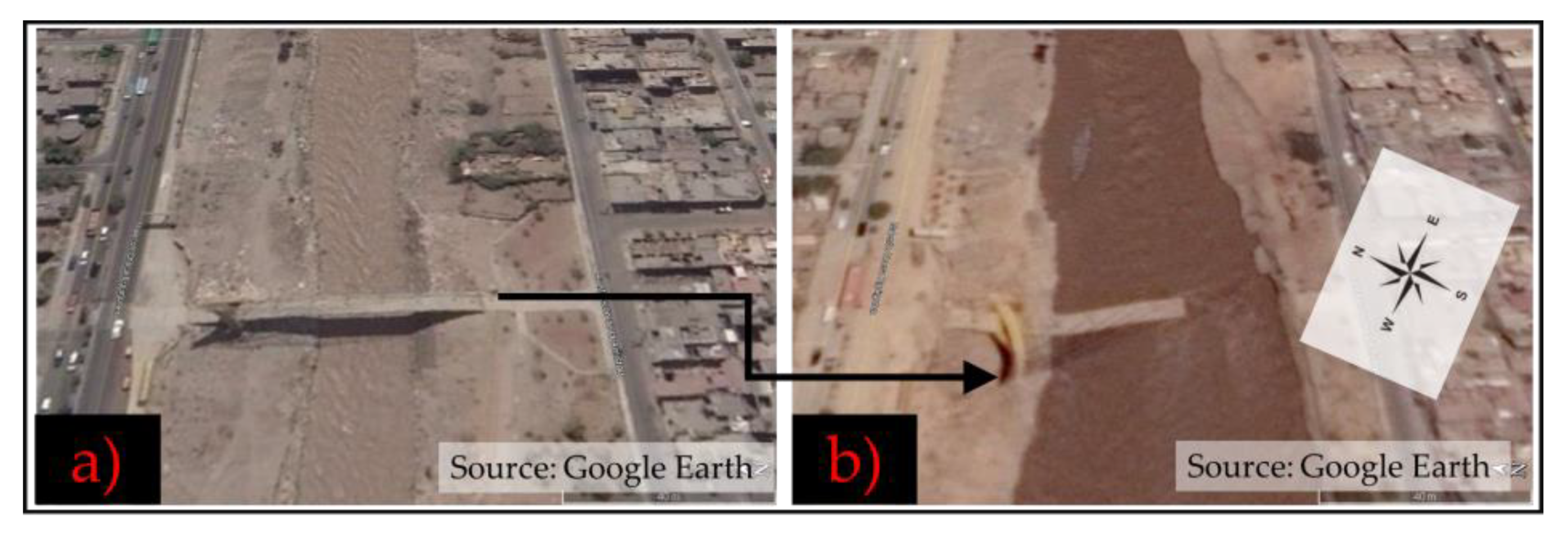
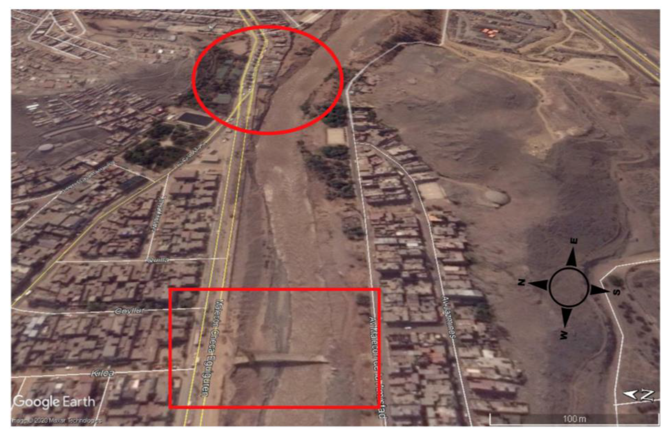
Another example was found in the Talavera Bridge, in San Juan de Lurigancho. As also documented in a video published online [88], the part of the bridge collapsed down into the river water during the flood event occurred on 16/03/2017 (Figure 11 and Figure 12). This bridge had been built only six and a half years before.

3.2. No Flooding

The changes related to anthropogenic activities (hereafter named “No flooding”, NF) that occurred in relation to the periods 1997–1998 and 2017–2018 and were identified in the 39 working SAR pairs, are 212 in total (26.40 km2). These are distributed throughout the Rímac River basin area, and many of these changes are due to new urban settlements, growth in trade activities, and development of new roads.
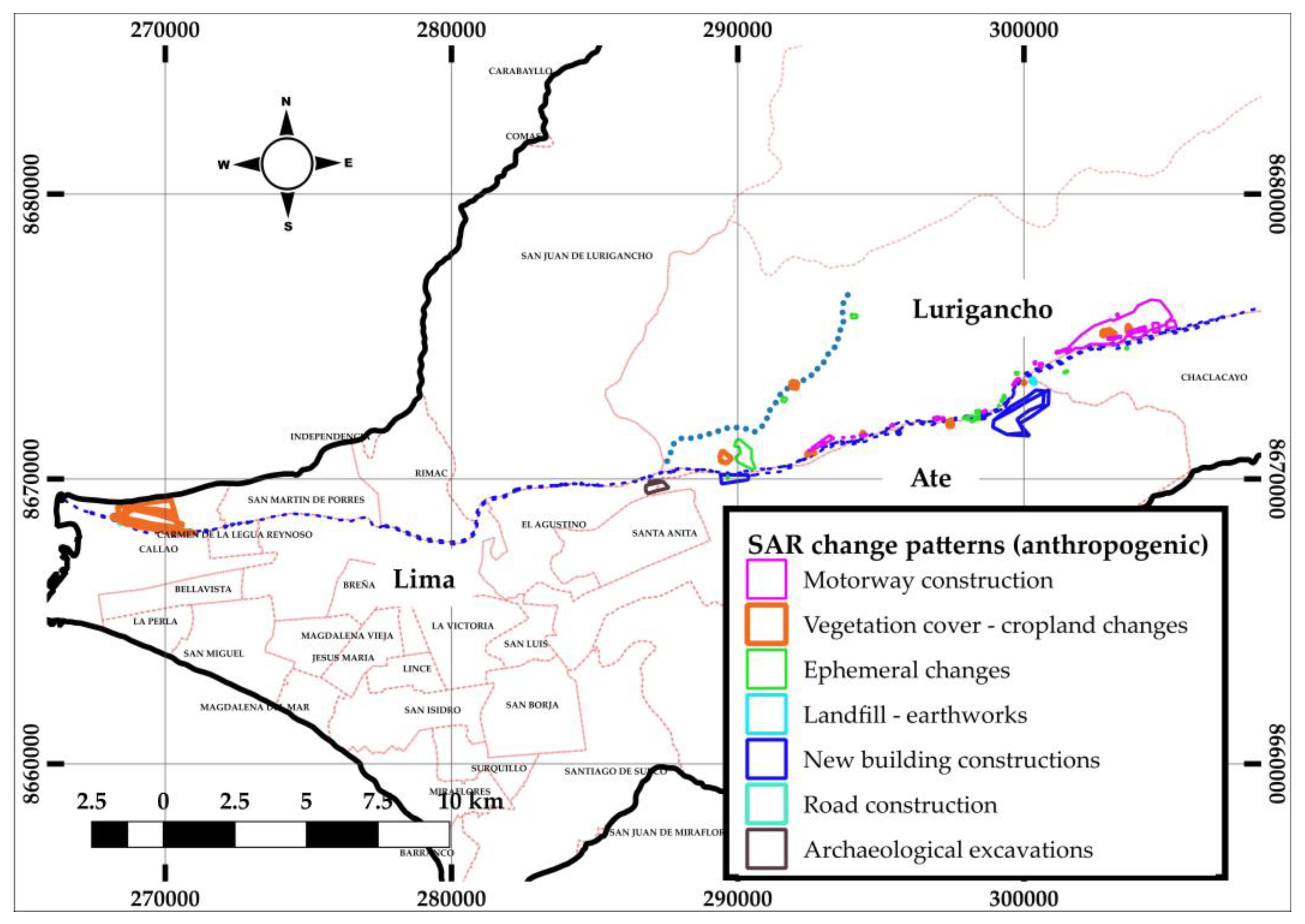
Changes related to anthropogenic activities have been divided into 13 categories, which are described in Table 6. Figure 13 shows the distribution of the areas in which changes in the radar backscatter have been observed as a consequence of anthropogenic activities (i.e., categories NF1, NF2, NF3, NF7, NF9, NF12, and NF13).
To assess the risk of flooding:
  • Changes due to anthropogenic factors falling within the categories NF1, NF3, and NF13, were all considered because of their spatial position with respect to the hazard factors (natural, geological and anthropogenic) that could suggest a potential impact on increasing the risk locally;
  • Of the changes falling within the categories NF2, NF7, NF9, and NF12, we considered only those located in areas that were very likely to be affected by any future flooding events, given the local slope or because of their proximity to the Rímac River;
  • In contrast, categories NF4, NF5, NF6, NF8, NF10, and NF11, were not taken into consideration since they were changes not relevant for the hydraulic risk zoning.
The above criteria led us to select 82 out of the total 212 NF changes for the hydraulic risk interpretation. The key characteristics of the NF1, NF2, NF3, NF9, and NF13 changes can be summarized as follows:
  • Motorway construction: the 37 radar backscatter changes corresponding to the construction of the New Central Highway (NAC), show both increases and decreases in the radar signal, due to the movement of machinery, workers, landscaping, among others, thus resulting in a non-homogeneous signal backscatter (Figure 14). These changes are located on alluvial deposits, with slopes in A and B-class (23 and 14 changes, respectively), and in non-urbanized areas.
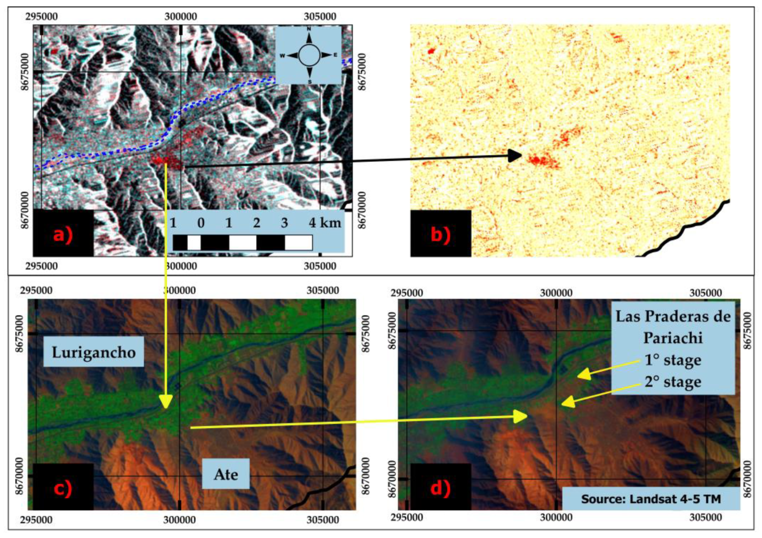
  • Vegetation cover–cropland changes: there are 18 changes, located in non-urban areas and on alluvial deposits, and with A-class slope (β ≤ 5°), due to growing crops or land use changes, e.g., transition to new residential/commercial buildings (Figure 15).
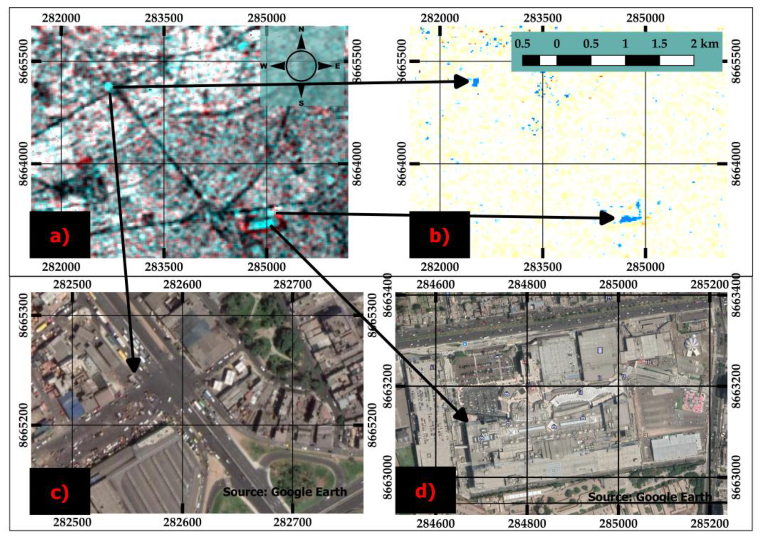
  • Ephemeral changes: increase in the radar backscatter was observed in 15 areas as a consequence of an increase in the number of vehicles parked (Figure 16). These changes are located on a slope between A and B-class, on alluvial deposits, with eight changes on non-urbanized areas, and the other seven on urban areas.
  • New building constructions: these five changes are considered important for risk assessment, since they have a low slope (A-class), and in conjunction with their proximity to the river, they match with elements that can be easily flooded. They are located on alluvial deposits, and in urban areas (Figure 16).
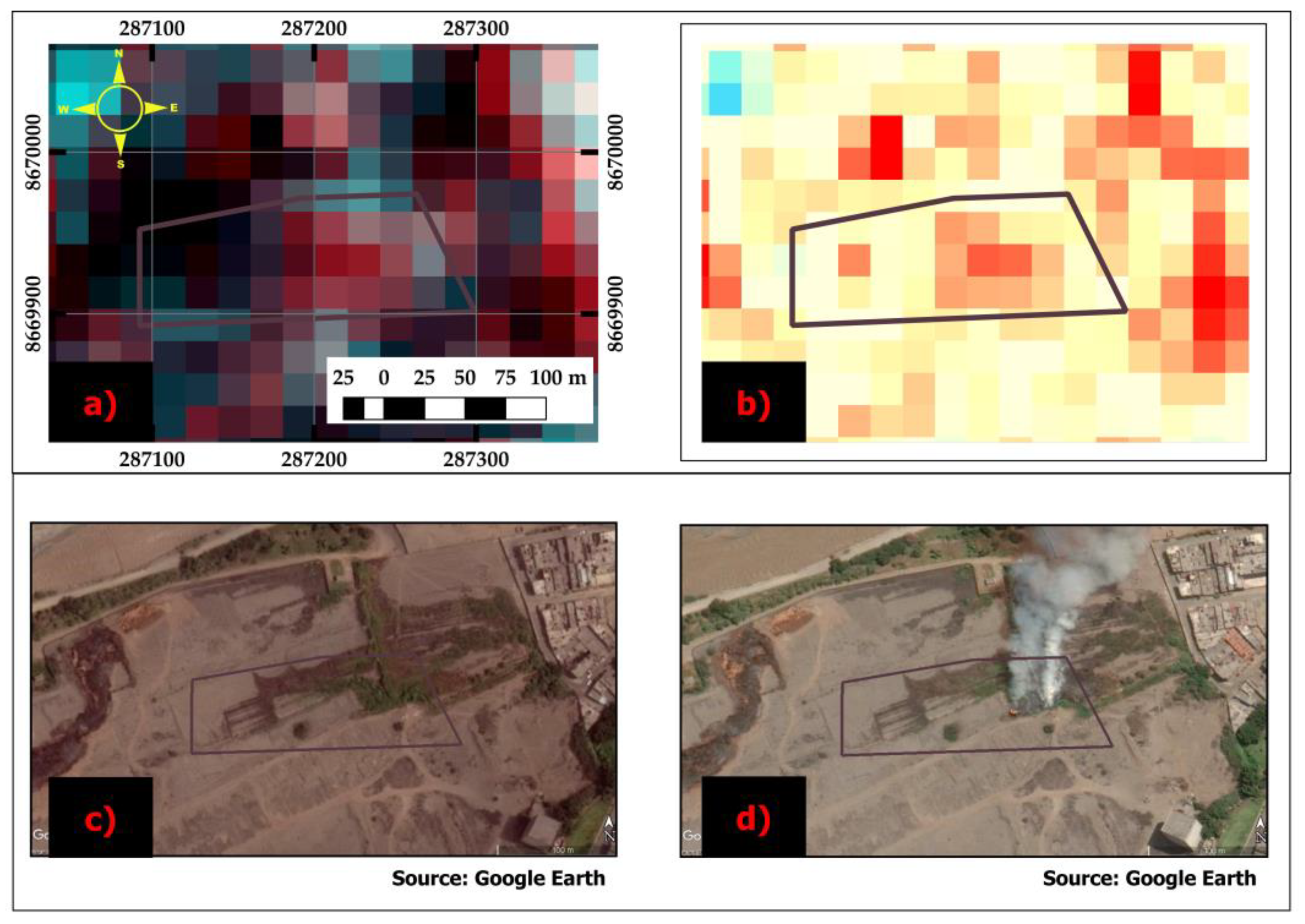
  • Archeological excavations: four changes in the radar backscatter show decrease in the signal in areas with archaeological remains. In one case, the decrease in the backscatter signal could be influenced by the decrease in vegetation in the archaeological area due to a fire (Figure 17). These changes are located on alluvial deposits, on a non-urban area with an A-class slope.

3.3. Zoning of Areas at Risk in Case of Events of Equal Severity

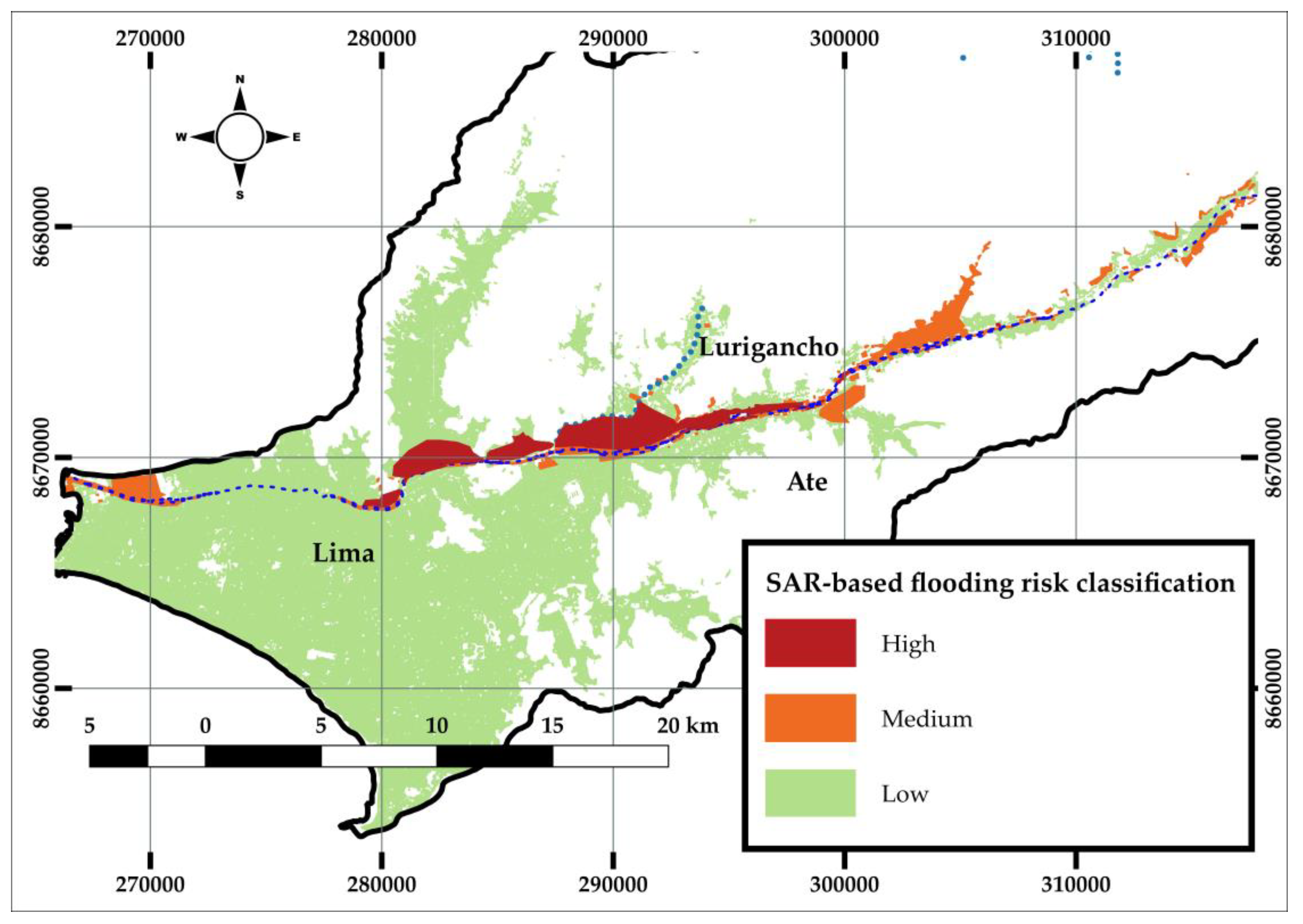
For the generation of the Rímac River basin flood risk map, three risk levels were defined: high, medium and low risk. The factors determining the level category were, first of all, the terrain slope, the surface occupied with alluvial deposits, and/or the presence of urban or non-urban area. For this reason, the characteristics of the changes taken into account for risk analysis are summarized in Table 7. At a glance, it can be noted that all the changes are located onto alluvial deposits, their most common slope class is A to B, and they split among urban and non-urban areas.
The areas identified at a high risk of flooding are those that in the years 1997–1998 and 2017–2018 were directly affected by the flooding event, and where satellite data and/or ground evidence suggest that material loss occurred (e.g., collapse of riverbanks), slope was classified as A or B, and urban fabric is onto alluvial deposits. Categories F1 and F3 correspond to this description, with a total of 22 changes and a total area of 19.44 km2.
The medium risk was attributed to non-urban areas that could be affected by flooding events as a result of the combination between slope class A to B and presence of alluvial deposits. The categories that correspond to this description are F2, NF1, NF2, NF3, and NF13. The medium risk classification was also applied to those urban areas, characterized by slope class A or B, and the presence of alluvial deposits, that changed during the studied period and that due to their proximity to the Rímac River could be affected by flooding events (i.e., change categories NF7, NF9, and NF12).
In the end, urban areas where neither previous evidence of flooding nor changes in the satellite data were found, and where it is very unlikely that they would be inundated due to their slope characteristics (up to D) and/or local geology, were classified at low risk. A total of 158 polygons of the newly identified urban areas fall within this category (15.54 km2).
Figure 18 shows the obtained risk map for the hydrographic basin of the Rímac River and city of Lima. Because this map is the outcome of combining hazard and risk factors (i.e., via analysis of the BTM), and the changes (both due to flooding or not) found in the SAR data, it provides the zoning of the areas at risk with respect to flooding events of equal or greater magnitude than those occurred in 1997–1998 and 2017–2018, if no hazard and risk mitigation measures are undertaken.

4. Discussion

In its history, Lima has experienced many flooding events. In the last few years many cartographic mapping efforts have been conducted to identify the areas affected by these events. These mapping exercises were made in-situ, with field inspections, or with the aid of satellite and aerial optical images (e.g., [28]). The studies published by [33,34] were the first to approach the use of SAR data, and aimed to highlight areas affected by landslides and flooded in the city of Chosica, located 60 km from Lima in the mid-upper part of the Rímac River basin.
Based on the current state-of-the-art on these events (see also Section 1), our study is the first that attempts the hydraulic risk mapping for the urban areas of the Rímac River basin, with the use of satellite SAR data. The risk mapping obtained as a result of the change detection methodology has demonstrated the ability of this approach to extract valuable information relating to the changes that have developed in the territory over time. This methodology has been very useful in analyzing changes due to flooding and other types of processes (here called “No Flooding”, NF), especially in an area like the Rímac River basin that is characterized by sudden geomorphological changes (from one year to the next), due to the severity of geodynamic phenomena occurring along the Rímac River tributaries.
RGB color composites and ratio maps mutually complemented in enhancing the areas of the basin where changes have occurred, through patterns of decrease vs. increase of the radar backscatter. As recalled in Section 1, from an analytical point of view, this is the practical advantage of this change detection approach compared to other more sophisticated methods.
To assess the accuracy of this approach in detecting changes due to flooding, we have compared our results with the map product that was generated by the Copernicus Emergency Management Service (EMS) during the Risk and Recovery Activation EMSN-038 for flood delineation and damage mapping of the flooding event that happened in mid-March 2017 [44]. The activation was under the Framework Service Contract No. 259811 (“Emergency Management Service – Risk and Recovery Mapping”) and, alongside optical satellite images, the same Sentinel-1 ascending (17/03/2017) and descending (18/03/2017 and 24/03/2017) mode images were used for flood detection. The mapping team reached similar conclusions as in our study, i.e., that the traditional approach based on detecting the decrease of radar backscattering and combined thresholding/region-growing could not work, given the characteristics of the urban environment in Lima, as well as the character, timeline and extent of the flood event [44]. For this reason, a change detection approach was employed for the EMS activation, using the shortest available temporal baselines (i.e., 12 days for both tracks).
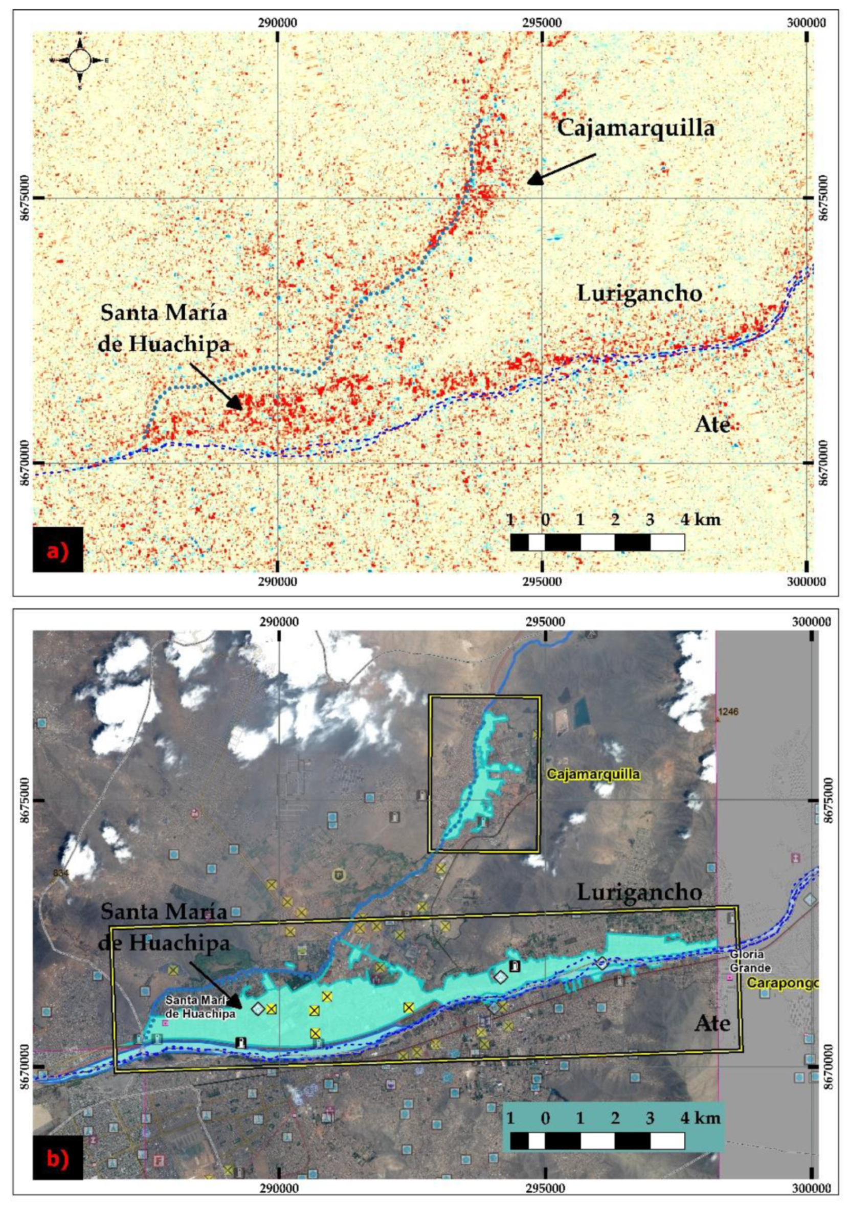
Figure 19 allows the spatial comparison between our ratio map (Figure 20a) and the EMSN-038 potential maximum flood extent (Figure 19b) in the area of Carapongo/Santa María de Huachipa and Cajamarquilla that were the first and second largest areas to be inundated, respectively. The two mapping products provide different, but complementary and interlinked information: while the EMS map focuses on those areas at potential maximum flood, our ratio map documents all the SAR backscatter changes captured in the cross-event pairs of the analyzed interval and, as such, shows many more changes. From the geospatial intersection between the two products, it comes out that the higher concentrations of SAR change patterns found for the 2017 flood event, and interpreted as due to inundation from the Rímac and Huaycoloro rivers, fall where the EMS spatial mapping delineated the most affected areas. Therefore, the change detection methodology based on SAR data provides a robust and validated input to the risk classification presented in this study (Figure 18). While the above comparison reassures about the accuracy of our change detection approach, the classification of the observed “Flooding” (F) and “No Flooding” (NF) changes could not have been achieved reliably without the image analyst interpretation of the patterns and magnitude of the changes in the radar backscatter based on the integration with the ancillary and BTM data. As such, given that flood products of international programs (e.g., Copernicus Emergency Services) exploit different image-based approaches for flood detection, the methodology presented in this paper could complement them, provide value-added and be disseminated in national and international disaster risk reduction/emergency mapping frameworks.
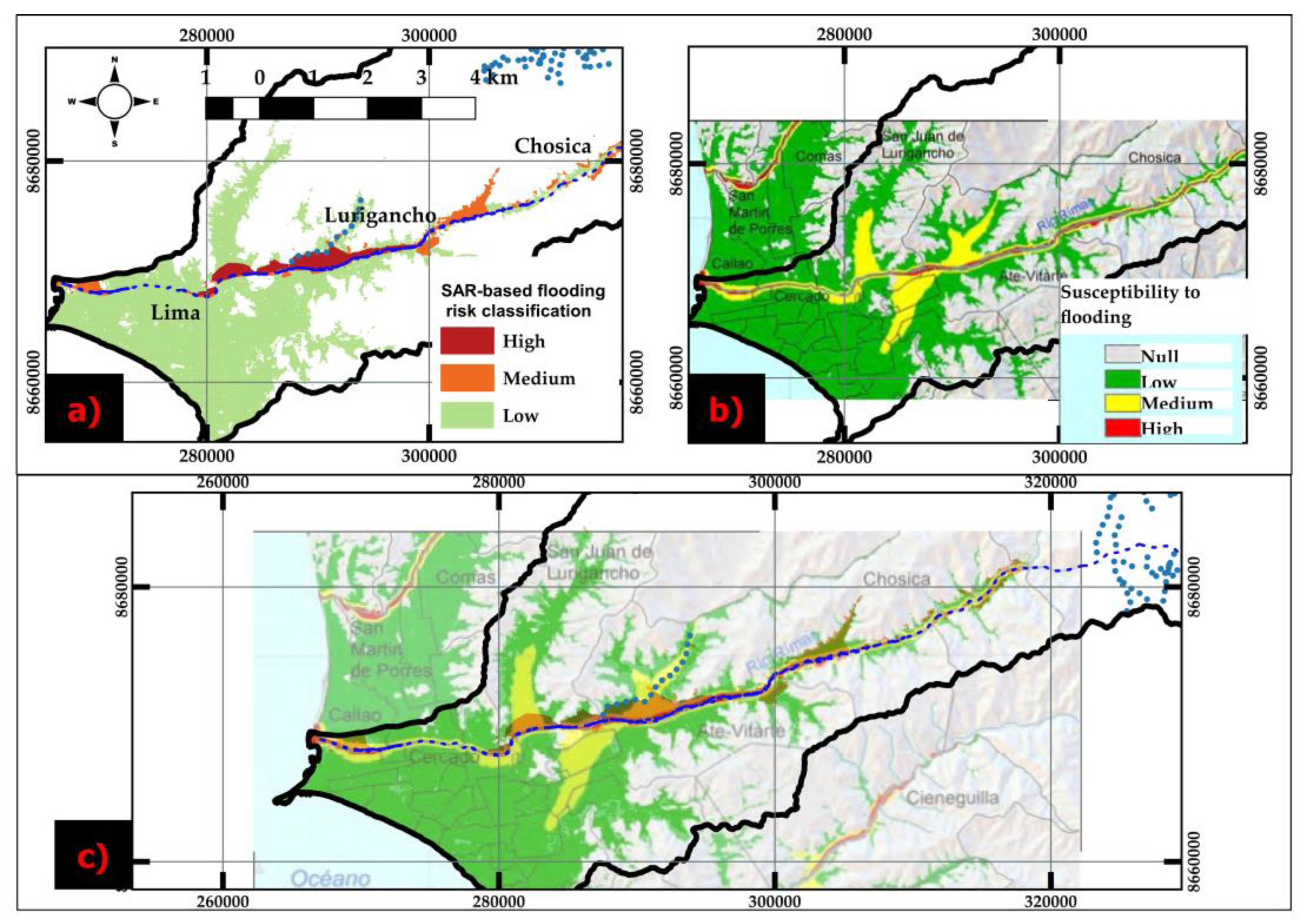
To assess the accuracy and reliability of our risk map (Figure 18), we compared it (Figure 20a) with the map of flooding susceptibility and fluvial erosion published by Villacorta et al. [28] (Figure 20b). Both maps have a very similar distribution for the areas classified as at low risk, while they show significant differences for the areas classified as at high and medium risk. In particular, two main differences exist. First, some areas that in Villacorta et al.’s map (Figure 20b) are identified as at medium risk, in our map are classified as at either low or high risk. Second, our map encompasses some larger areas at high risk along the river course that have been flooded. In the first case, it is very likely that the areas at higher risk classification in Villacorta et al.’s map reflect the availability of more granular and higher detailed geological and topographic information to assess the flooding susceptibility than the open data (that were accessed for this research) could provide. In the second case, it is clear that, the information derived from the SAR images emphasizes the areas that have been already flooded and/or where urban changes that may increase risk have occurred. Therefore, our risk classification map embeds event-based information and knowledge of the impacts of urbanization that allow the improvement of the hazard mapping made solely based on geological factors. Therefore, the observed difference between the two maps should not be interpreted as a discrepancy, but instead as an objective demonstration of the benefits that information mined from SAR time series can bring in to improve hazard mapping products, as well as the value of high resolution geospatial information in flood hazard mapping.
By knowing the temporal variability of the flooding events, it is possible to understand their impact at the basin, public safety and urban infrastructure level. If produced on a regular basis, such SAR-based mapping of urban and environmental changes would be a key instrument of disaster prevention. Early identification of areas potentially at risk of flooding is a prerequisite for the preparation of effective risk prevention and/or mitigation measures, with the effect of improving policies in the area, and consequently paving the way for the reduction of socio-economic impact that a flood would cause.
For the case study of Lima, it is worth noting that the hydraulic risk map presented here was developed a posteriori, since the flood events had already happened. Therefore, it embeds information that was captured from SAR satellites during past events. As such, it represents a zoning of the hydrological risk of the urban areas that have been affected by the flood events under study, and provides an indication of risk should events of similar magnitude affect Lima again in the future.
Some limitations were found during the study with regard to the following aspects:
  • The quality of archive satellite imagery available for the area was uneven. In addition to the ERS-1/2 scenes used for the analysis (see Section 2.2.1), 29 more ERS-1 images were downloaded from the EOLi-SA catalogue and pre-processed but, in the end, they could not be used due to issues affecting the raw data and their geolocation (due to Doppler Centroid values >2000 Hz), as reported by ESA’s EO Help team. These images were not included in the input dataset catalogue, and therefore the amount of archive data that could be incorporated in the change detection analysis was reduced.
  • Information gaps (missing values) were found in the DEM obtained by the Shuttle Radar Topography Mission (SRTM; see Section 2.2.4). For the case of Lima, data from the ASTER Global DEM (GDEM v.2) was used to address this problem. Alternatively, to remedy the lack of information in the SRTM DEM, measurements taken directly in the field in areas of uncertainty, or by interpolation of level curves, could have been used, but this was outside the scope of the present research.
  • The lack of ancillary information with which to carry out a complete analysis. Specifically, the absence of updated information on urban land cover was a limit that had to be overcome at the beginning of this research by creating an ad hoc spatial layer through the union of data from the Global Urban Footprint (GUF) and manual digitization of new urban areas, the latter based on very high-resolution optical satellite images accessed through the basemap service of QGIS and Google Earth.
  • The nominal revisit time of the SAR satellites used for this study, i.e., 35 days for the ERS-1/2 and 12 days for the Sentinel-1 (because since October 2016 the area is surveyed by Sentinel-1B satellite only, according to the constellation observation scenario currently operating [63]), which did not allow for acquiring data on the specific days when the flood events occurred, or with shorter site revisits. However, the multi-temporal approach based on multiple pre-, cross- and post-event SAR pairs has increased the possibility of identifying changes relevant to the analysis.
  • Both natural and anthropogenic changes have been identified in the SAR images used for this study. Therefore, an expert-led interpretation operation was needed to correctly classify the observed changes into the different categories of “Flooding” (F) and “No Flooding” (NF) and, therefore, to identify the occurred variations in the urban fabric that had some relevance for the purposes of flood risk zoning.

5. Conclusions

The Rímac River basin in the city of Lima in Peru is susceptible to flooding as demonstrated by the history documented in the natural disaster catalogues, due to both its intrinsic hazard factors (natural, geological and anthropogenic) and geographic location, which together lead to greater exposure to hydro-meteorological events triggered by the El Niño.
The present study of the flooding events occurred in 1997–1998 and 2017–2018 demonstrates that the radar signal amplitude information extracted from ERS-1/2 and Sentinel-1 satellite SAR images can allow the identification of changes in the territory and, consequently, can be used as an objective information to improve the assessment of susceptibility to flooding hazard and corroborate what is known from in-situ observations and mapping of damage on the ground. By integrating the information mined from the SAR scenes with ancillary data on land cover, urbanized areas extent and geological information, the various sectors and zones of the Rímac River basin were classified in relation to the potential impact of flooding on the built environment and urban infrastructure, in light of the recent natural hazard events and urban development. Therefore, we developed a map of flooding risk classification at basin scale that, compared to existing hazard maps, has the advantage of using SAR data to enhance areas at high risk based on the evidence that they were already flooded during recent events, and warn about the consequent likelihood to be flooded again, should no risk mitigation measures have been put in place and events of equal severity occur in future.
The comparison with the official map product that was generated by the Copernicus EMS during the Risk and Recovery Activation EMSN-038 for flood delineation and damage mapping of the same flooding event that happened in mid-March 2017 proves the accuracy and reliability of our change detection method, and reassured us that it provides a robust and validated input to the risk classification.
The hydraulic risk mapping carried out in this study was developed a posteriori, that is, after the 1997–1998 and 2017–2018 flood events had already happened. However, the methodological approach presented in this paper can be applied in future for regular monitoring of the Rímac River basin, with the aim of updating the knowledge and understanding of flood risk factors and the consequent susceptibility. The SAR-based methodology is indeed suitable to be iteratively applied, should newly acquired SAR images be analyzed and/or other events occur. In this regard, it is worth recalling that such regular mapping of changes (either natural or anthropogenic) is a key element in the framework of disaster risk management, as it contributes to preparedness, resilience building and reduction of impacts of such natural hazard events on socio-economic levels.

Author Contributions

Conceptualization, D.T. and F.C.; methodology, N.A.R.; formal analysis, N.A.R.; resources, D.T. and F.C.; data curation, N.A.R.; writing—original draft preparation, N.A.R.; writing—review and editing, D.T. and F.C.; supervision, D.T. and F.C. All authors have read and agreed to the published version of the manuscript.

Funding

This research received no external funding.

Acknowledgments

This research was carried out during the internship of N. Alvan Romero at the Italian Space Agency (ASI) under the supervision of D. Tapete and F. Cigna, in the framework of the II Level Master in Space Science and Technology at the University of Rome Tor Vergata (Italy). Copernicus Sentinel-1 and Sentinel-2 data were sourced from the European Space Agency (ESA)’s Copernicus Open Access Hub, while ERS-1/2 data were accessed through EOLi-SA (project ID 45250). Google Earth images (© 2020 Maxar Technologies) were sourced and analyzed from Google Earth Pro. Global Urban Footprint (GUF) product over Lima was provided by the German Aerospace Center (DLR).

Conflicts of Interest

The authors declare no conflict of interest.

Appendix A

This appendix provides details of the ERS-1/2 and Sentinel-1 SAR image pairs used to study the flood events that occurred in Lima in 1997–1998 (Table A1) and 2017–2018 (Table A2 and Table A3).
Table A1. ERS-1/2 SAR image pairs analyzed to map the urban changes in 1996–1998 and assess the impact of the El Niño-related flooding events that occurred on 09/02/1998 and 23/02/1998.
TrackPre-EventCross-EventPost-Event
218-10/04/1996–20/05/199820/05/1998–29/07/1998
397-22/04/1996–01/06/199801/06/1998–19/10/1998
447-26/04/1996–01/05/199801/05/1998–14/08/1998
12503/04/1996–15/10/199715/10/1997–22/07/199822/07/1998–26/08/1998
Table A2. Sentinel-1 SAR image pairs analyzed to map the urban changes in 2016–2017 and assess the impact of the El Niño-related flooding events that occurred on 14/01/2017, 31/01/2017 and 16/03/2017. It is worth noting that in a few cases the same pair (e.g., 17/01/2017–10/02/2017) can be used as cross- and/or post-event in relation to the dates of the events.
Relative OrbitPre-EventCross-EventPost-Event
1830/11/2016–24/12/201624/12/2016–17/01/201717/01/2017–10/02/2017
24/12/2016–17/01/201717/01/2017–10/02/201710/02/2017–22/02/2017
22/02/2017–06/03/201706/03/2017–18/03/201718/03/2017–30/03/2017
17105/11/2016–29/11/201629/11/2016–16/01/201716/01/2017–09/02/2017
23/12/2016–16/01/201716/01/2017–09/02/201709/02/2017–05/03/2017
09/02/2017–05/03/201705/03/2017–17/03/201717/03/2017–29/03/2017
Table A3. Sentinel-1 SAR image pairs analyzed to map the urban changes in 2018 and assess the impact of the El Niño-related flooding events that occurred on 14/02/2018 and 22/02/2018. It is worth noting that in a few cases the same pair (e.g., 16/02/2018–28/02/2018) can be used as cross- and/or post-event in relation to the dates of the events.
Relative OrbitPre-EventCross-EventPost-Event
1824/01/2018–05/02/201805/02/2018–17/02/201817/02/2018–01/03/2018
05/02/2018–17/02/201817/02/2018–01/03/201801/03/2018–13/03/2018
17123/01/2018–04/02/201804/02/2018–16/02/201816/02/2018–28/02/2018
04/02/2018–16/02/201816/02/2018–28/02/201828/02/2018–12/03/2018

References

  1. IPCC. Intergovernmental Panel on Climate Change: Climate change 2014: Impacts, adaptation, and vulnerability. Part A: Global and sectoral aspects. In Climate Change 2014: Impacts, Adaptation, and Vulnerability. Part A: Global and Sectoral Aspects; Cambridge University Press: New York, NY, USA, 2014; pp. 1039–1099. [Google Scholar]
  2. Wyrtki, K. El Niño—The dynamic response of the equatorial Pacific Oceanto atmospheric forcing. J. Phys. Oceanogr. 1975, 5, 572–584. [Google Scholar] [CrossRef]
  3. Kundzewicz, Z.W.; Szwed, M.; Pińskwar, I. Climate Variability and Floods—A Global Review. Water 2019, 11, 1399. [Google Scholar] [CrossRef] [Green Version]
  4. Muis, S.; Haigh, I.D.; Guimarães Nobre, G.; Aerts, J.C.J.H.; Ward, P.J. Influence of El Niño-Southern Oscillation on Global Coastal Flooding. Earth Future 2018, 6, 1311–1322. [Google Scholar] [CrossRef]
  5. Winchester, S. How the Pacific Ocean changes weather around the world. Our current understanding of the El Niño Southern Oscillation. In When the Sky Breaks; Viking: New York, NY, USA, 2017; pp. 7–56. [Google Scholar]
  6. Cane, M.A. The evolution of El Niño, past and future. Earth Planet. Sci. Lett. 2005, 230, 227–240. [Google Scholar] [CrossRef]
  7. Bendix, A.; Bendix, J. Heavy rainfall episodes in Ecuador during El Niño events and associated regional atmospheric circulation and SST patterns. Adv. Geosci. 2006, 6, 43–49. [Google Scholar] [CrossRef] [Green Version]
  8. Bourrel, L.; Rau, P.; Dewitte, B.; Labat, D.; Lavado, W.; Coutaud, A.; Vera, A.; Alvarado, A.; Ordoñez, J. Low-frequency modulation and trend of the relationship between ENSO and precipitation along the northern to centre Peruvian Pacific coast. Hydrol. Process. 2015, 29, 1252–1266. [Google Scholar] [CrossRef]
  9. Aguirre, J.; De La Torre Ugarte, D.; Bazo, J.; Quequezana, P.; Collado, M. Evaluation of Early Action Mechanisms in Peru Regarding Preparedness for El Niño. Int. J. Disaster Risk Sci. 2019, 10, 493–510. [Google Scholar] [CrossRef] [Green Version]
  10. Rossi, S.; Soares, M.O. Effects of El Niño on the Coastal Ecosystems and their Related Services. Mercator 2017, 16, 1–16. [Google Scholar] [CrossRef] [Green Version]
  11. Galarza, E.; Kámiche, J.; Collado, M.; Pacheco, A. Impactos del Fenómeno El Niño (FEN) en la Economía Regional de Piura, Lambayeque y La Libertad; Cooperacion Alemana al Desarrollo: Miraflores, Lima, Peru, 2012. [Google Scholar]
  12. World-Bank. Disaster Risk Management in Latin America and the Caribbean Region: GFDRR Country Notes (English); World Bank: Washington, DC, USA, 2012; Volume 1. [Google Scholar]
  13. GFDRR. Inform. Risk Rating: 4.2 Peru; GFDRR: Global Facility for Disaster Reduction and Recovery: Washington, DC, USA, 2017. [Google Scholar]
  14. Rojas Portocarrero, W.; Hidalgo, B.; Alejandra, C.; Castro-Pérez, F.; Barboza-Palomino, M. Risk perception of people living in vulnerable zones of Lima (Peru) during floods. Rev. Cuba. Salud Publica 2019, 45, e1190. [Google Scholar]
  15. Son, R.; Wang, S.Y.S.; Tseng, W.-L.; Barreto Schuler, C.W.; Becker, E.; Yoon, J.-H. Climate diagnostics of the extreme floods in Peru during early 2017. Clim. Dyn. 2020, 54, 935–945. [Google Scholar] [CrossRef] [Green Version]
  16. Bischiniotis, K.; Hurk, B.; Zsoter, E.; Coughlan de Perez, E.; Grillakis, M.; Aerts, J. Evaluation of a global ensemble flood prediction system in Peru. Hydrol. Sci. J. 2019, 64, 1171–1189. [Google Scholar] [CrossRef] [Green Version]
  17. Soria-Díaz, H.F.; Camarasa-Belmonte, A.M.; Carmona-González, P. Riesgo de inundación de la ciudad de Iquitos, Perú. Cienc. Amaz. 2015, 5, 11–24. [Google Scholar] [CrossRef]
  18. Hocquenghem, A.-M.; Ortlieb, L. Eventos El Niño y lluvias anormales en la costa del Perú: Siglos XVI–XIX. Bull. Inst. Études Andin. 1992, 21, 197–278. [Google Scholar]
  19. CENEPRED. Escenario de Riesgos por Lluvias Intensas—Fenómeno de El Niño; CENEPRED: Centro Nacional de Estimación, Prevención y Reducción del Riesgo de Desastres: San Isidro Lima, Peru, 2018. [Google Scholar]
  20. Lavado-Casimiro, W.; Espinoza, J.C. Impactos de El Niño y La Niña en las lluvias del Perú (1965–2007). Rev. Bras. Meteorol. 2014, 29, 171–182. [Google Scholar] [CrossRef] [Green Version]
  21. SENAMHI. El Fenómeno El Niño en el Perú; SENAMHI: Servicio Nacional de Meteorología e Hidrología del Perú: Jesús María, Lima, Peru, 2014.
  22. Quinn, W.H.; Neal, V.T.; Antunez De Mayolo, S.E. El Niño occurrences over the past four and a half centuries. J. Geophys. Res. Ocean. 1987, 92, 14449–14461. [Google Scholar] [CrossRef]
  23. Emerton, R.; Stephens, L.; Cloke, H.; Bazo, J.; Coughlan de Perez, E.; Lopez, A.; Revilla, R.B.; Zsoter, E. Forecasts aid flood action in Peru during El Niño. ECMWF Newslett. 2015, 146, 10–11. [Google Scholar]
  24. Rau, P.; Bourrel, L.; Labat, D.; Melo, P.; Dewitte, B.; Frappart, F.; Lavado, W.; Felipe, O. Regionalization of rainfall over the Peruvian Pacific slope and coast. Int. J. Climatol. 2017, 37, 143–158. [Google Scholar] [CrossRef]
  25. Chávez Cresta, J.L.; Burbano, C.; Villalobos, M.G. Fortaleciendo la Respuesta Ante Desastres en el Perú: Lecciones Aprendidas del Fenómeno El Niño Costero 2017 en el Perú; WFP, World Food Programme, Save the Children, USAID, US Agency for International Development, Eds.; INDECI, Instituto Nacional de Defensa Civil; WFP, World Food Programme; Save the Children; USAID, US Agency for International Development: Breña, Peru, 2018.
  26. Bruni, E. Disaster profile of Peru and institutional approach for risk reduction. Emergy Disaster Rep. 2015, 2, 4–42. [Google Scholar]
  27. INGEMMET. Estudio Geodinámico de la Cuenca del río Rímac. Boletín No 8b Serie C; INGEMMET: Instituto Geológico, Minero y Metalúrgico: San Borja, Peru, 1988.
  28. Villacorta Chambi, S.P.; Núñez Juárez, S.; Vásquez Acuña, J.; Pari Pinto, W.; Ochoa Zubiate, M.B.; Benavente Escobar, C.L.; Tatard, L.; Luque Poma, G.; Rosado Seminario, M.; Fídel Smoll, L.; et al. INGEMMET, Boletín Serie C: Geodinámica e Ingeniería Geológica; Boletín 59: Peligros Geológicos En El Área De Lima Metropolitana Y La Región Callao; INGEMMET: Instituto Geológico, Minero y Metalúrgico: San Borja, Peru, 2015.
  29. CRED; Guha-Sapir, D. The Emergency Events Database (EM-DAT); CRED: Centre for Research on the Epidemiology of Disasters: Brussels, Belgium, 2018. [Google Scholar]
  30. Turlej, K.; Bartold, M.; Lewiński, S. Analysis of extent and effects caused by the flood wave in May and June 2010 in the Vistula and Odra River Valleys. Geoinf. Issues 2010, 2, 49–57. [Google Scholar] [CrossRef]
  31. Li, S.; Sun, D.; Goldberg, M.; Sjoberg, B.; Santek, D.; Hoffman, J.; DeWeese, M.; Restrepo, P.; Lindsey, S.; Holloway, E. Automatic near real-time flood detection using Suomi-NPP/VIIRS data. Remote Sens. Environ. 2018, 204, 672–689. [Google Scholar] [CrossRef]
  32. Mason, D.; Davenport, I.; Neal, J.; Schumann, G.; Bates, P. Near Real-Time Flood Detection in Urban and Rural Areas Using High-Resolution Synthetic Aperture Radar Images. Geosci. Remote Sens. IEEE Trans. 2012, 50, 3041–3052. [Google Scholar] [CrossRef] [Green Version]
  33. Roman-Gonzalez, A.; Vargas-Cuentas, N.; Aucapuma, L. Analysis of Landslide in Chosica Using Satellite Images. In Proceedings of the International Astronautical Congress-IAC 2017, Adelaide, Australia, 25–29 September 2017; p. 5. [Google Scholar]
  34. Roman-Gonzalez, A.; Meneses, B.; Vargas-Cuentas, N.I. Flood Analysis in Peru Using Satellite Image: The Summer 2017 Case. Int. J. Adv. Comput. Sci. Appl. 2019, 10, 346–351. [Google Scholar] [CrossRef] [Green Version]
  35. Yamada, Y. Detection of flood-inundated area and relation between the area and micro-geomorphology using SAR and GIS. In Proceedings of the IEEE 2001 International Geoscience and Remote Sensing Symposium IGARSS 2001, Sydney, Australia, 9–13 July 2001; Volume 7, pp. 3282–3284. [Google Scholar]
  36. Santoro, M.; Wegmuller, U. Multi-temporal SAR metrics applied to map water bodies. In Proceedings of the 2012 IEEE International Geoscience and Remote Sensing Symposium IGARSS 2012, Munich, Germany, 22–27 July 2012; pp. 5230–5233. [Google Scholar]
  37. Reksten, J.; Salberg, A.B.; Solberg, R. Flood Detection in Norway Based on Sentinel-1 SAR Imagery. ISPRS Int. Arch. Photogramm. Remote Sens. Spat. Inf. Sci. 2019, XLII-3/W8, 349–355. [Google Scholar] [CrossRef] [Green Version]
  38. Radoi, A.; Burileanu, C. Retrieval of Similar Evolution Patterns from Satellite Image Time Series. Appl. Sci. 2018, 8, 2435. [Google Scholar] [CrossRef] [Green Version]
  39. Landuyt, L.; Van Wesemael, A.; Schumann, G.; Hostache, R.; Verhoest, N.; Van Coillie, F. Flood Mapping Based on Synthetic Aperture Radar: An Assessment of Established Approaches. IEEE Trans. Geosci. Remote Sens. 2019, 57, 722–739. [Google Scholar] [CrossRef]
  40. Chini, M.; Pelich, R.; Pulvirenti, L.; Pierdicca, N.; Hostache, R.; Matgen, P. Sentinel-1 InSAR coherence to detect floodwater in urban areas: Houston and Hurricane Harvey as a test case. Remote Sens. 2019, 11, 107. [Google Scholar] [CrossRef] [Green Version]
  41. Cigna, F.; Tapete, D.; Lasaponara, R.; Masini, N. Amplitude change detection with ENVISAT ASAR to image the cultural landscape of the Nasca region, Peru. Archaeol. Prospect. 2013, 20, 117–131. [Google Scholar] [CrossRef]
  42. Al-sharif, A.; Pradhan, B.; Hadi, S.; Hadi, N. Mola Revisiting Methods and Potentials of SAR Change Detection. Lect. Notes Eng. Comput. Sci. 2013, 3, 7. [Google Scholar]
  43. Veleda, S.; Martínez-Graña, A.; Santos-Francés, F.; Sánchez-Sanroman, J.; Criado, M. Analysis of the Hazard, Vulnerability, and Exposure to the Risk of Flooding (Alba de Yeltes, Salamanca, Spain). Appl. Sci. 2017, 7, 157. [Google Scholar] [CrossRef] [Green Version]
  44. Copernicus. Emergency Management Service EMSN-038: Post-Disaster Situation Analyses of Flood and Landslides in Lima, Peru. Final Report Summary; Copernicus: Brussels, Belgium, 2017. [Google Scholar]
  45. SEDAPAL. Servicio de Agua Potable y Alcantarillado de Lima: Río Rímac y Afluentes; Dirección General de Salud Ambiental: Lima, Peru, 2008. [Google Scholar]
  46. Nippon Koei Co., Ltd.; Pacific Consultants International. Chapter 9: Supplemental Investigation on Water Use and Loss in Rimac River Basin. In Study on Integrated Water Resources Development in the Cañete River Basin in the Republic of Peru; JICA: Japan International Cooperation Agency: Tokyo, Japan, 2002; Volume IV. [Google Scholar]
  47. Binnie & Partners Consulting. Los Recursos de Agua para la Gran Lima (Freshwater Resources for Great Lima); Binnie & Partners Consulting: Lima, Peru, 1970; Volume I–V. [Google Scholar]
  48. OUPUD. Crecimiento Urbano en Lima. Expansión Urbana (Urban Growth in Lima. Urban Sprawl). Available online: http://observatoriourbano.org.pe/project/espacio-publico-y-genero-en-lurin/ (accessed on 10 September 2020).
  49. Zumarán Pineda, J. Maintenance of River Ecosystems within Urban Areas, Case Study: Lima-Peru; International Institute for Geo-Information Science and Earth Observation: Enschede, The Netherlands, 2006. [Google Scholar]
  50. Riveros, J.C.; Germaná, C.; Alvarez, C. Un Frágil Ciclo Agua, Energía y Población en Lima; Jara, J., Ed.; World Wide Fund for Nature-Peru: Cocoon Office, Yutz, France, 2014. [Google Scholar]
  51. World Urbanization Prospects—Population Division—United Nations. Available online: https://population.un.org/wup/ (accessed on 10 September 2020).
  52. Kuroiwa, J.; Mansen, A.; Romero, F.; Castro, L.; Vega, R. Narrowing of the Rimac River Due to Anthropogenic Causes—Partial Engineering Solutions. In Proceedings of the World Environmental and Water Resources Congress, Palm Springs, CA, USA, 22–26 May 2011; pp. 2672–2681. [Google Scholar]
  53. Kapstein, P. Water Courses and Urban Development. River Banks as Limits: The case of Rimac River (Lima, Peru). In Proceedings of the IUFRO Landscape Ecology Working Group (LE WG) Conference, Tartu, Estonia, 23–30 August 2015; p. 84. [Google Scholar]
  54. JUR Junta de Usuarios Rímac: Río Rímac o Cuenca. Junta Usuarios del Sect. Hidráulico Rímac 2013. Available online: http://jur-nosotros.blogspot.com/p/r.html (accessed on 9 October 2018).
  55. SENAMHI. IDESEP—Infraestructura de Datos Espaciales. Catálogo de Metadatos Cartográficos. Precipitación Anual 2030. Available online: http://idesep.senamhi.gob.pe/geonetwork/srv/eng/catalog.search;jsessionid=782D977A34F2941F2034317F2EE54575#/metadata/4ffdceb0-0df5-41c9-ad9a-6091f45f265e (accessed on 2 July 2020).
  56. Bernabé, O.M.A.; Pineda, Q.W.J.; Alanoca, V.G.; Collantes, M.N. Estudio Hidrológico y Ubicación de la Red de las Estaciones Hidrométricas en la Cuenca del Río Rímac; Ministerio de Agricultura; Autoridad Nacional del Agua; Dirección de Conservación y Planeamiento de Recursos Hídricos; Administración Local de Agua Chillón Rímac Lurín: Lima, Peru, 2010; Volume I.
  57. SENAMHI. Situación Actual en los Ríos Rímac y Chillón. Aviso N°045; SENAMHI: Servicio Nacional de Meteorología e Hidrología del Perú: Jesús María, Lima, Peru, 2017.
  58. Casareto, M.D.; López, S.F.; Ortegal, I.A.; Perez, P.M.; Romero, C.E. Rímac: Historia del Río Hablador, 1st ed.; PERÚ CUADROS EIRL: San Isidro, Peru, 2016. [Google Scholar]
  59. ENFEN. Estudio Nacional del Fenómeno “El Niño”: Informe Técnico Extraordinario N°001—2017/ENFEN El Niño Costero 2017—Resumen Ejecutivo; Ministerio de la Producción: Callao-Lima, Peru, 2017.
  60. SENAMHI. IDESEP—Infraestructura de Datos Espaciales. Catálogo de Metadatos Cartográficos. Anomalía de Precipitación Diciembre Febrero 2016–2017. Available online: http://idesep.senamhi.gob.pe/geonetwork/srv/eng/catalog.search;jsessionid=782D977A34F2941F2034317F2EE54575#/metadata/a154822d-6527-43c9-9b6d-709a71c68411 (accessed on 2 July 2020).
  61. ERS—Earth Online—ESA. Available online: https://earth.esa.int/web/guest/missions/esa-operational-eo-missions/ers (accessed on 10 September 2020).
  62. ESA Sentinel-1: ESA’s Radar Observatory Mission for GMES Operational Services. Available online: https://sentinel.esa.int/documents/247904/349449/S1_SP-1322_1.pdf (accessed on 30 May 2020).
  63. ESA Sentinel Online: Observation Scenario Archive. Available online: https://sentinels.copernicus.eu/web/sentinel/missions/sentinel-1/observation-scenario/archive (accessed on 30 May 2020).
  64. Massonnet, D.; Souyris, J.-C. Imaging with Synthetic Aperture Radar, 1st ed.; EPFL Press: Boca Raton, FL, USA, 2011. [Google Scholar]
  65. UN-SPIDER. Step-by-Step: Mudslides and Associated Flood Detection Using Sentinel-1 Data. Available online: http://www.un-spider.org/advisory-support/recommended-practices/mudslides-flood-sentinel-1/step-by-step (accessed on 30 April 2019).
  66. Farr, T.G.; Rosen, P.A.; Caro, E.; Crippen, R.; Duren, R.; Hensley, S.; Kobrick, M.; Paller, M.; Rodriguez, E.; Roth, L.; et al. The Shuttle Radar Topography Mission. Rev. Geophys. 2007, 45. [Google Scholar] [CrossRef] [Green Version]
  67. Shen, X.; Wang, D.; Mao, K.; Anagnostou, E.; Hong, Y. Inundation Extent Mapping by Synthetic Aperture Radar: A Review. Remote Sens. 2019, 11, 879. [Google Scholar] [CrossRef] [Green Version]
  68. Mason, D.; Speck, R.; Devereux, B.; Schumann, G.; Neal, J.; Bates, P. Flood detection in Urban areas using TerraSAR-X. IEEE Trans. Geosci. Remote Sens. 2010, 48, 882–894. [Google Scholar] [CrossRef] [Green Version]
  69. Liu, W.; Yamazaki, F. Review article: Detection of inundation areas due to the 2015 Kanto and Tohoku torrential rain in Japan based on multi-temporal ALOS-2 imagery. Nat. Hazards Earth Syst. Sci. 2018, 18, 1905–1918. [Google Scholar] [CrossRef] [Green Version]
  70. Mason, D.C.; Giustarini, L.; García-Pintado, J.; Cloke, H. Detection of flooded urban areas in high resolution Synthetic Aperture Radar images using double scattering. Int. J. Appl. Earth Obs. Geoinf. 2014, 28, 150–159. [Google Scholar] [CrossRef] [Green Version]
  71. ASF Alaska Satellite Facility. How to Create an RGB Composite from Multi-Temporal Sentinel-1 Data. Available online: https://asf.alaska.edu/how-to/data-recipes/create-an-rgb-composite-from-multi-temporal-sentinel-1-data/ (accessed on 10 September 2020).
  72. INGEMMET. Limite Politico Administrativo. Available online: https://geocatmin.ingemmet.gob.pe/geocatmin/ (accessed on 11 October 2018).
  73. INGEMMET. Población. Available online: https://geocatmin.ingemmet.gob.pe/geocatmin/ (accessed on 11 October 2018).
  74. Esch, T.; Schenk, A.; Ullmann, T.; Thiel, M.; Roth, A.; Dech, S. Characterization of Land Cover Types in TerraSAR-X Images by Combined Analysis of Speckle Statistics and Intensity Information. IEEE Trans. Geosci. Remote Sens. 2011, 49, 1911–1925. [Google Scholar] [CrossRef]
  75. Esch, T.; Heldens, W.; Hirner, A.; Keil, M.; Marconcini, M.; Roth, A.; Zeidler, J.; Dech, S.; Strano, E. Breaking new ground in mapping human settlements from space -The Global Urban Footprint. ISPRS J. Photogramm. Remote Sens. 2017, 134. [Google Scholar] [CrossRef] [Green Version]
  76. MINAM Ministerio del Ambiente: Cuenca Hidrográfica. Available online: http://geoservidor.minam.gob.pe/recursos/intercambio-de-datos/ (accessed on 21 August 2018).
  77. METI; NASA. Ministry of Economy, Trade, and Industry (METI), United States National Aeronautics and Space Administration (NASA): Advance Spaceborne Thermal Emission and Reflection Radiometer (ASTER)-Global Digital Elevation Model. (GDEM); NASA: Washington, DC, USA, 2011.
  78. GEOGPSPERU GEO GPS PERU: Curvas de Nivel. Available online: https://www.geogpsperu.com/ (accessed on 27 September 2018).
  79. GEOGPSPERU GEO GPS PERU: Geología. Available online: https://www.geogpsperu.com/ (accessed on 27 September 2018).
  80. EC-JRC; Google Global Surface Water Explorer. Available online: https://global-surface-water.appspot.com/map (accessed on 10 September 2020).
  81. Pekel, J.F.; Cottam, A.; Gorelick, N.; Belward, A. High-resolution mapping of global surface water and its long-term changes. Nature 2016, 540. [Google Scholar] [CrossRef]
  82. OA-CHIRILU. Diagnóstico Inicial Para el Plan. de Gestión de Recursos Hídricos en el Ámbito de las Cuencas Chillón, Rímac, Lurín y Chilca. Observatorio del Agua Chillón Rímac Lurín (OA CHIRILU); ANA: Autoridad Nacional del Agua: Lima, Peru, 2019. [Google Scholar]
  83. Bathrellos, G.; Skilodimou, H.; Chousianitis, K.; Youssef, D.A.; Pradhan, B. Suitability estimation for urban development using multi-hazard assessment map. Sci. Total Environ. 2016, 2017, 119–134. [Google Scholar] [CrossRef]
  84. Bathrellos, G.; Skilodimou, H.; Soukis, K.; Koskeridou, E. Temporal and Spatial Analysis of Flood Occurrences in the Drainage Basin of Pinios River (Thessaly, Central Greece). Land 2018, 7, 106. [Google Scholar] [CrossRef] [Green Version]
  85. Oliver, C.; Quegan, S. Understanding Synthetic Aperture Radar Images; SciTech Publishing: Raleigh, NC, USA, 2004. [Google Scholar]
  86. Rignot, E.; Zyl, J. Change detection techniques for ERS-1 SAR data. IEEE Trans. Geosci. Remote Sens. 1993, 31, 896–906. [Google Scholar] [CrossRef] [Green Version]
  87. CCRS-Canada Center for Remote Sensing. Fundamentals of Remote Sensing; CCRS: Ottawa, ON, Canada, 2014. [Google Scholar]
  88. Miscelánea-Noticias Perú 2017 Puente Talavera es Destruido en San Juan de Lurigancho, Lima. Available online: https://www.youtube.com/watch?v=h0CrUv9i3Eg (accessed on 1 August 2020).
  89. Quinn, J.W. Satellite Image Classification & Change Detection. Band Combinations. Available online: http://web.pdx.edu/~nauna/resources/10_BandCombinations.htm (accessed on 10 September 2020).
  90. COSAPI Proyectos: Jockey Plaza Shopping Center. Available online: https://www.cosapi.com.pe/Site/Index.aspx?aID=345 (accessed on 10 September 2020).
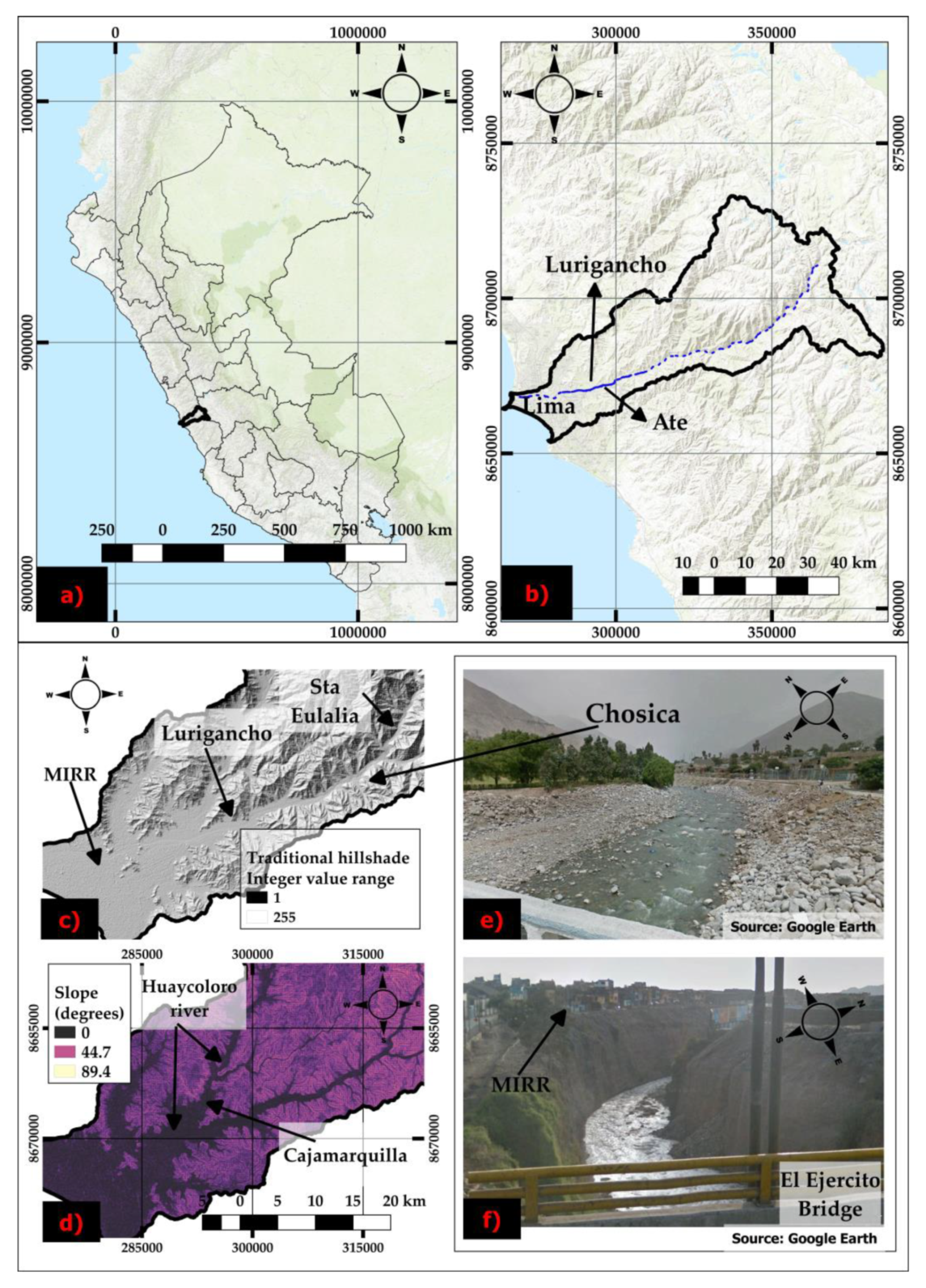
Figure 1. (a) Geographic location of the Rímac River basin in the central-western region of Peru and (b) its boundaries, with the blue line marking the river course. (c) Hillshade and (d) slope of the basin downstream of the confluence between the Alto Rímac and Santa Eulalia rivers, with indication of locations and toponyms of interest. Google Earth StreetView pictures showing: (e) the geomorphology of the open canyon at Chosica, as opposed to (f) the narrow urban canyon downstream at El Ejercito bridge, with nearly vertical cliffs above which the Margen Izquierda del Río Rímac (MIRR) shantytown was built along the left riverbank.
Applsci 10 06598 g001
Figure 2. Sentinel-2 images collected on (a) 28/12/2015 showing the typical cloud cover in Lima and on (b) 22/03/2017 during the catastrophic flooding event analyzed in this paper. Contains Copernicus Sentinel-2 data 2015, 2017.
Applsci 10 06598 g002
Figure 3. (a) Mean annual precipitation projected to 2030 (data source: [55]) and (b) precipitation anomaly in the period between December 2016 and February 2017 (data source: [60]).
Applsci 10 06598 g003
Figure 4. Flood events and El Niño phenomenon vs. availability of C-band synthetic aperture radar (SAR) satellite data from the European Remote-Sensing (ERS-1/2), ENVIronmental SATellite (ENVISAT) and Copernicus Sentinel-1 missions. The most intense events are indicated in blue.
Applsci 10 06598 g004
Figure 5. Example of change patterns in the radar backscatter: (a,b) decrease and (c,d) increase of the radar backscatter, in (a,c) RGB composites (R = master; G = slave; B = slave) and in (b,d) the corresponding signals in the ratio maps (slave/master).
Applsci 10 06598 g005
Figure 6. Geographic information system (GIS)-based analysis workflow: datasets showing spatial distribution of hazard factors and elements at risk (i.e., alluvial deposits, slope and land cover) are integrated with the SAR-based red, green and blue (RGB) composites to detect and interpret the observed change patterns of radar backscatter as “Flooding” (F) and “No-Flooding” (NF) changes. Satellite optical imagery from Google Earth is exploited for validation. The same approach applies to the ratio maps.
Applsci 10 06598 g006
Figure 7. Distribution of the areas of the Rímac River basin where change patterns in the radar backscatter that are likely related with flooding were observed and mapped. Where visible, dashed lines indicate sections of rivers where no change patterns have been found (e.g., the narrow urban canyon downstream displayed in Figure 1f).
Applsci 10 06598 g007
Figure 8. Example of F1 “Flooded areas” changes in relation to the 16/03/2017 flood event: (a) Sentinel-1 RGB composite and (b) ratio map. The blue rectangles indicate the path of the Rímac River, and the red rectangle the urban area affected by the flood event. Google Earth imagery (© 2020 Maxar Technologies) acquired (c) before (22/02/2017) and (d) after (21/03/2017) the event. Contains modified Copernicus Sentinel-1 data.
Applsci 10 06598 g008
Figure 9. Example of F2 “Riverbed flooded by increased water flow” changes occurred in relation to the 16/03/2017 flood event: (a) Sentinel-1 RGB composite and (b) ratio map highlight a clear change pattern of radar backscatter decrease (light green polygon) caused by the increase in the flow of the Rímac River. Google Earth images (© 2020 Maxar Technologies) show the condition of the riverbed in (c) the dry (16/12/2016) and (d) rainy (17/03/2017) season. Contains modified Copernicus Sentinel-1 data.
Applsci 10 06598 g009
Figure 10. Example of F3 “Riverbank collapses and damages” changes in relation to the 31/01/2017 flood event: (a) Sentinel-1 RGB composite and (b) ratio map highlight a pattern of decreased radar backscatter due to the increase in the water flow and level of the Rímac River (blue polygon) and local collapse of the riverbank (pink polygon). Google Earth imagery (© 2020 Maxar Technologies) acquired (c) before (28/01/2017) and (d) after (18/03/2017) the event, with (e) matching profile views evidencing the detachment niche due to the riverbank collapse. Contains modified Copernicus Sentinel-1 data.
Applsci 10 06598 g010
Figure 11. Google Earth imagery (© 2020 Maxar Technologies) acquired on (a) 28/01/2017 and (b) 21/03/2017 showing the Talavera Bridge prior and after the collapse due to the 16/03/2017 flood event, respectively. In (b) the increase of the water flow of the Rímac River is apparent.
Applsci 10 06598 g011
Figure 12. Google Earth synoptic view of the riverbank (red circle; see Figure 10e) and the Talavera Bridge (red square; see Figure 11) collapses on 26/03/2017.
Applsci 10 06598 g012
Figure 13. Distribution of changes in the radar backscatter, likely due to human activities (anthropogenic), observed and mapped within the Rímac River basin.
Applsci 10 06598 g013
Figure 14. Example of NF1 changes “Motorway construction”: (a) Sentinel-1 RGB composite and (b) ratio map show opposite patterns in the radar backscatter caused by (c,d) activities for road construction, as indicated in the 23/11/2016 and 28/01/2017 optical imagery (Google Earth images © 2020 Maxar Technologies). Contains modified Copernicus Sentinel-1 data.
Applsci 10 06598 g014
Figure 15. Example of NF2 change “Vegetation cover—cropland changes”: (a) ERS-2 RGB composite and (b) ratio map of the cross-event pair 10/04/1996—20/05/1998 (see Appendix A, Table A1) show a clear pattern of radar backscatter decrease in Las Praderas de Pariachi on the left bank of the Rímac River that, until mid-1996, was occupied by agricultural fields and, afterwards, was subject to urban sprawl, in specific for the development of the residential district [48]. The land-cover transition is confirmed in the band combination 7-4-2 (“natural-like” [89]) of Landsat 4-5 Thematic Mapper (TM) images collected on (c) 14/04/1996 and (d) 22/05/1998.
Applsci 10 06598 g015
Figure 16. Examples of NF3 change “Ephemeral changes” and NF9 change “New building constructions”. (a) ERS-2 RGB composite and (b) ratio map highlight patterns of increased radar backscatter, in one case matching with (c) vehicles parked near the principal wholesale fruit market in Lima, in the other with (d) the start of the construction activities of the Jockey Plaza shopping center (April 1996) [90].
Applsci 10 06598 g016
Figure 17. Example of NF13 change “Archaeological excavations”: (a) Sentinel-1 RGB composite and (b) ratio map highlight a decrease in radar backscatter (dark lilac polygon) in an archaeological site where fires may have altered the vegetation coverage, as identified in the optical imagery acquired on (c) 08/02/2017 and (d) 03/03/2017 (Google Earth images © 2020 Maxar Technologies). Contains modified Copernicus Sentinel-1 data.
Applsci 10 06598 g017
Figure 18. Map of flooding risk classification at basin scale over Lima, based on the combination of satellite SAR evidence and natural (Figure 7) and anthropogenic factors (Figure 13) of flooding hazard, vulnerability and exposed elements.
Applsci 10 06598 g018
Figure 19. Comparison between (a) the Sentinel-1 ratio map of the areas inundated during the March 2017 flooding event and (b) the potential maximum flood extent (cyan polygon) produced by Copernicus Emergency Management Service (EMS) during the Risk and Recovery Activation EMSN-038 [44].
Applsci 10 06598 g019
Figure 20. Comparison between (a) the flooding risk classification map generated in this research and (b) the map of flooding susceptibility and fluvial erosion published by Villacorta et al. [28], to highlight (c) the mutual spatial overlap and risk classification differences.
Applsci 10 06598 g020
Table 1. Extraordinary El Niño events and dates of major floods in the Rímac River basin.
Extraordinary EventsNumber of Flood EventsDates of Flooding in Urban Areas
1982–1983Data n.a.December 1982–June 1983
1997–1998609/02/1998
23/02/1998
2017–20181314/01/2017
31/01/2017
16/03/2017
14/02/2018
22/02/2018
Table 2. Key technical features of the SAR data used in this study. Notation: IM—Image Mode; IW—Interferometric Wide; SLC—Single Look Complex; GRD—Ground Range Detected; V—Vertical; H—Horizontal.
SatelliteLaunch and End of OperationsProduct LevelRevisit Time (Days)PolarizationModeBandSwath (km)Ground Range Resolution (m)
ERS-1/21991/1995
2000/2011
Level 1
SLC
35VVIMC10025
Sentinel-1B2016
-
Level 1
GRD
12VV+VHIWC2505 (single look)
Table 3. SAR image working pairs made of ERS-1/2 and Sentinel-1 scenes over Lima, Peru.
SAR Image Working PairsPre-EventCross-EventPost-EventTotal Number of SAR Working Pairs
1997–19981449
2017–201810101030
Table 4. Ancillary data over Lima (Peru) used in the geospatial analysis in the QGIS environment. Acronyms: ASTER - Advanced Spaceborne Thermal Emission and Reflection Radiometer; GDEM - Global DEM.
TypologyDescriptionFormatSpatial Resolution and/or ScaleReference DateSource
AnthropogenicAdministrative boundariesShapefile1:100,000-Geocatmin [72]
Census data (population/households)Shapefile1:100,0002011Geocatmin [73]
Urban land coverRaster12 m2011Global Urban Footprint [74,75]
Open Street MapRaster--QGIS desktop v.3.2.3 service
NaturalHydrographic basinShapefile1:175,000-Ministerio del Ambiente-MINAM [76]
ASTER GDEM v.2Raster1 arcsec
(30 m)
2011USGS-NASA [77]
Topographic contour linesShapefile1:100,000-GEO_GSP_PERU [78]
GeologyShapefile1:100,000-GEO_GSP_PERU [79]
Global Surface WaterWeb Map Service-1984–2019EC JRC/Google [80,81]
BasemapSentinel-2 image (cloud-free)Raster-2016Scihub
Google Earth basemapHtml (cache)--Google Earth
Table 5. Description of the categories of changes related to the studied flood events.
Category Code Flooding (F)DescriptionNumbers of ChangesArea (km2)
Flooded areas (F1)Areas that have been affected by the flood events in the years 1997–1998 and 2017–2018.1518.90
Riverbed flooded by increased water flow (F2)Areas of the riverbed of the Rímac River which, due to an increase in its flow rate, have been submerged totally or partially.17512.70
Riverbank collapses and damage (F3)Riverbed areas of the Rímac River (bordering the banks) which, as a consequence of the increase in its flow rate, have been totally or partially removed, causing damage to infrastructure or houses.70.50
Table 6. Description of the changes categories in the radar backscatter related to anthropogenic events. Numbers reported in parenthesis indicate how many changes of the total for the given category were considered for the subsequent flood risk assessment due to their local slope or proximity to the Rímac River. Grey background mark the categories of changes that were not relevant for flood risk zoning.
Category Code
No Flooding (NF)
DescriptionNumbers of ChangesArea
(km2)
Motorway construction
(NF1)
Construction of the highway called “Nuova Autopista Centrale (NAC)” (New Central Highway)373.30
Vegetation cover–cropland changes
(NF2)
Increase or decrease in vegetation cover (sowing/harvesting). Also included cultivated areas that have suffered a variation in land use27 (18)5.50
Ephemeral changes
(NF3)
Parked vehicles (e.g., trucks, goods loading/unloading activities). They are located near the sales companies or factories of different types of products150.60
NF4Machinery sales areas20.30
NF5Vehicle traffic452.90
NF6Raising water content in the treatment tanks. These changes have been identified in the water/waste treatment plants90.70
Landfill-earthworks
(NF7)
Soil deposit, to prepare the area for a change in land use7 (2)0.20
NF8Soil movement, identified as quarry zones221.80
New building constructions
(NF9)
New construction areas (sheds/new urban areas)26 (5)8.40
NF10Warehouse areas102.30
NF11Cemetery area10.01
Road construction
(NF12)
Roads under construction (Moralez duarez/Lurigancho/Gambetta)7 (1)0.18
Archaeological excavations
(NF13)
Archaeological remains40.20
Table 7. Characteristics of the observed change patterns in the radar backscatter.
Type of ChangeSlope (Class)Alluvial DepositsUrbanNon-Urban
F1B-D
F2A-B
F3A-B
NF1A
NF2A
NF3A-B
NF7B
NF9A
NF12A
NF13A