Author Contributions
Conceptualization, Ó.M.-C., M.D.-R., I.d.C. and V.M.; methodology, Ó.M.-C., M.D.-R., I.d.C. and V.M.; software, Ó.M.-C., M.D.-R., I.d.C. and V.M.; validation, Ó.M.-C., M.D.-R., I.d.C. and V.M.; investigation, Ó.M.-C., M.D.-R., I.d.C. and V.M.; writing—original draft preparation, Ó.M.-C. and I.d.C.; writing—review and editing, Ó.M.-C. and I.d.C. All authors have read and agreed to the published version of the manuscript.
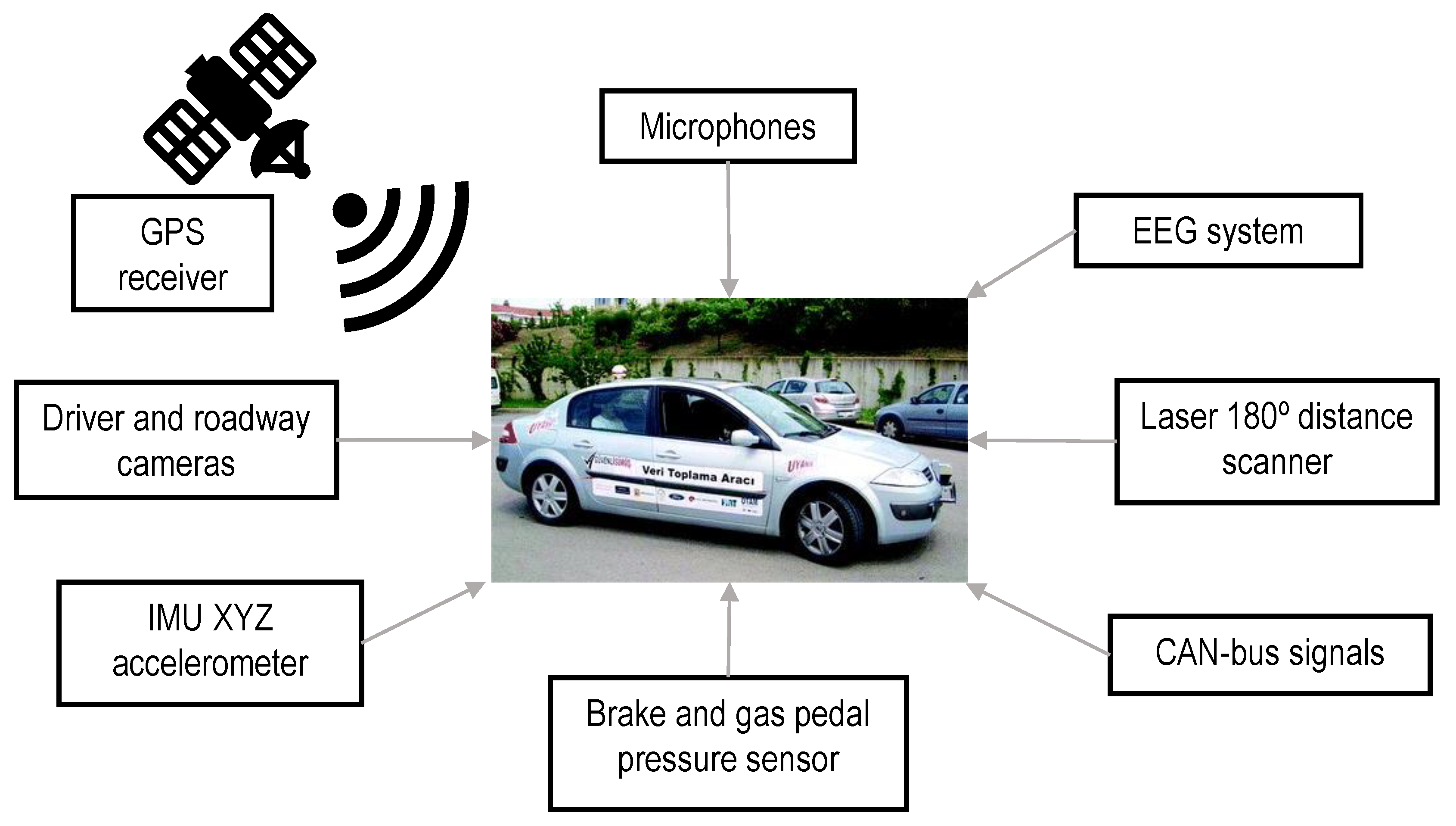
Figure 1.
Data-acquisition systems and sensors installed in the Uyanik car [
45].
Figure 1.
Data-acquisition systems and sensors installed in the Uyanik car [
45].
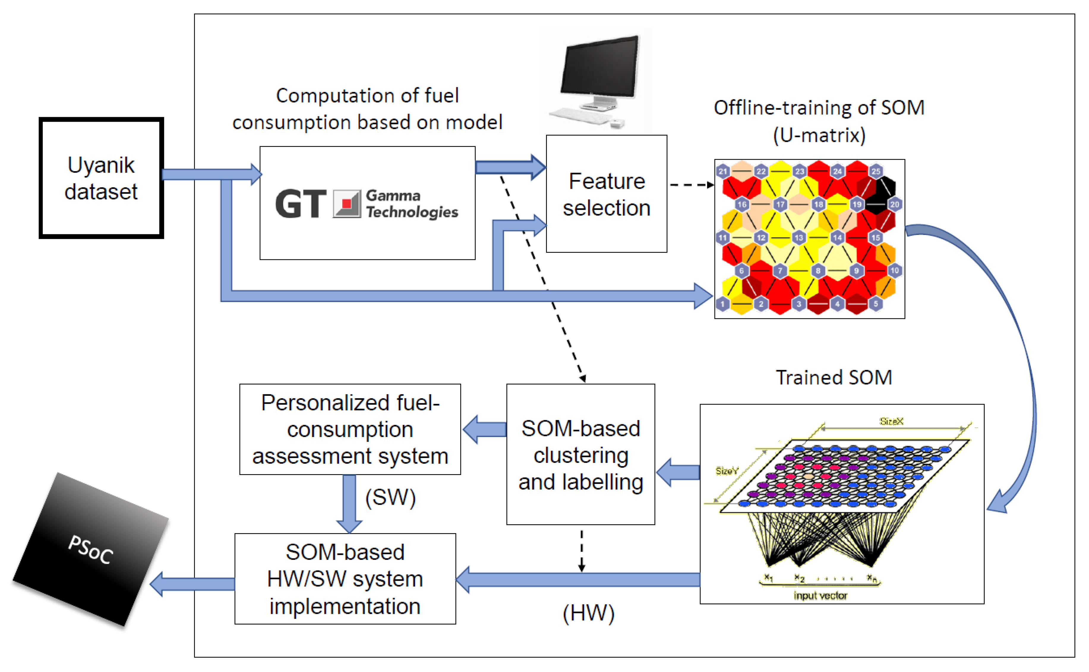
Figure 2.
Offline sequence of tasks involved in the design and development of an self-organized map (SOM)-based intelligent system for fuel consumption assessment. The dotted arrows indicate that the simulated fuel consumption data are also used to label the SOM-based clustering for verification purposes and to elaborate the hardware (HW) implementation of the SOM.
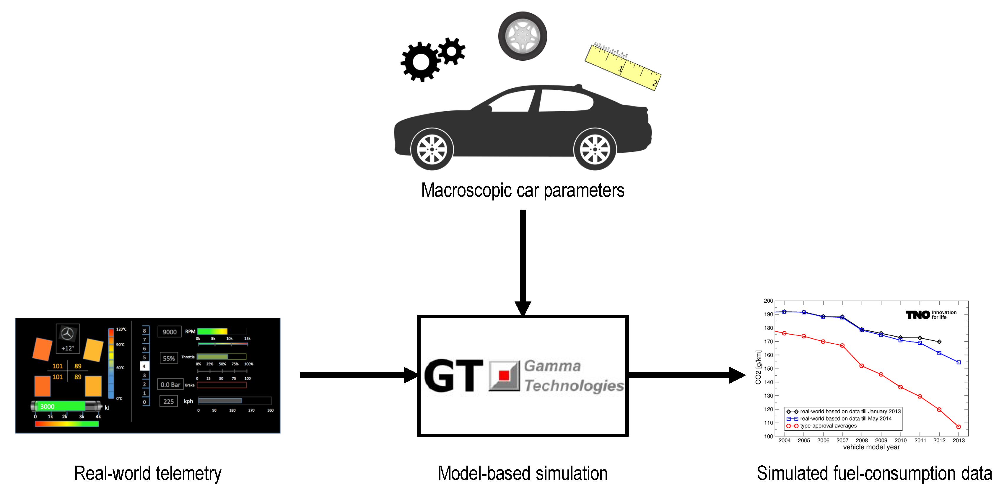
Figure 3.
Flow of real-world telemetry-based fuel consumption simulation. It has macroscopic car parameters (gear ratios, tyre dimensions, and wheelbase) and telemetry (gas pedal, brake pedal, speed, selected gear, and accelerations) as inputs. The model returns the simulated fuel flow as output.
Figure 3.
Flow of real-world telemetry-based fuel consumption simulation. It has macroscopic car parameters (gear ratios, tyre dimensions, and wheelbase) and telemetry (gas pedal, brake pedal, speed, selected gear, and accelerations) as inputs. The model returns the simulated fuel flow as output.
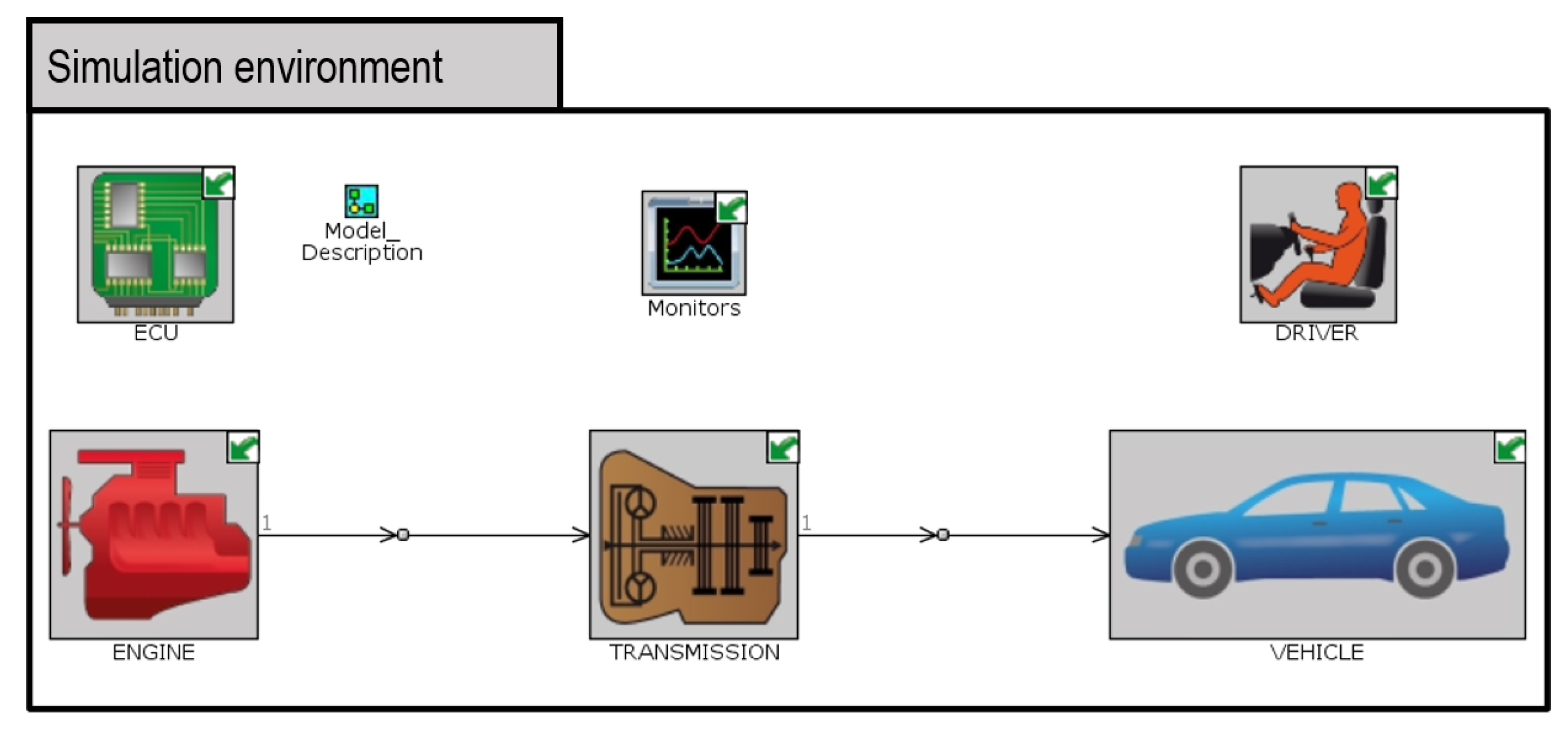
Figure 4.
Block diagram of real-world telemetry-based fuel consumption simulation of Uyanik Renault Mégane 1.5 dCi Sedan 74 kW. It has macroscopic car parameters (gear ratios, tyre dimensions, and wheelbase) and telemetry (gas pedal, brake pedal, speed, selected gear, and accelerations) as inputs. The model returns the simulated fuel flow as output.
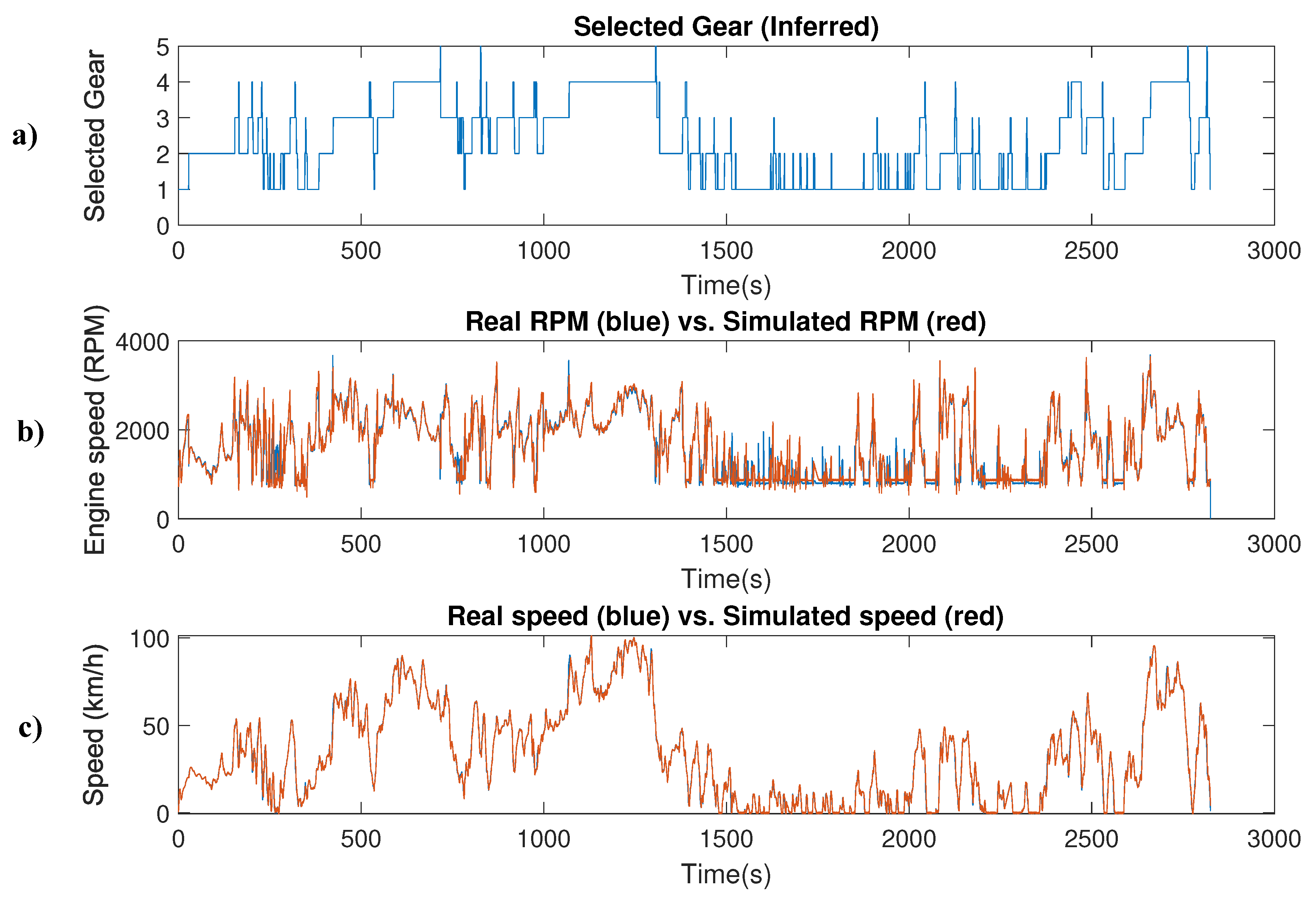
Figure 5.
Comparison of measured data vs. simulation results. (a) The inferred gear considering the computed rpm/speed ratios. (b) The measured revolutions per minute (RPM) of the vehicle vs. the RPM simulated by the model. (c) The measured speed of the vehicle vs. the speed simulated by the model.
Figure 5.
Comparison of measured data vs. simulation results. (a) The inferred gear considering the computed rpm/speed ratios. (b) The measured revolutions per minute (RPM) of the vehicle vs. the RPM simulated by the model. (c) The measured speed of the vehicle vs. the speed simulated by the model.
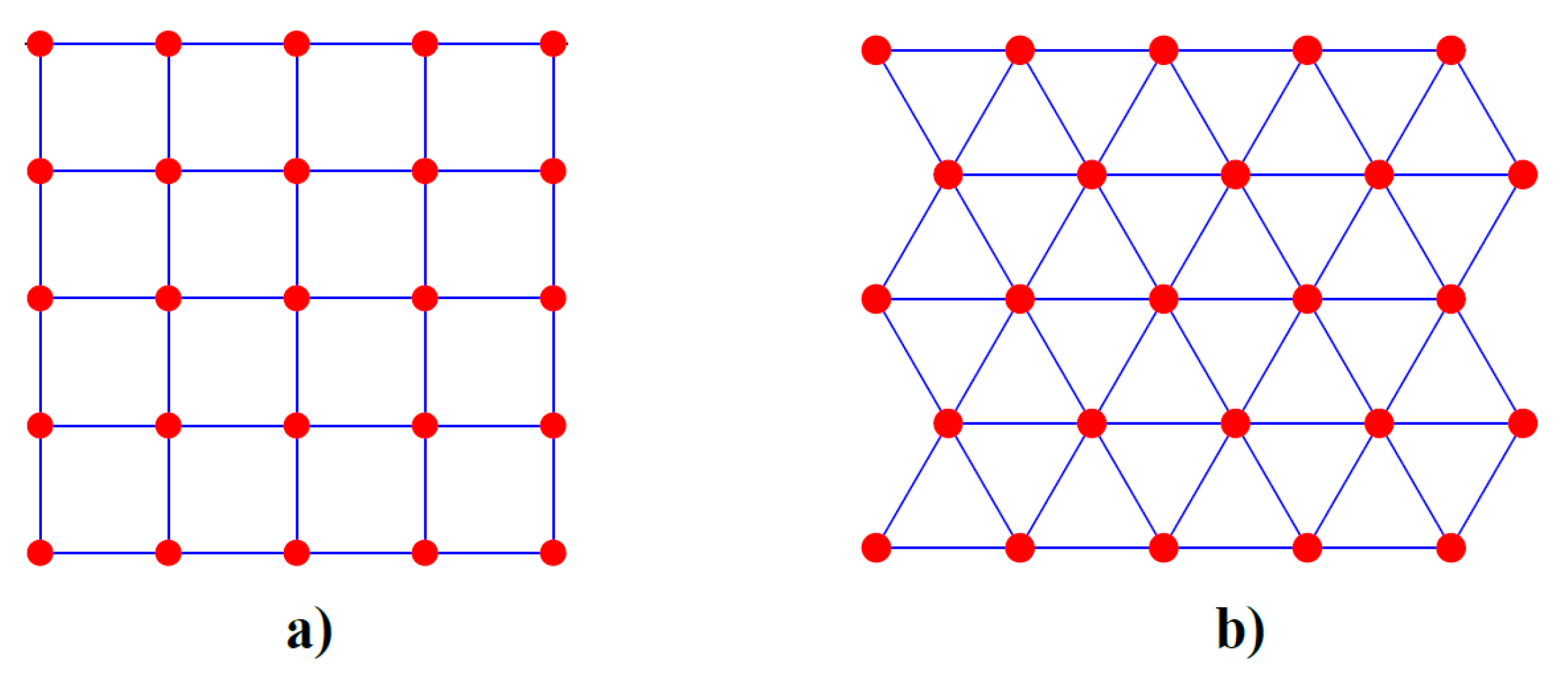
Figure 6.
Typical SOM topologies: a rectangular output grid (a) and a hexagonal output grid (b).
Figure 6.
Typical SOM topologies: a rectangular output grid (a) and a hexagonal output grid (b).
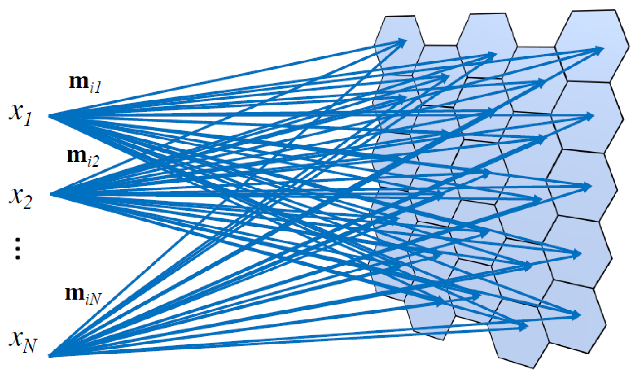
Figure 7.
Structure of an SOM with N inputs, , and M = 25 output neurons distributed into a 5 × 5 two-dimensional hexagonal grid.
Figure 7.
Structure of an SOM with N inputs, , and M = 25 output neurons distributed into a 5 × 5 two-dimensional hexagonal grid.
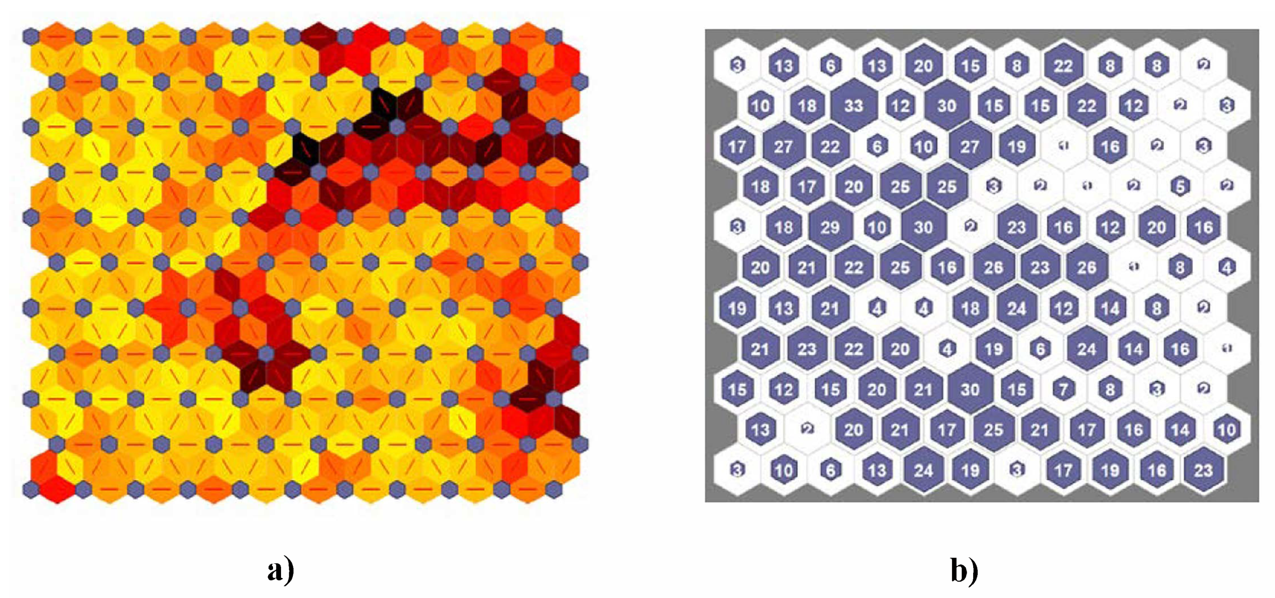
Figure 8.
SOM organized into an 11 × 11 neuron grid. (a) Neighbor weight distances. The blue hexagons represent the output neurons, while the red lines are neuron connections. Darker colors represent larger distances between neighboring neurons, and lighter colors represent smaller ones. (b) Sample hits. This image shows how many training samples are associated with each neuron.
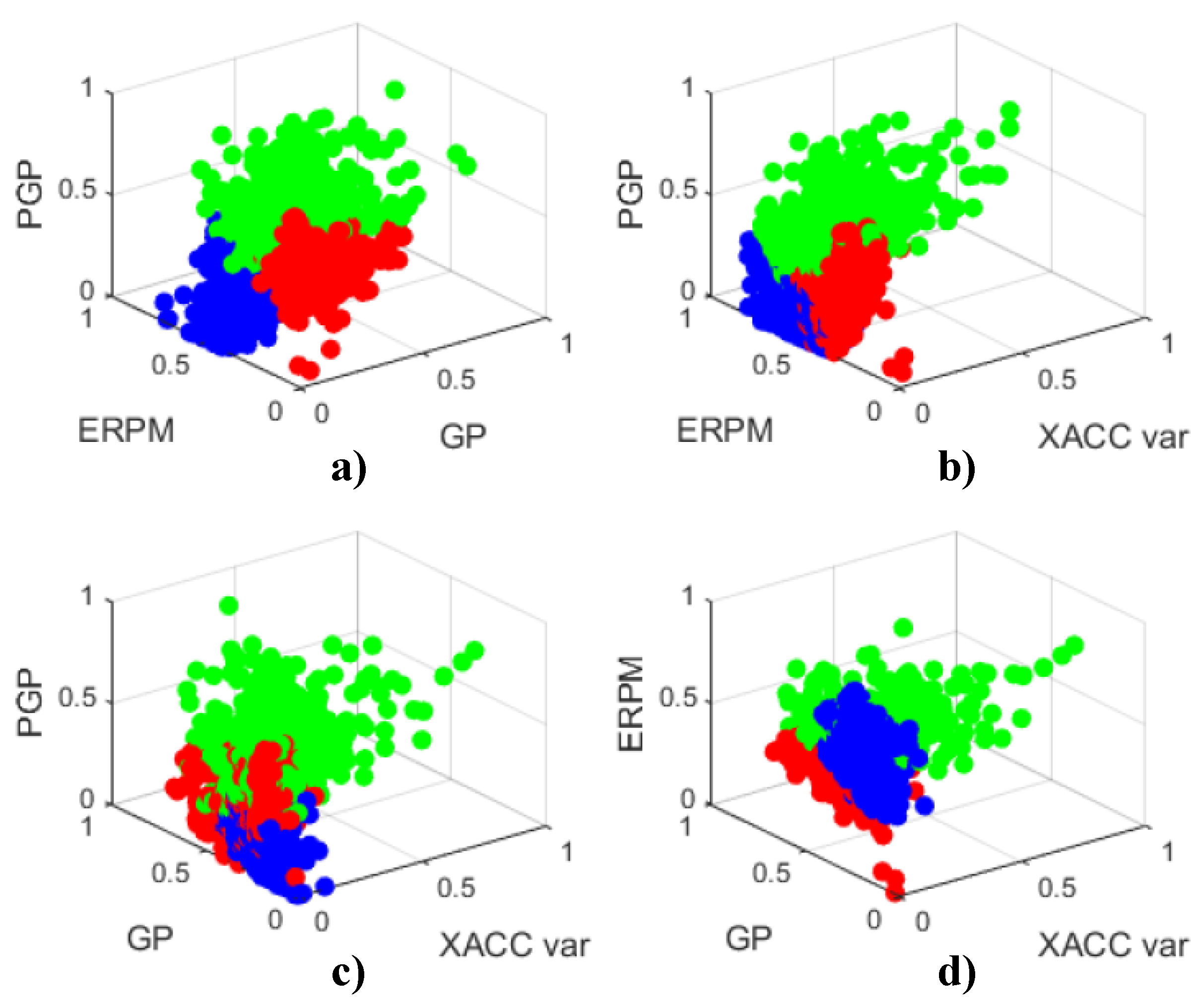
Figure 9.
Three-dimensional views of the three-cluster fuel consumption classification results. The clusters were labeled as Very low (red), Low (blue), and Medium-High (green). (a) Displays the cluster distribution considering PGP, ERPM and GP. (b) Considers PGP, ERPM and XACC var. (c) Displays clusters regarding PGP, GP and XACC var, and (d) considers ERPM, GP and XACC var.
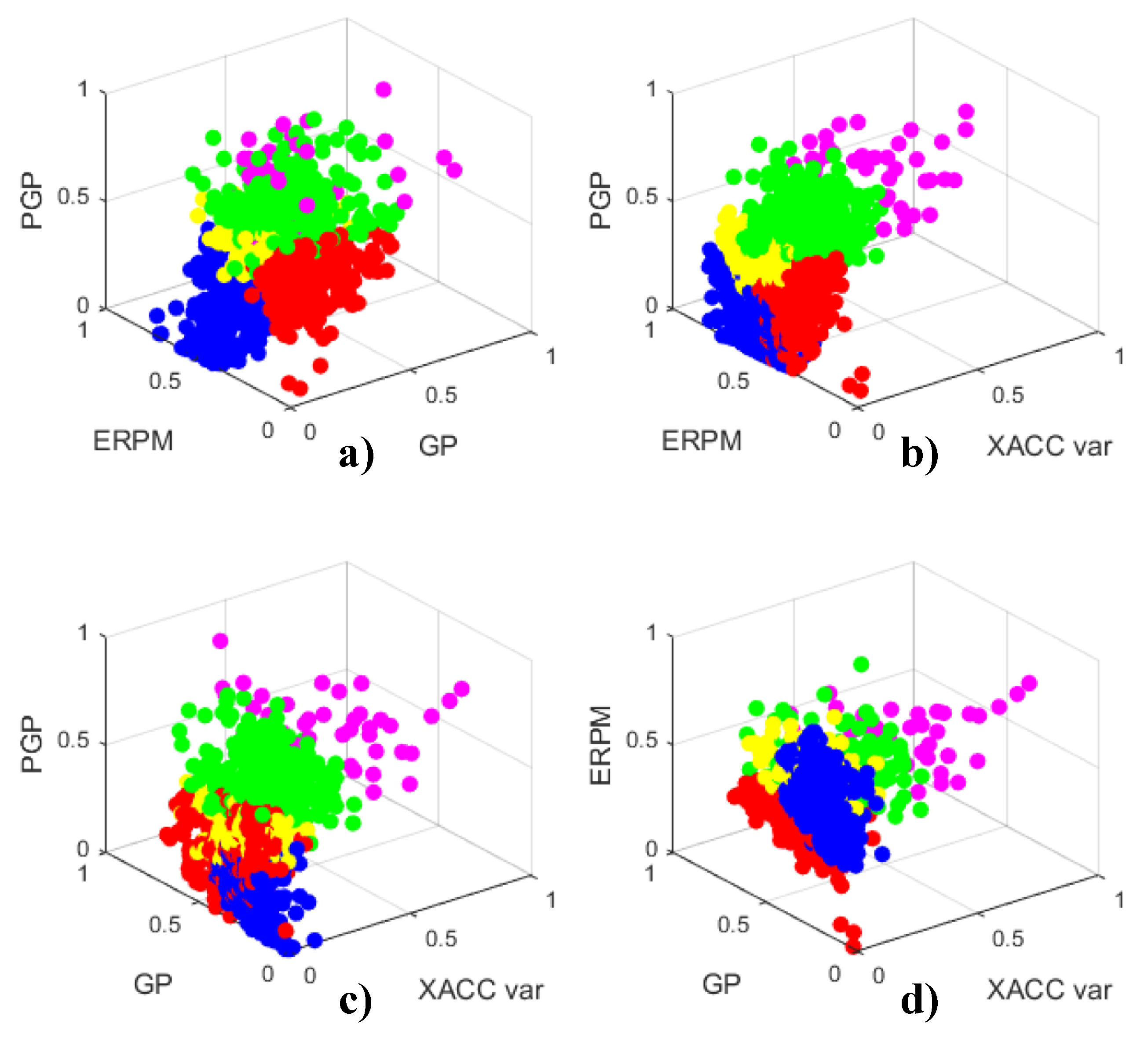
Figure 10.
Three-dimensional views of the five-cluster fuel consumption classification results. The clusters were labeled as Very low (red), Low (blue), Medium (yellow), High (green), and Very high (magenta). (a) Displays the cluster distribution considering PGP, ERPM and GP. (b) Considers PGP, ERPM and XACC var. (c) Displays clusters regarding PGP, GP and XACC var, and (d) considers ERPM, GP and XACC var.
Figure 11.
Uyanik measurement of relevant CAN-bus and IMU signals corresponding to D1 (green) and D11 (red) during five uninterrupted minutes of the route. The driving behavior was evaluated every 100 s, and the cluster with the maximum percentage was selected. Both D11 and D1 were classified into a single cluster during the whole segment of the trip: D11 drives according to the Very low cluster, and D1’s driving style is mostly into the Medium cluster. GT-Suite simulations of fuel consumption are also displayed.
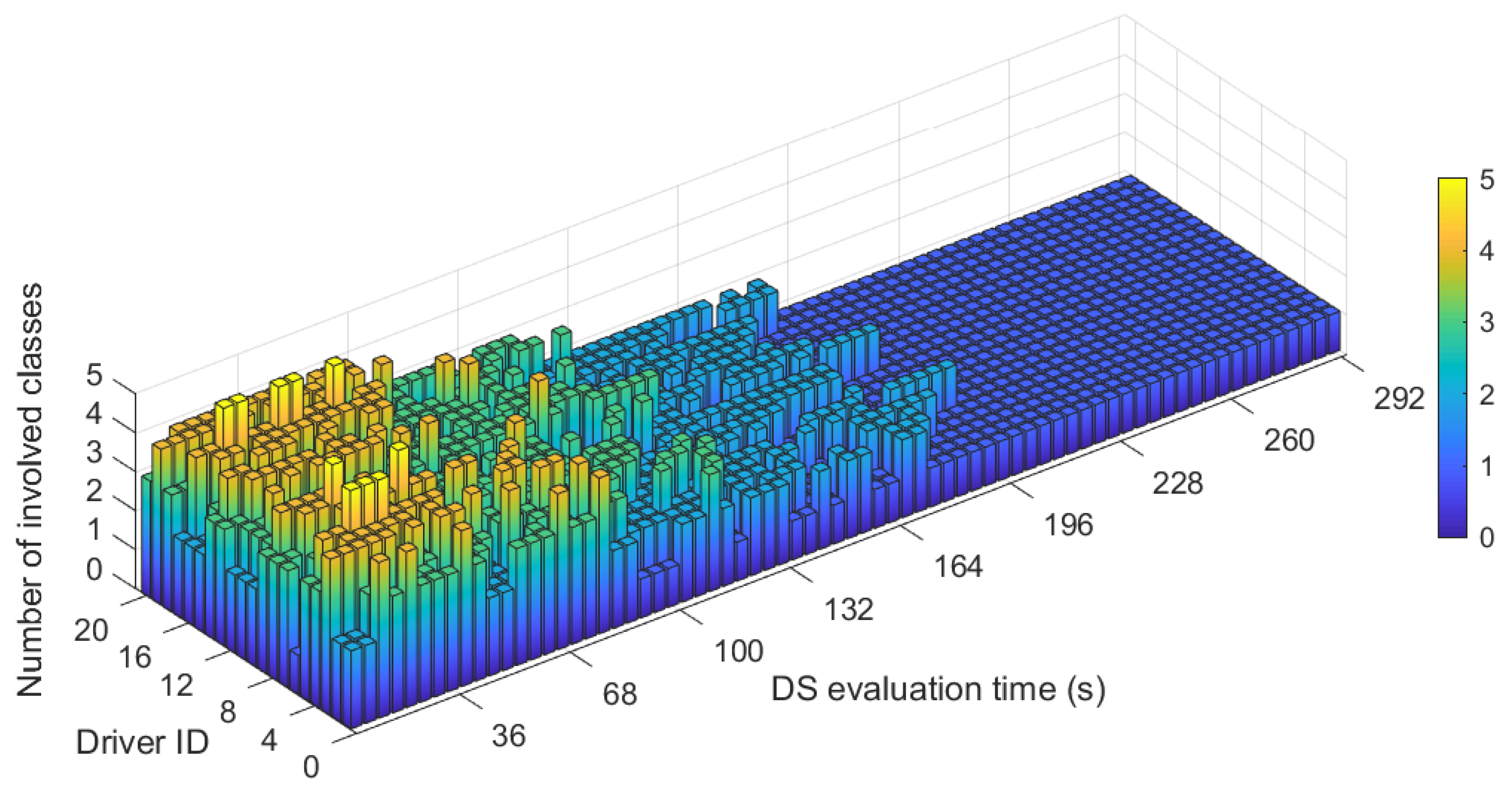
Figure 12.
Three-dimensional bar diagram of the number of classes identified, depending on the evaluation time for each driver.
Figure 12.
Three-dimensional bar diagram of the number of classes identified, depending on the evaluation time for each driver.
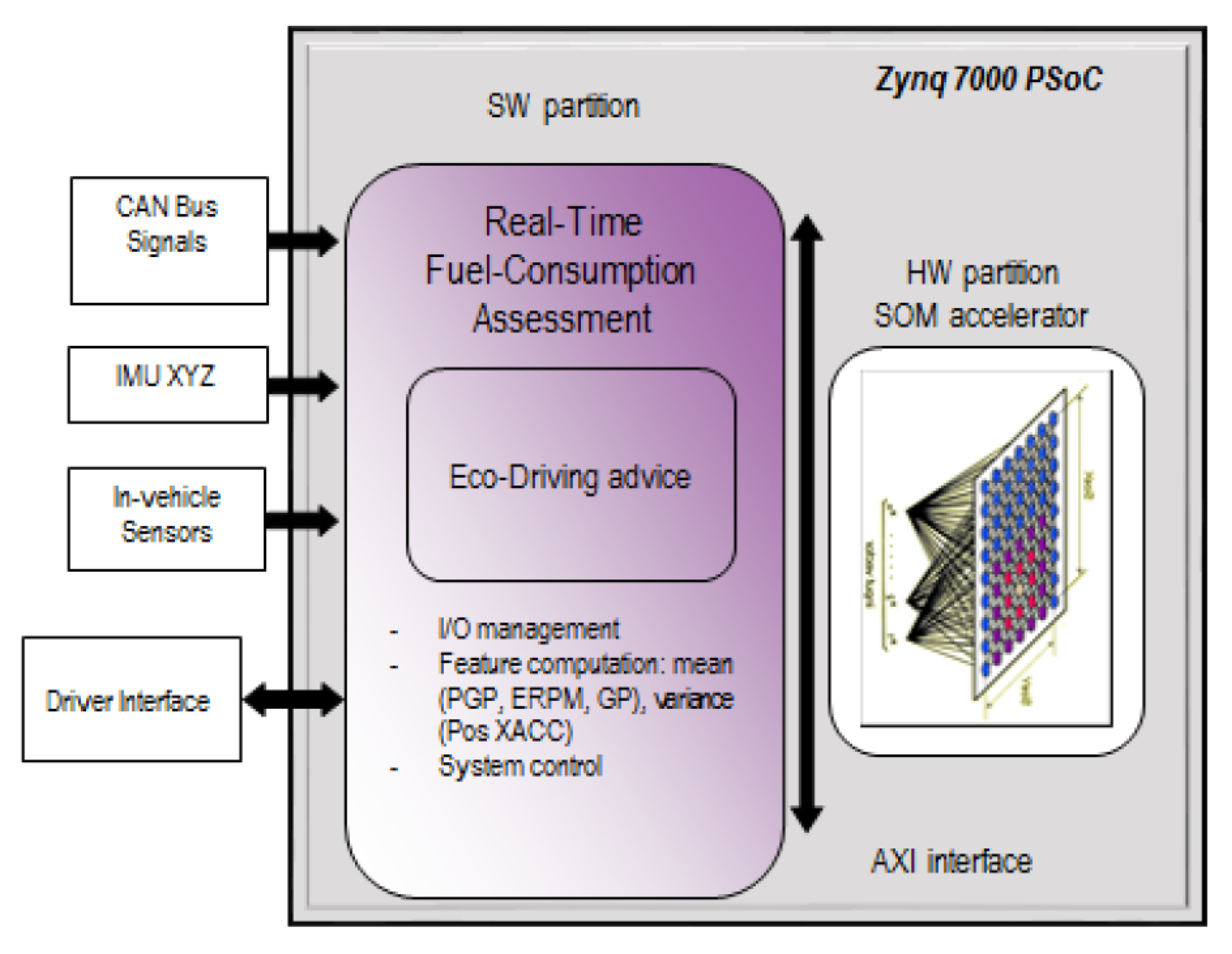
Figure 13.
Block diagram of the programmable system-on-a-chip (PSoC) for real-time fuel consumption assessment and eco-driving.
Figure 13.
Block diagram of the programmable system-on-a-chip (PSoC) for real-time fuel consumption assessment and eco-driving.
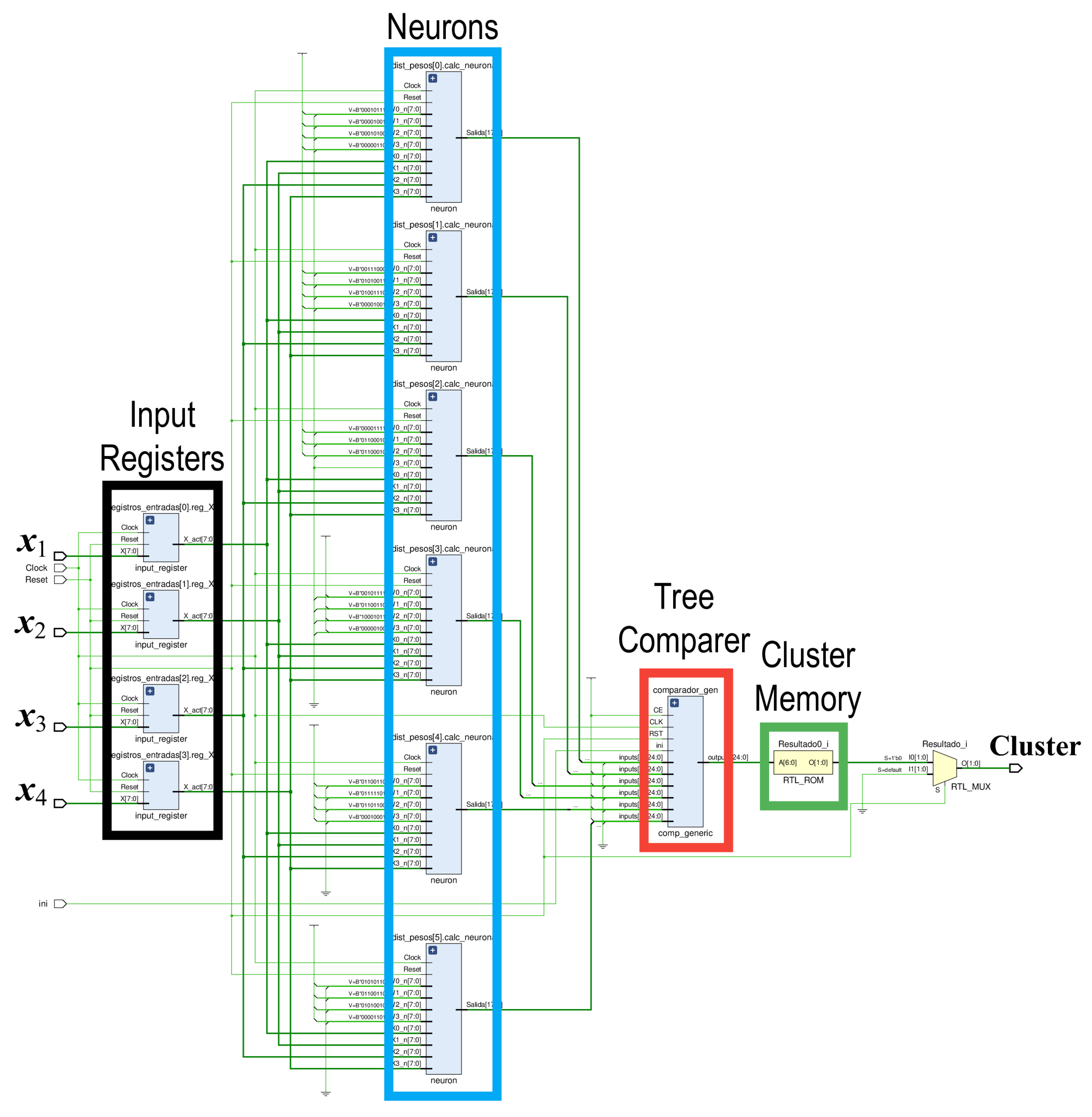
Figure 14.
Scheme of the SOM hardware accelerator. A four-input SOM topology with six output neurons is shown as a case example.
Figure 14.
Scheme of the SOM hardware accelerator. A four-input SOM topology with six output neurons is shown as a case example.
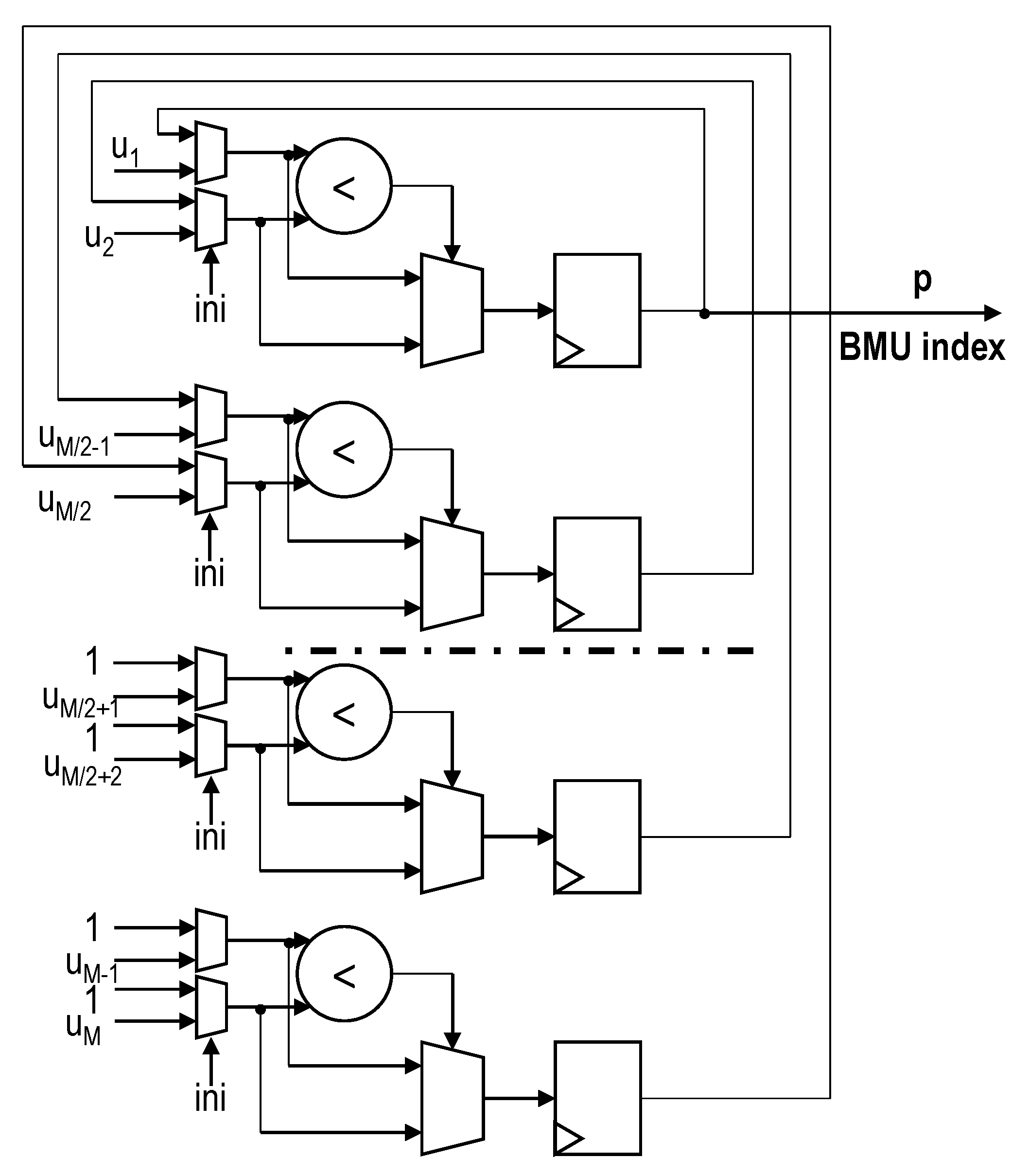
Figure 15.
Scheme of the proposed recursive tree comparer architecture that substitutes a traditional comparer solution.
Figure 15.
Scheme of the proposed recursive tree comparer architecture that substitutes a traditional comparer solution.
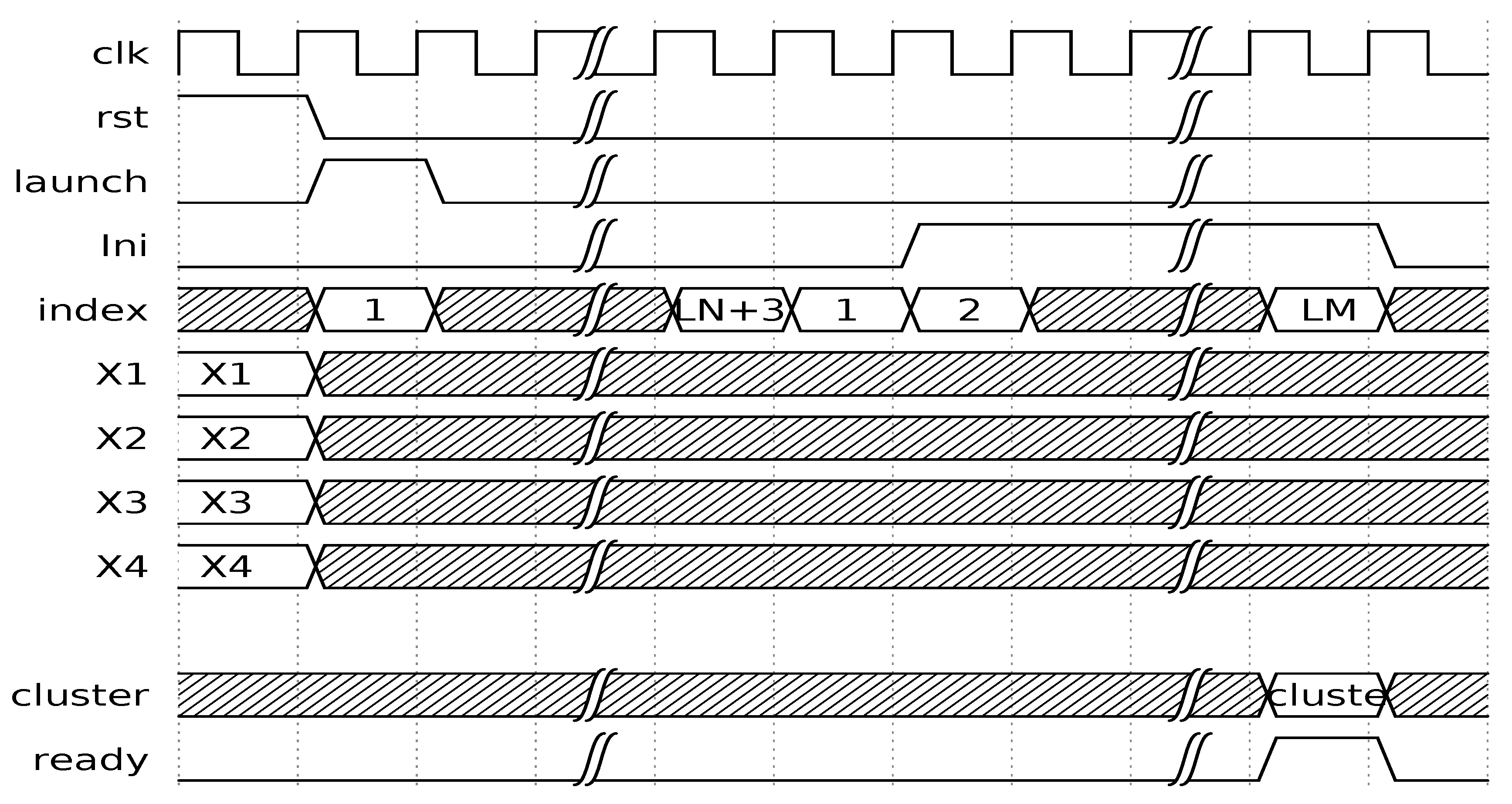
Figure 16.
Chronogram of the control-signal sequence of the SOM HW accelerator. LN stands for , and LM for .
Figure 16.
Chronogram of the control-signal sequence of the SOM HW accelerator. LN stands for , and LM for .
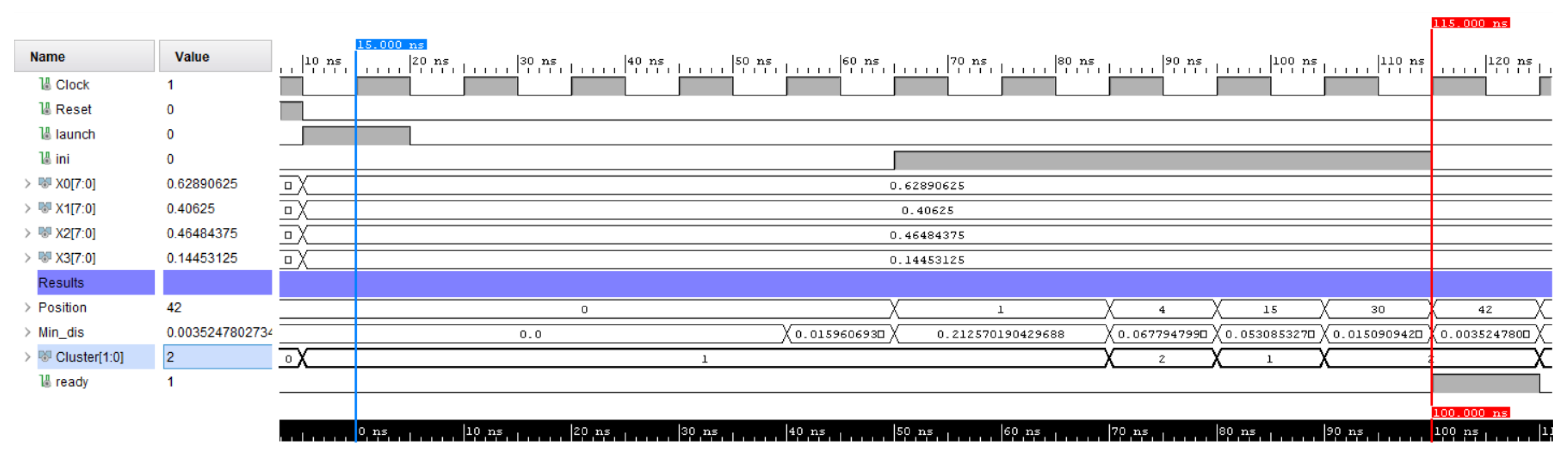
Figure 17.
Simulation results of the SOM HW accelerator obtained with the Vivado design suite.
Figure 17.
Simulation results of the SOM HW accelerator obtained with the Vivado design suite.
Table 1.
Significative variables of the Uyanik dataset [
45].
Table 1.
Significative variables of the Uyanik dataset [
45].
| Features | Signals (Time Series) |
|---|
| CAN bus | Steering wheel angle (SWA) |
| Steering wheel speed (SWS) |
| Vehicle speed (VS) |
| Percent gas pedal (PGP) |
| Engine RPM (ERPM) |
| Pressure sensors | Brake pedal pressure (BP) |
| Gas pedal pressure (GP) |
| IMU unit | Roll rate (RR) |
| Pitch rate (PR) |
| Yaw rate (YR) |
| X axis accelerometer (XACC) |
| Y axis accelerometer (YACC) |
| Z axis accelerometer (ZACC) |
| Laser | Distance to obstacle (d_90) |
| GPS | Coordinates (GPS) |
Table 2.
Driving behavior signals and Pearson correlation coefficients (PCCs) of fuel consumption with relevant features. Mean values and variances are computed using 8 s analysis windows.
Table 2.
Driving behavior signals and Pearson correlation coefficients (PCCs) of fuel consumption with relevant features. Mean values and variances are computed using 8 s analysis windows.
| Measurement Units | Signals (Time Series) | PCC: Mean | PCC: Variance |
|---|
| CAN-bus | Vehicle speed (VS) | 0.59 | 0.15 |
| Percent gas pedal (PGP) | 0.63 | 0.58 |
| Engine RPM (ERPM) | 0.66 | 0.18 |
| Pressure sensors | Brake pedal pressure (BP) | −0.35 | −0.23 |
| Gas pedal pressure (GP) | 0.52 | 0.20 |
| IMU unit | Positive X axis acceleration (Pos XACC) | 0.32 | 0.25 |
| Negative X axis acceleration (Neg XACC) | −0.17 | −0.11 |
Table 3.
Percentage of the route that each driver travels using different fuel-consumption driving styles (DSs) (three-cluster classification).
Table 3.
Percentage of the route that each driver travels using different fuel-consumption driving styles (DSs) (three-cluster classification).
| Driver | Very Low (%) | Low (%) | Medium-High (%) |
|---|
| D1 | 4.7 | 20.0 | 75.3 |
| D2 | 49.4 | 10.4 | 40.2 |
| D3 | 23.0 | 33.3 | 43.7 |
| D4 | 7.8 | 51.1 | 41.1 |
| D5 | 33.3 | 26.5 | 40.2 |
| D6 | 80.2 | 10.4 | 9.4 |
| D7 | 15.1 | 33.7 | 51.2 |
| D8 | 16.2 | 29.7 | 54.1 |
| D9 | 8.1 | 38.4 | 53.5 |
| D10 | 56.3 | 0 | 43.7 |
| D11 | 78.6 | 11.9 | 9.5 |
| D12 | 10.6 | 33.0 | 56.4 |
| D13 | 14.0 | 46.5 | 39.5 |
| D14 | 8.4 | 25.3 | 66.3 |
| D15 | 2.5 | 45.7 | 51.8 |
| D16 | 14.3 | 40.5 | 45.2 |
| D17 | 38.1 | 21.4 | 40.5 |
| D18 | 2.7 | 48.0 | 49.3 |
| D19 | 15.6 | 30.0 | 54.4 |
| D20 | 32.2 | 26.9 | 40.9 |
Table 4.
Fuel consumption (L/100km) parameters of the three-cluster classification.
Table 4.
Fuel consumption (L/100km) parameters of the three-cluster classification.
| Cluster Label | Average Value | Variance | Maximum Value |
|---|
| Very low (red) | 2.76 | 1.02 | 6.66 |
| Low (blue) | 3.04 | 1.53 | 7.80 |
| Medium-High (green) | 5.15 | 3.34 | 12.6 |
Table 5.
Actions that are associated to the three-cluster classification.
Table 5.
Actions that are associated to the three-cluster classification.
| Current Cluster | Required Action |
|---|
| Very low (red) | Keep driving style |
| Low (blue) | Lower RPM/Switch to a higher gear |
| Medium-High (green) | Lower RPM/Keep gas steady/Lower PGP |
Table 6.
Fuel consumption (L/100km) parameters of the five-cluster classification.
Table 6.
Fuel consumption (L/100km) parameters of the five-cluster classification.
| Cluster Label | Average Value | Variance | Maximum Value |
|---|
| Very low (red) | 2.75 | 1.04 | 6.66 |
| Low (blue) | 3.04 | 1.54 | 7.80 |
| Medium (yellow) | 4.44 | 2.21 | 10.1 |
| High (green) | 5.42 | 3.13 | 11.4 |
| Very high (magenta) | 7.81 | 5.38 | 12.5 |
Table 7.
Percentage of the route that each driver travels using different fuel-consumption DS (five-cluster classification).
Table 7.
Percentage of the route that each driver travels using different fuel-consumption DS (five-cluster classification).
| Driver | Very Low (%) | Low (%) | Medium (%) | High (%) | Very High (%) |
|---|
| D1 | 4.7 | 20.0 | 44.7 | 30.6 | 0 |
| D2 | 48.3 | 10.3 | 2.3 | 32.2 | 6.9 |
| D3 | 21.8 | 33.3 | 13.8 | 30.0 | 1.1 |
| D4 | 7.8 | 51.1 | 22.2 | 18.9 | 0 |
| D5 | 33.3 | 26.5 | 10.3 | 25.3 | 4.6 |
| D6 | 71.9 | 10.4 | 9.4 | 8.3 | 0 |
| D7 | 14.0 | 33.7 | 18.6 | 29.1 | 4.6 |
| D8 | 14.9 | 29.7 | 8.1 | 37.8 | 9.5 |
| D9 | 8.1 | 38.4 | 31.4 | 22.1 | 0 |
| D10 | 56.3 | 0 | 16.1 | 25.3 | 2.3 |
| D11 | 78.6 | 11.9 | 1.2 | 8.3 | 0 |
| D12 | 10.6 | 33.0 | 37.2 | 19.2 | 0 |
| D13 | 14.0 | 46.5 | 15.1 | 24.4 | 0 |
| D14 | 8.4 | 25.3 | 31.3 | 35.0 | 0 |
| D15 | 2.5 | 45.7 | 24.7 | 23.4 | 3.7 |
| D16 | 13.1 | 40.5 | 30.9 | 15.5 | 0 |
| D17 | 38.1 | 21.4 | 10.7 | 21.5 | 8.3 |
| D18 | 2.7 | 48.0 | 19.2 | 26.0 | 4.1 |
| D19 | 15.6 | 30.00 | 21.1 | 32.2 | 1.1 |
| D20 | 32.2 | 26.9 | 22.6 | 18.3 | 0 |
Table 8.
Actions associated to the five-cluster classification.
Table 8.
Actions associated to the five-cluster classification.
| Current Cluster | Required Action |
|---|
| Very low (red) | Keep driving style |
| Low (blue) | Lower RPM/Switch to a higher gear |
| Medium (yellow) | Lower RPM/Operate gas softly |
| High (green) | Lower PGP/Lower RPM |
| Very high (magenta) | Lower PGP/Keep gas steady |
Table 9.
Expected fuel-consumption reduction between contiguous clusters.
Table 9.
Expected fuel-consumption reduction between contiguous clusters.
| Current Cluster | Target Cluster | Reduction (%) |
|---|
| Low | Very low | 9.5 |
| Medium | Low | 31.5 |
| High | Medium | 18.1 |
Table 10.
Post-implementation resources report (Xilinx XC7Z045-2FFG900).
Table 10.
Post-implementation resources report (Xilinx XC7Z045-2FFG900).
| Resource | Utilization | Available | % Used |
|---|
| LUT | 21 107 | 218 600 | 9.66 |
| Flip-flops | 13 337 | 437 200 | 3.05 |


