An Intelligent and Cost-Efficient Resource Consolidation Algorithm in Nanoscale Computing Environments

Featured Application

Resource management in cloud computing environments.

Abstract

Because the Internet of things (IoT) and fog computing are prevalent, an efficient resource consolidation scheme in nanoscale computing environments is urgently needed. In nanoscale environments, a great many small devices collaborate to achieve a predefined goal. The representative case would be the edge cloud, where small computing servers are deployed close to the cloud users to enhance the responsiveness and reduce turnaround time. In this paper, we propose an intelligent and cost-efficient resource consolidation algorithm in nanoscale computing environments. The proposed algorithm is designed to predict nanoscale devices’ scheduling decisions and perform the resource consolidation that reconfigures cloud resources dynamically when needed without interrupting and disconnecting the cloud user. Because of the large number of nanoscale devices in the system, we developed an efficient resource consolidation algorithm in terms of complexity and employed the hidden Markov model to predict the devices’ scheduling decision. The performance evaluation shows that our resource consolidation algorithm is effective for predicting the devices’ scheduling decisions and efficiency in terms of overhead cost and complexity.

1. Introduction

The usage of the Internet and its applications has changed the world to the Internet of Everything (IoE). An extension of the Internet of things (IoT), the Internet of Nanothings (IoNT) has emerged as a new paradigm to incorporate the Internet into various domains, such as businesses, social networks, healthcare, teaching and learning techniques, and our daily activities [1,2,3]. RnR Market Research expects the IoT market to be worth about $1423.09 billion by 2020, and the IoNT will play a vital role in the future IoT market holdings by about $9.69 billion market value by 2020 [4].

Nanoscale devices (also called nanomachines or nanothings) can be connected with a nano-network to communicate and share appropriate data with each other, and these nanodevices in IoNT environments are able to monitor and detect tiny environmental changes and activities [5,6]. Body area networks, wireless sensor networks, and edge cloud networks can benefit from IoNT technology [7,8]. For example, regarding the edge cloud, mobile services using this can reduce latency and turnaround time [9,10].

Figure 1 shows an example of mobile services using IoNT with and without the edge cloud layer. Without this layer, when a user submits a task for the service, the sensing data from the nanodevices are forwarded to the central cloud server. Then, the central cloud server responds to the mobile device or application. However, in this scenario, the latency between the nanodevices and the central cloud server and the central cloud server and the mobile device is relatively long.

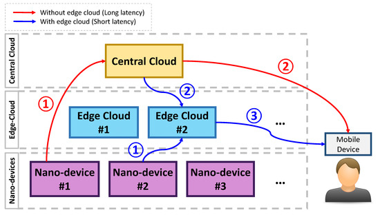
Figure 1. An example of mobile services using Internet of Nanothings (IoNT) with and without the edge cloud layer.

When the edge cloud is enabled in the architecture, the sensing data from the nanodevices are delivered to the nearby edge cloud server. This edge cloud server interacts with the central cloud server if needed and sends results back to the mobile device. Compared to the flow without the edge cloud layer, the latency is relatively short here. Although the latency is relatively short in this case, it is still necessary to determine whether to use the layer or not. To efficiently use the layer, we consider the cost of using the edge cloud server. That is, the central cloud server must send the appropriate data and offload the task to the edge cloud server for the service.

In this paper, we develop an intelligent and cost-efficient resource consolidation algorithm in nanoscale computing environments. The core concept of the proposed algorithm is to determine whether we should use the edge cloud layer by employing one of the artificial intelligence techniques (the hidden Markov model). The proposed resource consolidation algorithm considers the cost of using the edge cloud layer and effectively predicts the future application usage pattern, which is a difficult problem in cloud computing environments [11]. Then, it performs the task migration between the central cloud server and the edge cloud server for the service when necessary, which achieves the load balancing, one of the important features in cloud computing environments [12].

2. Background and Related Work

In this study, we employ the hidden Markov model [13], which determines whether we use the edge cloud layer or not. Given the hidden Markov model λ = (A, B, π) and a sequence of observations O = (O₀, O₁, …, O_T−1), our resource consolidation algorithm determines P(O | λ), where A is the state transition probabilities, B is an observation probability matrix, and π is the initial state distribution. Next, we uncover the hidden part of the hidden Markov model by finding an optimal state sequence for the underlying Markov process. Then, we determine a model of the form λ = (A, B, π) that maximizes the probability of O. For the details of the hidden Markov model, refer to [14,15].

Figure 2 depicts the hidden Markov model composed of hidden states and observed processes. We consider the observed process as monitoring information of the system and then calculate probabilities for the hidden states. Table 1 shows notations in the hidden Markov model.

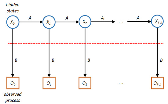
Figure 2. The hidden Markov model.

Table 1. Notations in the hidden Markov model (HMM).

Notation	Meaning
T	The length of the observation sequence.
N	The number of states in the model.
M	The number of observation symbols.
Q	The distinct states of the Markov process, that is, {q0, q1, …, qN−1}.
V	The set of possible observations, that is, {0, 1, …, M−1}.
A	The state transition probabilities.
B	The observation probability matrix.
π	The initial state distribution.
O	The observation sequence, that is, {O0, O1, …, OT−1}.
X	The hidden state sequence, that is, {X0, X1, …, XT−1}.

To calculate P(O|λ), we can determine the P(O|X,λ) by the definition of B as follows:

P(O|X,λ) = b_x0(O₀)b_x1(O₁) … b_xT−1(O_T−1),

(1)

where X is state sequences, that is, (x₀, x₁, …, x_T−1).

Then, it calculates P(X|λ) by the definitions of π and A as follows:

P(X|λ) = π_x0a_x0,x1a_x1,x2 … a_{xT−2,xT−1}.

(2)

Since P(O,X|λ) = P(O|X,λ)P(X|λ), we can determine P(O|λ) with state sequences as follow:

$$P(O|\lambda )={\sum }_X^{}P\left(O,X|\lambda \right)={\sum }_X^{}P(O|X,\lambda )P(X|\lambda ).$$

(3)

Next, to calculate the optimal state sequence, we define β_t(i) as follows:

β_t(i) = P(O_t+1, O_t+2, … O_T−1 | x_t = q_i, λ).

(4)

In addition, we define γ_t(i) for t = (0, 1, …, T−1) and i = (0, 1, …, N−1) as follows:

γ_t(i) = P(x_t = q_i|O,λ).

(5)

Since α_t(i) is for until t and β_t(_i) is after t, γt(i) can be calculated as follows:

γ_t(i) = α_t(i)β_t(i)/P(O|λ).

(6)

Thus, the optimal state at t is x_t = max γ_t(i). To illustrate the hidden Markov model, we use the parameters in Table 2. The parameter A = $\left[\begin{array}{cc}0.6& 0.4\\ 0.4& 0.6\end{array}\right]$ means that when the current state is stable (S), the probabilities that the next states will be stable (S) and unstable (U) are 60% and 40%, respectively, and when the current state is unstable (U), the probabilities that the next states will be stable (S) and unstable (U) are 40% and 60%, respectively. The parameter B = $\left[\begin{array}{ccc}0.1& 0.3& 0.6\\ 0.6& 0.3& 0.1\end{array}\right]$ means that when the current state is stable (S), the probabilities of the device’s state will be low (L), medium (M), and high (H) are 10%, 30%, and 60%, respectively, and when the current state is unstable (U), the probabilities that the device’s state will be low (L), medium (M), and high (H) are 60%, 30%, and 10%, respectively.

Table 2. Parameters for the illustrative example.

Parameter	Value
A	$\begin{array}{cc}& S|U\\ \hfill \frac{S}{U}& \left[\begin{array}{cc}0.6& 0.4\\ 0.4& 0.6\end{array}\right]\end{array}$
B	$\begin{array}{cc}& L\left|M\right|H\\ \hfill \frac{S}{U}& \left[\begin{array}{cc}0.1& \begin{array}{cc}0.3& 0.6\end{array}\\ 0.6& \begin{array}{cc}0.3& 0.1\end{array}\end{array}\right]\end{array}$
π	[0.4 0.6]
O	(2, 1, 0, 1, 1, 2, 1, 0)

The parameter π can be used when devices’ log information is unavailable, that is, the probabilities that the device is stable (S) and unstable (U) in the initial state are 40% and 60%, respectively. For the parameter O, we consider 0 as low (L), 1 as medium (M), and 2 as high (H). In this illustrative example, we do not consider the state transition from low (L) to high (H) or high (H) to low (L). Table 3 shows the calculated hidden Markov model probabilities for the sequence of SSUUSSUU. As the state sequence proceeds, the hidden Markov model probabilities change, which can be used to predict the device’s state for resource consolidation.

Table 3. HMM probabilities (the sequence is SSUUSSUU).

Sequence Number	Probability of S	Probability of U
0	0.8947576066	0.1052423934
1	0.5090529425	0.4909470575
2	0.1523176942	0.8476823058
3	0.4439562979	0.5560437021
4	0.5562550549	0.4437449451
5	0.8485699873	0.1514300127
6	0.4997196054	0.5002803946
7	0.1499719605	0.8500280395

Performance-aware resource management in cloud computing environments is challenging since it is hard to predict the system’s behavior [16], and it is also vital to reduce energy consumption for green cloud computing [17]. In [18], the authors proposed a cloud task mapping strategy for heterogeneity and hybrid architectures by considering various system metrics including response time, performance, and energy cost based on evolutionary games on a network equation for the task mapping. In [19], the authors proposed a two-phase queueing mechanism for scheduling cloud tasks by prioritizing the tasks based on constraints and service level agreements. It divides the cloud scheduling strategy into task assignment (by the central cloud server) and task scheduling (by each server in the cloud) phases.

To enable the Internet of things for the sensor-based big data analytics environment, the authors of [20] proposed a framework incorporating multiple core techniques (data collection, repository, data processing, analytics algorithms, wireless network, and data visualization) for smart and sustainable cities. To expand resource optimization techniques in the mobile edge cloud system, the authors of [21] proposed a partition technique for the mobile edge cloud clusters based on a graph-based algorithm to consolidate the network traffic in the mobile edge servers.

There are a few studies that incorporate an artificial intelligence technique for managing the mobile edge cloud resources. In [22], a deep reinforcement learning mechanism is used to overcome the high deployment and maintenance costs. With the learning technique, it adaptively allocates resources (computing and network) and reduces service time in mobile edge cloud environments. In [23], the authors used the hidden Markov model to detect multi-stage network attacks [24,25].

Although it used the same technique as ours, the scope and main objectives are different. The authors of [23] used the hidden Markov model to detect the network attack, but we use it to consolidate cloud resources in the mobile edge cloud environments. In addition, the above-mentioned studies did not incorporate predicting mobile devices’ stability information to resource management or scheduling algorithms.

3. The Proposed Resource Consolidation Algorithm

In this section, we detail the proposed resource consolidation algorithm for nanoscale computing environments. The proposed algorithm is based on the hidden Markov model to predict devices’ stability. In other words, when the edge server and the user’s device is stable, it determines to use the edge server, while when the edge server or the user’s device is unstable, it determines to use the cloud server without edge servers in the system.

Algorithm 1 shows the proposed resource consolidation algorithm. The input of the algorithm is the edge server list, the types of services for users’ requests, and users’ requests. After performing the resource consolidation algorithm, users’ requests are allocated to the edge servers or the central cloud server according to the specification of the algorithm. For the initialization, two Boolean variables (isAllocated and allocateEdge) are set to false.

Then, all the edge servers are also initialized by having no users’ requests. Of the two functions (checkRequests() and allocateRequests()), the checkRequests() function is performed first. Inside the function, all the users’ requests are checked and counted for the service types and frequency (lines 9–12). This procedure is necessary for the allocateRequests() function to allocate requests. Then, the requests are forwarded to the hidden Markov model process (line 11).

In the allocateRequests() function, the algorithm traverses each element of the users’ requests, then performs the treatment of less frequent requests, i.e., the frequency of the service type is counted as one (lines 15–17). For the less frequent services, the proposed resource consolidation algorithm allocates to the central cloud server. This is because, when it is allocated to the edge server, the algorithm introduces additional overheads by downloading appropriate data from the central cloud server. For the frequent services, it first checks the edge servers that are holding the same type of services (lines 19–25). In other words, when an edge server (ES_A) is running a healthcare service and the upcoming request’s service type is also the healthcare service, our resource consolidation algorithm allocates the upcoming request to ES_A so that no additional overheads are introduced.

Next, the countrequest variable for the edge servers is incremented by 1, and the isAllocated variable is set to true; these two variables are used when the algorithm cannot find the edge server holding the same type of service. If the isAllocated variable is false after performing the procedure of lines 19–25 (it cannot find the edge server holding the same type of service), the checkHMM() function is called (lines 26–27). The checkHMM() function returns true if its hidden Markov model’s maximum probability of O is to allocate the edge servers. Otherwise, the function returns false (the maximum probability of O is to allocate the central cloud server).

When the allocateEdge variable is true, then it allocates the request to the edge server whose count_request is lowest (lines 28–29). Note that this statement is useful since our resource consolidation algorithm can achieve the load balancing by allocating the request to the low-loaded edge server. Then, its count_request is incremented by one. Otherwise, (allocateEdge is false); it allocates the request to the central cloud server.

Algorithm 1 The proposed resource consolidation algorithm

Input:edgeServers [i], ∀i ∈ {1 … maxedge};

Services [j], ∀j ∈ {1 … maxservice};

Requests [k], ∀k ∈ {1 … maxrequest};

1: Output: Allocation of requests to edge servers or the central cloud server

2: Initialization: isAllocated ← false, allocateEdge ← false;

3: for all edgeServers[i] do

4:    edgeServer[i] ← null;

5: end for

6: call checkRequests();

7: call allocateRequests();

8: function checkRequest()

9:     for all requests[k] do

10:         requests[k].services[j].freq += 1;

11:         put requests[k] to HMM process;

12:    end for

13: end function

14: function allocateRequests()

15:    for all requests[k] do

16:        if requests[k].services[j].freq == 1 then

17:            allocate requests[k] to the central cloud server;

18:        else

19:            for all edgeServers[i] do

20:                if requests[k].services[j] ∈ edgeServers[i] then

21:                    allocate requests[k] to edgeServers[i];

22:                    edgeServers[i].countrequest += 1;

23:                    isAllocated ← true

24:                end if

25:             end for

26:             if isAllocated == false then

27:                 allocateEdge ← checkHMM(requests[k]);

28:                if allocateEdge == true then

29:                     allocate requests[k] to edgeServers[i] whose countrequest is lowest;

30:                     edgeServers[i].countrequest += 1;

31:                else

32:                     allocate requests[k] to the central cloud server;

33:                 end if

34:             end if

35:         end if

36:      end for

37: end function

4. Performance Evaluation

In this section, we present the performance evaluation that shows how our resource consolidation algorithm allocates well in terms of deployment costs for both homogeneous (all cloud services require the same amount of computing resources and have the same network bandwidth) and heterogeneous (there are distinguishing cloud services that require different computing resources and have different network bandwidths) configurations.

For the experiments, we consider the central cloud server and 10 edge servers in the system. When a user’s request (request_A) is performed in one of the edge servers for the first time, the related data should be downloaded to the edge server (case A). If the next request’s service type is the same for request_A, then the cost is minimized because the related data already have been downloaded to the edge server (case B). On the other hand, when a user’s request is performed in the central cloud server (case C), the responsiveness of the service is longer than when it is performed in the edge server for the second time onwards (i.e., cost_{centralserver} > cost_edgeserver).

For comparisons with existing approaches, we conduct experiments based on Google’s cluster data set, which contains more than three million requests, and implement Belady [26], retrospective download with least recently used [27], and random methods (baseline). The Belady method uses the time-to-live approach to minimize the number of replacements provided that the future requests are known, while the retrospective download with least recently used method uses history information of the system with no assumption of request patterns.

More specifically, when a new cloud task is requested and the edge servers have no empty task slots, the Belady method chooses the target task that will be used in the farthest future; the retrospective download with least recently used method applies two policies sequentially (retrospective download policy for the first part and a least recently used policy for the second part). The random method randomly chooses either the central cloud server or an edge server in the system when a user’s request arrives. We show the results of the deployment cost of the four techniques for homogeneous and heterogeneous configurations in terms of edge servers’ storage capacity and data download cost of service.

Figure 3 shows the results of deployment costs for the homogeneous configuration. When the number of requests is 5 (Figure 3a), the deployment cost for the proposed method outperforms the Belady, retrospective download with least recently used, and random approaches. The average cost of the proposed resource consolidation algorithm is about 3.90, while those of the Belady, retrospective download with least recently used, and random approaches are about 4.20, 5.00, and 5.65, respectively. This result signifies that our resource consolidation algorithm effectively chooses the scheduling policy based on the hidden Markov model.

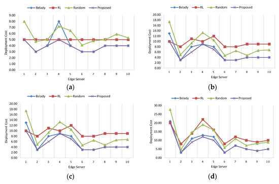
Figure 3. The results of deployment costs for the homogeneous configuration. (a) Number of request: 5; (b) Number of request: 10; (c) Number of request: 15; (d) Number of request: 20.

When the number of requests is 10 (Figure 3b), the result of the proposed method is comparable to Belady, but our method is better than Belady’s approach. The worst performance can be found in the retrospective download with the least recently used. The reason is that the retrospective download with the least recently used method requires some aging time since it utilizes the history information for previous requests. When the numbers of requests are 15 and 20 (Figure 3c,d), the performance ranking is the same as the previous experiment. The total costs for the homogeneous configuration are about 252, 382, 367, and 232, when the Belady, retrospective download with least recently used, random, and the proposed method are used, respectively. The cost of the proposed resource consolidation algorithm for the homogeneous configuration is about 61% over the retrospective download with least recently used, which indicates that our proposed technique effectively reduces the deployment cost.

Figure 4 shows the results of deployment costs for the heterogeneous configuration. When the number of requests is 5 (Figure 4a), the deployment cost for the proposed method outperforms the other three approaches. The total cost of the proposed resource consolidation algorithm is 40, while those of the Belady, retrospective download with least recently used, and random approaches are about 42, 50, and 59.6, respectively. When the number of requests is 10 (Figure 4b), the result of the proposed method also outperforms the Belady, retrospective download with least recently used, and random approaches.

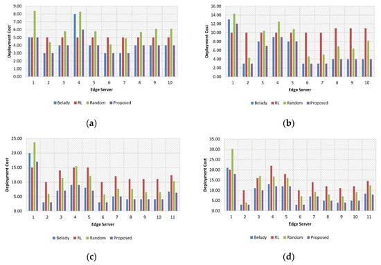
Figure 4. The results of deployment costs for the heterogeneous configuration. (a) Number of request: 5; (b) Number of request: 10; (c) Number of request: 15; (d) Number of request: 20.

When the numbers of requests are 15 and 20 (Figure 4c,d), the top performance can be found in the proposed method, followed by the Belady, random, and retrospective download with least recently used approaches. The total costs for the heterogeneous configuration are about 260, 436, 382, and 246, when the Belady, retrospective download with least recently used, random, and the proposed method are used, respectively. The cost of the proposed resource consolidation algorithm for the heterogeneous configuration is about 56% over the retrospective download, with the least recently used.

In terms of load balance, we measure the standard deviation for the four approaches. More specifically, we sum up the standard deviations for the homogeneous configurations when the numbers of requests are 5, 10, 15, and 20. The results of the values are 5.50, 4.74, 6.77, and 5.00 for the Belady, retrospective download with least recently used, random, and proposed approaches, respectively. The lowest value can be found in the retrospective download with least recently used method, where the performance for the deployment cost is the worst.

The proposed method is second to none in terms of the standard deviation. The reason our resource consolidation algorithm is based on the hidden Markov model is because our method is able to accurately determine whether it uses the edge servers or not by considering the status of mobile devices in nanoscale computing environments. To sum up, our resource consolidation algorithm offers cost efficiency while providing the load balance in nanoscale computing environments.

5. Conclusions

In this paper, we proposed an intelligent and cost-efficient resource consolidation algorithm in nanoscale computing environments, aimed at intelligently choosing the scheduling policy for request and service allocations (either edge servers or the central cloud server) to reduce the responsiveness and the turnaround time while supporting real-time mobile applications. The proposed resource consolidation algorithm is based on the hidden Markov model, one of the artificial intelligence techniques that execute a parameter learning task given the probability model. The proposed algorithm showed that it is capable of reducing the deployment cost for real-time mobile applications or services and achieving the load balance in the cloud system. The costs of the proposed resource consolidation algorithm for the homogeneous and homogeneous configurations are about 61% and 56%, respectively, in comparison with the existing method.

References

- Miraz, M.H.; Ali, M.; Excell, P.S.; Picking, R. Internet of Nano-Things, Things and Everything: Future Growth Trends. Future Internet 2018, 10, 68. [Google Scholar] [CrossRef]
- Pramanik, P.K.D.; Solanki, A.; Debnath, A.; Nayyar, A.; El-Sappagh, S.; Kwak, K. Advancing Modern Healthcare With Nanotechnology, Nanobiosensors, and Internet of Nano Things: Taxonomies, Applications, Architecture, and Challenges. IEEE Access 2020, 8, 65230–65266. [Google Scholar] [CrossRef]
- Fouad, H.; Hashem, M.; Youssef, A.E. A Nano-biosensors model with optimized bio-cyber communication system based on Internet of Bio-Nano Things for thrombosis prediction. J. Nanopart. Res. 2020, 22, 177. [Google Scholar] [CrossRef]
- Buyya, R.; Dastjerdi, A.V. Internet of Things: Principles and Paradigms; Morgan Kaufmann Publishers Inc.: Burlington, MA, USA, 2016; p. 378. [Google Scholar]
- Hassan, N.; Chou, C.T.; Hassan, M. eNEUTRAL IoNT: Energy-Neutral Event Monitoring for Internet of Nano Things. IEEE Internet Things J. 2019, 6, 2379–2389. [Google Scholar] [CrossRef]
- Sicari, S.; Rizzardi, A.; Piro, G.; Coen-Porisini, A.; Grieco, L.A. Beyond the smart things: Towards the definition and the performance assessment of a secure architecture for the Internet of Nano-Things. Comput. Netw. 2019, 162, 106856. [Google Scholar] [CrossRef]
- Wang, D.; Huang, Q.; Chen, X.; Ji, L. Location of three-dimensional movement for a human using a wearable multi-node instrument implemented by wireless body area networks. Comput. Commun. 2020, 153, 34–41. [Google Scholar] [CrossRef]
- Gardašević, G.; Katzis, K.; Bajić, D.; Berbakov, L. Emerging Wireless Sensor Networks and Internet of Things Technologies—Foundations of Smart Healthcare. Sensors 2020, 20, 3619. [Google Scholar] [CrossRef]
- Elazhary, H. Internet of Things (IoT), mobile cloud, cloudlet, mobile IoT, IoT cloud, fog, mobile edge, and edge emerging computing paradigms: Disambiguation and research directions. J. Netw. Comput. Appl. 2019, 128, 105–140. [Google Scholar] [CrossRef]
- Oteafy, S.M.A.; Hassanein, H.S. Leveraging Tactile Internet Cognizance and Operation via IoT and Edge Technologies. Proc. IEEE 2019, 107, 364–375. [Google Scholar] [CrossRef]
- Masdari, M.; Khoshnevis, A. A survey and classification of the workload forecasting methods in cloud computing. Clust. Comput. 2019. [Google Scholar] [CrossRef]
- Jyoti, A.; Shrimali, M. Dynamic provisioning of resources based on load balancing and service broker policy in cloud computing. Clust. Comput. 2020, 23, 377–395. [Google Scholar] [CrossRef]
- Fine, S.; Singer, Y.; Tishby, N. The Hierarchical Hidden Markov Model: Analysis and Applications. Mach. Learn. 1998, 32, 41–62. [Google Scholar] [CrossRef]
- Baum, L.E.; Petrie, T. Statistical Inference for Probabilistic Functions of Finite State Markov Chains. Ann. Math. Stat. 1966, 37, 1554–1563. [Google Scholar] [CrossRef]
- Baum, L.E.; Petrie, T.; Soules, G.; Weiss, N. A Maximization Technique Occurring in the Statistical Analysis of Probabilistic Functions of Markov Chains. Ann. Math. Stat. 1970, 41, 164–171. [Google Scholar] [CrossRef]
- Moghaddam, S.K.; Buyya, R.; Ramamohanarao, K. Performance-Aware Management of Cloud Resources: A Taxonomy and Future Directions. ACM Comput. Surv. 2019, 52, 84. [Google Scholar] [CrossRef]
- Masdari, M.; Zangakani, M. Green Cloud Computing Using Proactive Virtual Machine Placement: Challenges and Issues. J. Grid Comput. 2019. [Google Scholar] [CrossRef]
- Madeo, D.; Mazumdar, S.; Mocenni, C.; Zingone, R. Evolutionary game for task mapping in resource constrained heterogeneous environments. Future Gener. Comput. Syst. 2020, 108, 762–776. [Google Scholar] [CrossRef]
- Ding, D.; Fan, X.; Zhao, Y.; Kang, K.; Yin, Q.; Zeng, J. Q-learning based dynamic task scheduling for energy-efficient cloud computing. Future Gener. Comput. Syst. 2020, 108, 361–371. [Google Scholar] [CrossRef]
- Bibri, S.E. The IoT for smart sustainable cities of the future: An analytical framework for sensor-based big data applications for environmental sustainability. Sustain. Cities Soc. 2018, 38, 230–253. [Google Scholar] [CrossRef]
- Bouet, M.; Conan, V. Mobile Edge Computing Resources Optimization: A Geo-Clustering Approach. IEEE Trans. Netw. Serv. Manag. 2018, 15, 787–796. [Google Scholar] [CrossRef]
- Wang, J.; Zhao, L.; Liu, J.; Kato, N. Smart Resource Allocation for Mobile Edge Computing: A Deep Reinforcement Learning Approach. IEEE Trans. Emerg. Top. Comput. 2019, 1. [Google Scholar] [CrossRef]
- Chadza, T.; Kyriakopoulos, K.G.; Lambotharan, S. Analysis of hidden Markov model learning algorithms for the detection and prediction of multi-stage network attacks. Future Gener. Comput. Syst. 2020, 108, 636–649. [Google Scholar] [CrossRef]
- Dawkins, J.; Hale, J. A systematic approach to multi-stage network attack analysis. In Proceedings of the Second IEEE International Information Assurance Workshop, Charlotte, NC, USA, 9 April 2004; pp. 48–56. [Google Scholar]
- Strayer, W.T.; Jones, C.E.; Schwartz, B.I.; Mikkelson, J.; Livadas, C. Architecture for multi-stage network attack traceback. In Proceedings of the IEEE Conference on Local Computer Networks 30th Anniversary (LCN’05)l, Sydney, NSW, Australia, 17 November 2005; pp. 776–785. [Google Scholar]
- Belady, L.A. A study of replacement algorithms for a virtual-storage computer. IBM Syst. J. 1966, 5, 78–101. [Google Scholar] [CrossRef]
- Hou, I.-H.; Zhao, T.; Wang, S.; Chan, K. Asymptotically optimal algorithm for online reconfiguration of edge-clouds. In Proceedings of the 17th ACM International Symposium on Mobile Ad Hoc Networking and Computing, Paderborn, Germany, 5–8 July 2016; pp. 291–300. [Google Scholar]
© 2020 by the authors. Licensee MDPI, Basel, Switzerland. This article is an open access article distributed under the terms and conditions of the Creative Commons Attribution (CC BY) license (http://creativecommons.org/licenses/by/4.0/).