Deep Neural Network and Long Short-Term Memory for Electric Power Load Forecasting
Abstract
1. Introduction
- (1)
- The peak load approach is used to find the trend curve obtained by plotting the past values of the annual peaks against the years of operation.
- (2)
- The energy approach aims to forecast annual sales, including annual energy sales, to different classes of customers (e.g., residential, commercial, industrial), which can then be converted to the annual peak demand using the annual load factors.
- (1)
- White box-based approaches, also named “physics-based models” require detailed physical information of complex buildings [9,10]. Owing to these characteristics, although the forecasting accuracy is high, a high computational cost is required for the simulation. Recently, there have been a series of attempts to simplify white box-based approaches. However, this simplification is prone to errors and generally overestimates the energy savings of buildings [11,12,13]. There are several tools, such as DOE-2, EnergyPlus, BLAST, TRYSYS, and ESP-r, which aid white box-based approach [14].
- (2)
- Black box-based approaches are also commonly referred to as “data-driven models”. These approaches rely on time-series statistical analyses and machine learning to assess and forecast electricity consumption [15,16,17]. Data-driven models are divided into three categories:
- Conventional models refer to exponential smoothing (ES) [18], moving average (MA) [19], statistical regressions [20], auto-regressive (AR) models [21], genetic algorithms (GA) [22], and fuzzy-based models [23,24]. They provide a good balance between forecasting accuracy and implementation simplicity. However, they have shown significant limitations in their ability to model nonlinear data patterns and the forecasting horizon.
- Artificial intelligence models have been studied for many years and are generally referred to as machine learning and deep learning [27]. Some of the most popular artificial intelligence models are support vector machine (SVM) [28], artificial neural networks (ANN) [29], deep neural network (DNN) [30], and long short-term memory (LSTM) [31]. These models-based forecasting algorithms lead to less operator-dependent and more versatile methods in terms of data usage, with much higher forecasting accuracy.
- (3)
- Grey-box-based approaches have also been named “hybrid-based models” which are a combination of white box and black box models [32,33,34,35]. These models have the advantage of using improved single data-driven models with optimization, or a combination of several machine learning algorithms. However, these approaches have the shortcoming of computational inefficiency because these approaches involve uncertain inputs and complex interactions among elements and stochastic occupant behaviors [36,37,38].
2. Preliminaries and Problem Definition
2.1. Load Forecasting
- (1)
- The advantages of load forecasting are as follows:
- It helps utility companies to better operate and manage supplies for their customers;
- It is an important process that can increase the efficiency and profit of power generation and distribution companies.
- (2)
- The challenges of load forecasting are as follows:
- The power load series is complex and shows various seasonality levels; hence, a given time load can be accommodated at the same time in a specific weekday for the same time load and the previous week as well as the previous time load;
- (1)
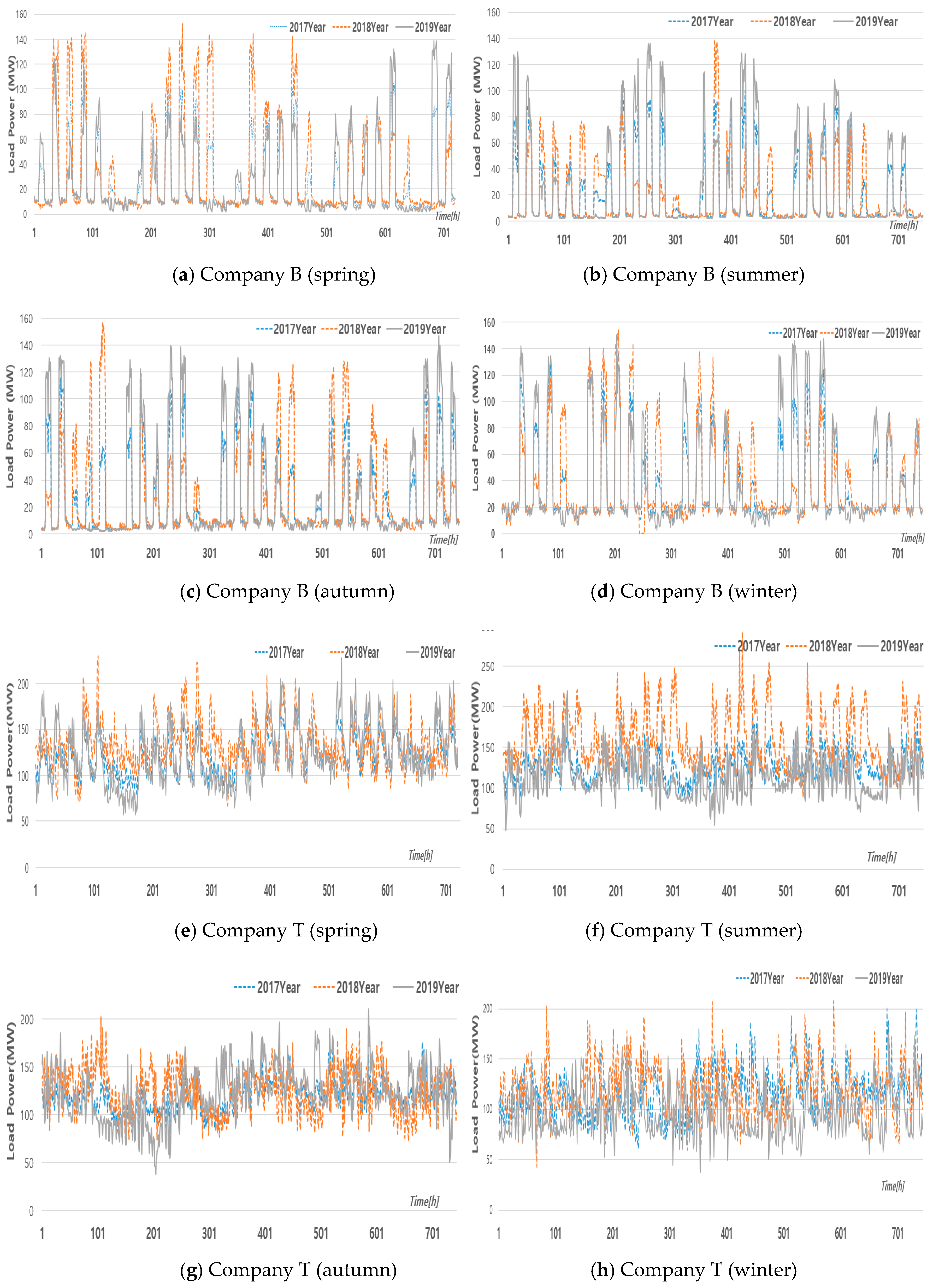
- The electricity usage of company B for three years is in the order of summer (121 MW) < spring (154 MW) < autumn (159 MW) < winter (197 MW). It is less affected by weather than summer and winter, where air-conditioning usage is the highest.
- (2)
- It showed the highest electricity usage occurs during working hours (8 a.m. to 7 p.m.) from Monday to Friday (weekdays). Saturdays and Sundays (weekends) show that there is almost no electricity usage (below 50 MW). In addition, there was almost no power consumption during lunchtime from 12:00 to 1:00 p.m. compared with other hours on weekdays.
- (3)
- As a result of comparing the electricity usage for special days of company B for three years, the power consumption pattern is regular in April and July because there are no special holidays. In addition, in October, as special holidays are mostly from Monday to Friday, power consumption patterns are regular, similar to those of April and July. However, January had high electricity usage on Wednesdays and Thursdays, excluding special holidays (Monday, Tuesday, and Friday).
- (1)
- The electricity usage of T company for three years is in the order of winter (488 MW) < spring (511 MW) < autumn (546 MW) < summer (605 MW). As company T is a livestock meat processing company, cooling is more important than heating, so it uses more electricity in spring, autumn, and summer than in winter.
- (2)
- The power consumption pattern of company T’s weekend (Saturday to Sunday) is smaller than on weekdays, but fluctuations in electricity usage are more flexible at each time than those of company B. In particular, the power consumption pattern during the week largely fluctuates regardless of the time of day and day of the week.
- (3)
- As a result of comparing the electricity power for special days at company T for three years, it can be seen that the electricity usage of company T differs depending on the amount of supply, regardless of the special days.
2.2. DNN
2.3. LSTM
3. Proposed Electric Power Load Forecasting Methodology
3.1. Proposed Multivariate Model
3.2. Proposed DNN Model
3.3. Proposed LSTM Model
3.4. Simulation Parameters of the DNN and LSTM
4. Case Studies and Discussion
4.1. Test Environment and Test Data Set
4.2. Performance Evaluation Metrics
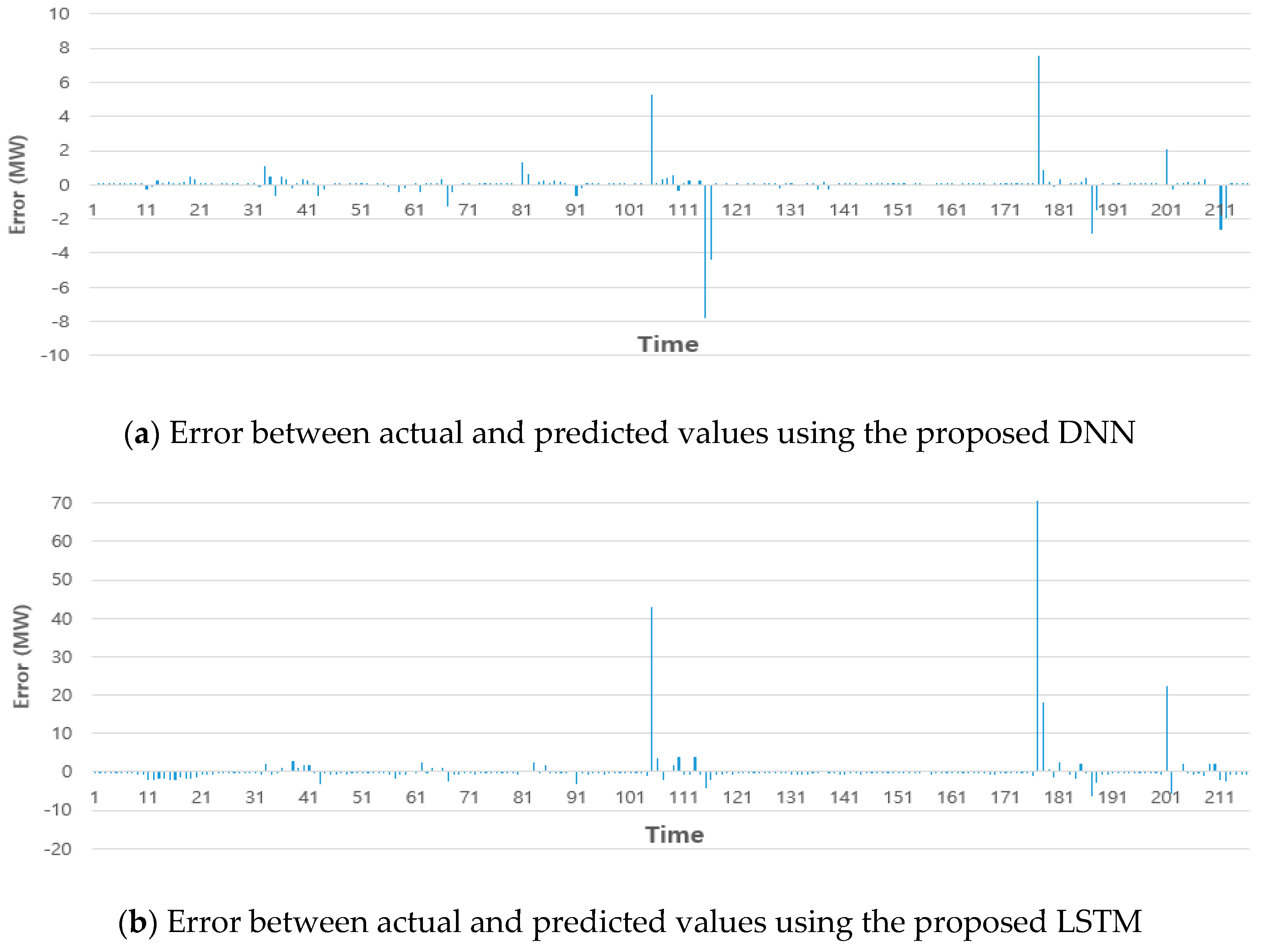
4.3. Comparison and Analysis of Medium-Term Electric Power Load Forecasting
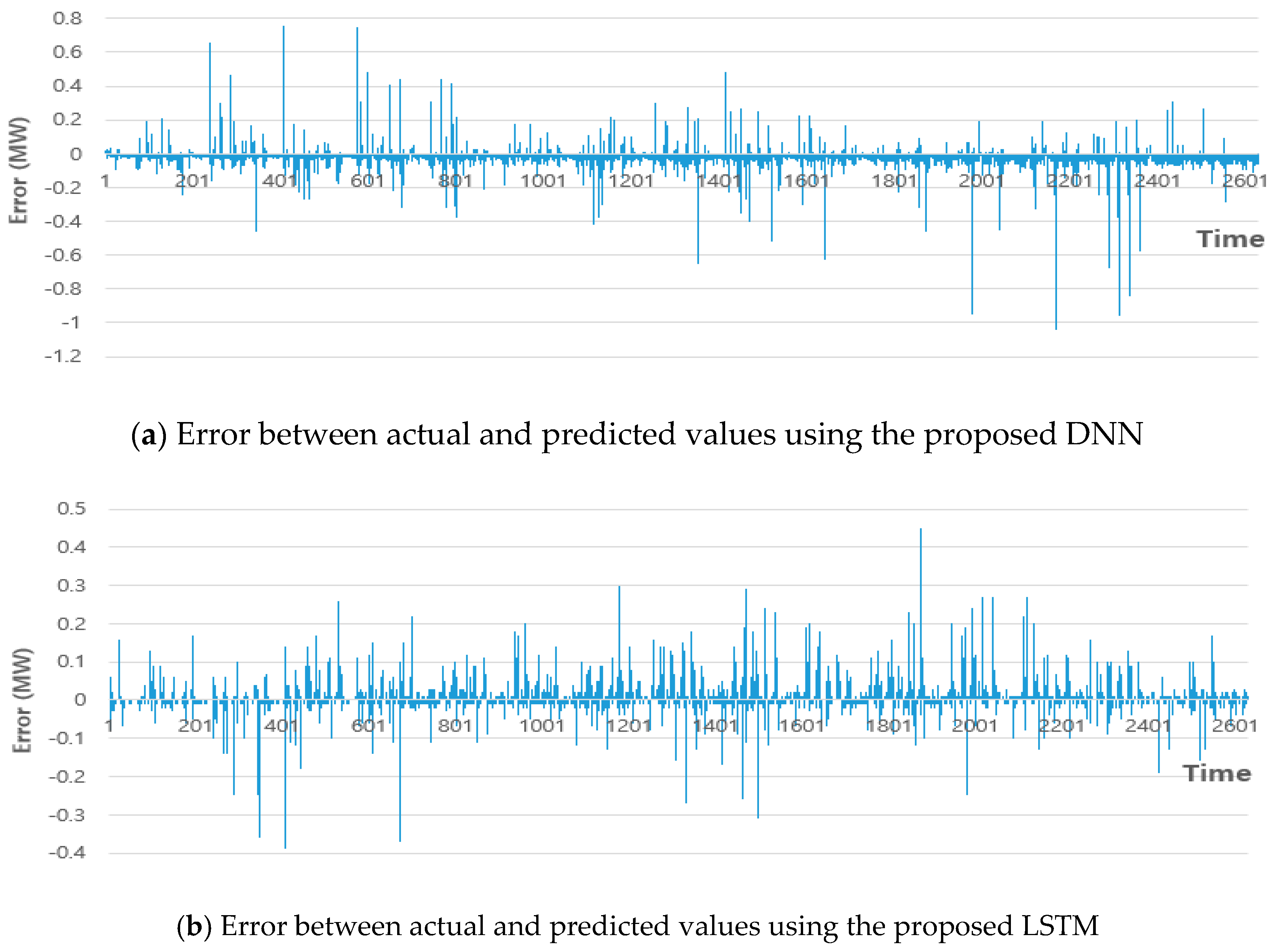
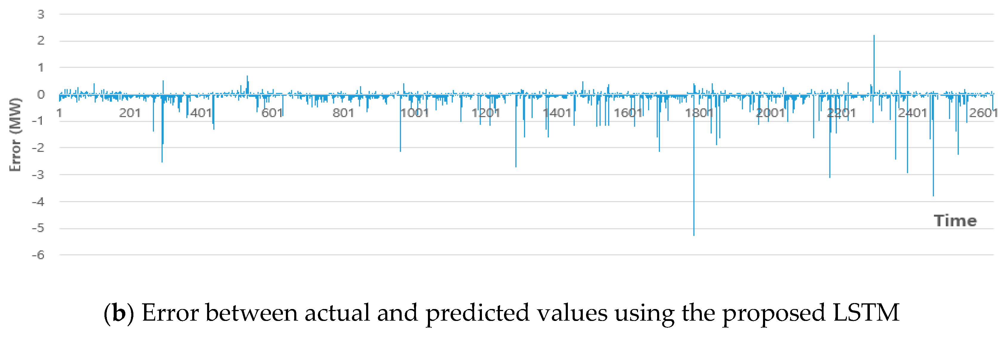
4.4. Comparison and Analysis of Long-Term Electric Power Load Forecasting
5. Conclusions and Future Work
Author Contributions
Funding
Acknowledgments
Conflicts of Interest
References
- Almeshaiei, A.; Soltan, H. A methodology for electric power load forecasting. Alex. Eng. J. 2011, 50, 137–144. [Google Scholar] [CrossRef]
- Yu, C.-N.; Mirowski, P.; Ho, T.K. A sparse coding approach to household electricity demand forecasting in smart grids. IEEE Trans. Smart Grid 2017, 8, 738–748. [Google Scholar] [CrossRef]
- Zheng, S.; Zhong, Q.; Peng, L.; Chai, X. A simple method of residential electricity load forecasting by improved Bayesian neural networks. Hindawi Math. Probl. Eng. 2018, 2018, 4276176. [Google Scholar] [CrossRef]
- Al-Hamadi, H.M.; Soliman, A. Long-term/mid-term electric load forecasting based on short-term correlation and annual growth. Electr. Power Syst. Res. 2005, 74, 353–361. [Google Scholar] [CrossRef]
- Feng, Y. Study on Medium and Long Term Power Load Forecasting Based on Combination Forecasting Model. Chem. Eng. Trans. 2015, 51, 859–864. [Google Scholar]
- Xue, B.; Keng, J. Dynamic transverse correction method of middle and long term energy forecasting based on statistic of forecasting errors. In Proceedings of the Conference on Power and Energy IPEC, Ho Chi Minh City, Vietnam, 12–14 December 2012; pp. 253–256. [Google Scholar]
- Wei, Y.; Zhang, X.; Shi, Y.; Xia, L.; Pan, S.; Wu, J.; Han, M.; Zhao, X. A review of data-driven approaches for prediction and classification of building energy consumption. Renew. Sustain. Energy Rev. 2018, 82, 1027–1047. [Google Scholar] [CrossRef]
- Bourdeau, M.; Zhai, X.Q.; Nefzaoui, E.; Guo, X.; Chatellier, P. Modeling and forecasting building energy consumption: A review of data-driven techniques. Sustain. Cities Soc. 2019, 48, 101533. [Google Scholar] [CrossRef]
- Yildiz, B.; Bilbao, J.I.; Sproul, A.B. A review and analysis of regression and machine learning models on commercial building electricity load forecasting. Renew. Sustain. Energy Rev. 2017, 73, 1104–1122. [Google Scholar] [CrossRef]
- Boris, D.; Milan, V.; Milos, Z.J.; Milija, S. White-Box or Black-Box Decision Tree Algorithms: Which to Use in Education? IEEE Trans. Educ. 2013, 56, 287–291. [Google Scholar] [CrossRef]
- Cavalheiro, J.; Carreira, P. A multidimensional data model design for building energy management. Adv. Eng. Inform. 2016, 30, 619–632. [Google Scholar] [CrossRef]
- Al-Homoud, M.S. Computer-aided building energy analysis techniques. Build. Environ. 2001, 36, 421–433. [Google Scholar] [CrossRef]
- Barnaby, C.S.; Spitler, J.D. Development of the residential load factor method for heating and cooling load calculations. ASHRAE Trans. 2005, 111, 291–307. [Google Scholar]
- Building Energy Software Tool. Available online: https://www.buildingenergysoftwaretools.com/ (accessed on 7 March 2020).
- Zhao, H.X.; Magoulès, F. A review on the prediction of building energy consumption. Renew. Sustain. Energy Rev. 2012, 16, 3586–3592. [Google Scholar] [CrossRef]
- Williams, S.; Short, M. Electricity demand forecasting for decentralised energy management. Energy Build. Environ. 2020, 1, 178–186. [Google Scholar] [CrossRef]
- González-Vidal, A.; Ramallo-González, A.P.; Terroso-Sáenz, F.; Skarmeta, A. Data driven modeling for energy consumption prediction in smart building. In Proceedings of the 2017 IEEE International Conference on Big Data, Boston, MA, USA, 11–14 December 2017; IEEE: New York, NY, USA, 2017. [Google Scholar]
- Brown, R.G. Smoothing Forecasting and Prediction of Discrete Time Series; Prentice-Hall: Englewood Cliffs, NJ, USA, 1963. [Google Scholar]
- Simple Moving Average. Available online: https://www.investopedia.com/terms/s/sma.asp (accessed on 7 March 2020).
- Holt, C.E. Forecasting Seasonal and Trends by Exponentially Weighted Average (O.N.R. Memorandum No. 52); Carnegie Institute of Technology: Pittsburgh, PA, USA, 1957. [Google Scholar]
- Ohtsuka, Y.; Oga, T.; Kakamu, K. Forecasting electricity demand in Japan: A Bayesian spatial autoregressive ARMA approach. Comp. Stat. Data Anal. 2010, 54, 2721–2735. [Google Scholar] [CrossRef]
- Kubota, N.; Hashimoto, S.; Kojima, F.; Taniguchi, K. GP-preprocessed fuzzy inference for the energy load prediction. In Proceedings of the 2000 Congress on Evolutionary Computation, La Jolla, CA, USA, 16–19 July 2000; IEEE: New York, NY, USA, 2000; Volume 1, pp. 1–6. [Google Scholar]
- Song, Q.; Chissom, B.S. Fuzzy time series and its models. Fuzzy Sets Syst. 1993, 54, 269–277. [Google Scholar] [CrossRef]
- Jallala, M.A.; González-Vidal, A.; Skarmeta, A.F.; Chabaa, S.; Zeroual, A. A hybrid neuro-fuzzy inference system-based algorithm for time series forecasting is applied to energy consumption prediction. Appl. Energy 2020, 268, 114977. [Google Scholar] [CrossRef]
- Fix, E.; Hodges, J.L., Jr. Discriminatory Analysis—Nonparametric Discrimination: Consistency Properties; International Statistical Institute: Voorburg, The Netherlands, 1989; Volume 57, pp. 238–247. [Google Scholar]
- Yu, Z.; Haghighat, F.; Fung, B.C.M.; Yoshino, H. A decision tree method for building energy demand modeling. Energy Build. 2010, 42, 1637–1646. [Google Scholar] [CrossRef]
- Liu, T.; Tan, Z.; Xu, C.; Chen, H.; Li, Z. Study on deep reinforcement learning techniques for building energy consumption forecasting. Energy Build. 2020, 208, 109675. [Google Scholar] [CrossRef]
- Dong, B.; Cao, C.; Lee, S.E. Applying support vector machines to predict building energy consumption in tropical region. Energy Build. 2005, 37, 545–553. [Google Scholar] [CrossRef]
- Kalogirou, S.A.; Neocleous, C.C.; Schizas, C.N. Building heating load estimation using artificial neural networks. In Proceedings of the 17th International Conference on Parallel Architectures and Compilation Techniques, San Francisco, CA, USA, 10–14 November 1997; Association for Computing Machinery: Toronto, ON, Canada, 1997. [Google Scholar]
- Bagnasco, A.; Fresi, F.; Saviozzi, M.; Silvestro, F.; Vinci, A. Electrical consumption forecasting in hospital facilities: An application case. Energy Build. 2015, 103, 261–270. [Google Scholar] [CrossRef]
- Gers, F.; Schmidhuber, J.; Cummins, F. Learning to Forget: Continual Prediction with LSTM. In Proceedings of the 9th International Conference on Artificial Neural Networks, ICANN’99, Edinburgh, UK, 7–10 September 1999; pp. 850–855. [Google Scholar]
- Foucquier, A.; Robert, S.; Suard, F.; Stéphan, L.; Jay, A. State of the art in building modelling and energy performances prediction: A review. Renew. Sustain. Energy Rev. 2013, 23, 272–288. [Google Scholar] [CrossRef]
- Tardioli, G.; Kerrigan, R.; Oates, M.; O’Donnell, J.; Finn, D. Data driven approaches for prediction of building energy consumption at urban level. Energy Proc. 2015, 78, 3378–3383. [Google Scholar] [CrossRef]
- Chalal, M.L.; Benachir, M.; White, M.; Shrahily, R. Energy planning and forecasting approaches for supporting physical improvement strategies in the building sector: A review. Renew. Sustain. Energy Rev. 2016, 64, 761–776. [Google Scholar] [CrossRef]
- Mat Daut, M.A.; Hassan, M.Y.; Abdullah, H.; Rahman, H.A.; Abdullah, M.P.; Hussin, F. Building electrical energy consumption forecasting analysis using conventional and artificial intelligence methods: A review. Renew. Sustain. Energy Rev. 2017, 70, 1108–1118. [Google Scholar] [CrossRef]
- Paudel, S.; Nguyen, P.H.; Kling, W.L.; Elmitri, M.; Lacarrière, B.; Corre, O.L. Support vector machine in prediction of building energy demand using pseudo dynamic approach. In Proceedings of the ECOS 2015—The 28th International Conference on Efficiency, Cost, Optimization, Simulation and Environmental Impact of Energy Systems, Pau, France, 30 June 2015. [Google Scholar]
- Li, Z.; Han, Y.; Xu, P. Methods for benchmarking building energy consumption against its past or intended performance: An overview. Appl. Energy 2014, 124, 325–334. [Google Scholar] [CrossRef]
- Diamantoulakis, P.D.; Kapinas, V.M.; Karagiannidis, G.K. Big data analytics for dynamic energy management in smart grids. Big Data Res. 2015, 5, 94–101. [Google Scholar] [CrossRef]
- Raza, M.Q.; Khosravi, A. A review on artificial intelligence based load demand forecasting techniques for smart grid and buildings. Renew. Sustain. Energy Rev. 2015, 50, 1352–1372. [Google Scholar] [CrossRef]
- Suganthi, L.; Samuel, A.A. Energy models for demand forecasting—A review. Renew. Sustain. Energy Rev. 2012, 16, 1223–1240. [Google Scholar] [CrossRef]
- Wang, Z.; Jun, L.; Zhu, S.; Zhao, J.; Deng, S.; Zhong, S.; Yin, H.; Li, H.; Qi, Y.; Gan, Z. A review of load forecasting of the distributed energy system. IOP Conf. Ser. Earth Environ. Sci. 2019, 237, 042019. [Google Scholar] [CrossRef]
- Shao, Z.; Gao, F.; Zhang, Q.; Yang, S.L. Multivariate statistical and similarity measure based semiparametric modeling of the probability distribution: A novel approach to the case study of mid-long term electricity consumption forecasting in China. Appl. Energy 2015, 156, 502–518. [Google Scholar] [CrossRef]
- Clements, A.E.; Hurn, A.S.; Li, Z. Forecasting dayahead electricity load using a multiple equation time series approach. Eur. J. Oper. Res. 2016, 251, 522–530. [Google Scholar] [CrossRef]
- De Felice, M.; Alessandri, A.; Catalano, F. Seasonal weather forecasts for medium-term electricity demand forecasting. Appl. Energy 2015, 137, 435–444. [Google Scholar] [CrossRef]
- Khatoon, S.; Sing, A.K. Effects of various factors on electric load forecasting: An overview. In Proceedings of the IEEE Power India International Conference (PIICON), Delhi, India, 5–7 December 2014; pp. 1–5. [Google Scholar]
- Xiao, L.; Shao, W.; Liang, T.; Wang, C. A combined model based on multiple seasonal patterns and modified firefly algorithm for electrical load forecasting. Appl. Energy 2016, 167, 135–153. [Google Scholar] [CrossRef]
- Andersen, F.M.; Larsen, H.V.; Boomsma, T.K. Long-term forecasting of hourly electricity load: Identification of consumption profiles and segmentation of customers. Energy Convers. Manag. 2013, 68, 244–252. [Google Scholar] [CrossRef]
- Sobhani, M.; Campbell, A.; Sangamwar, S.; Li, C.; Hong, T. Combining weather stations for electric load forecasting. Energies 2019, 12, 1510. [Google Scholar] [CrossRef]
- Hastie, T.; Tibshirani, R.; Friedman, J. The Elements of Statistical Learning: Data Mining, Inference, and Prediction; Springer: New York, NY, USA, 2009. [Google Scholar]
- Hochreiter, S.; Schmidhuber, J. Long short-term memory. Neural Comput. 1997, 9, 1735–1780. [Google Scholar] [CrossRef] [PubMed]
- Li, D.; Yu, D. Deep learning: Methods and applications. Found. Trends Signal. Process. 2014, 30, 197–387. [Google Scholar]
- Lecun, Y. Gradient-based learning applied to document recognition. Proc. IEEE 1998, 86, 2278–2324. [Google Scholar] [CrossRef]
- Sainath, T.; Mohamed, A.R.; Kingsbury, B.; Ramabhadran, B. Convolutional neural networks for LVCSR. IEEE ICASSP 2013. [Google Scholar] [CrossRef]
- Mocanu, E.; Nguyen, P.H.; Gibescu, M.; Kling, W.L. Deep learning for estimating building energy consumption. Sustain. Energy Grids Netw. 2016, 6, 91–99. [Google Scholar] [CrossRef]
- Cho, K.; van Merrienboer, B.; Gulcehre, C.; Bahdanau, D.; Bougares, F.; Schwenk, H.; Bengio, Y. Learning Phrase Representations Using RNN Encoder–Decoder for Statistical Machine Translation. EMNLP 2014. [Google Scholar] [CrossRef]
- Hochreiter, S.; Bengio, Y.; Paolo, F.; Schmidhuber, J. Gradient Flow in Recurrent Nets: The Difficulty of Learning Long-Term Dependencies; IEEE Press: Los Alamitos, CA, USA, 2001; pp. 237–243. [Google Scholar]
- Keras.io: The Python Deep Learning Library. Available online: https://keras.io/ (accessed on 7 March 2020).
- Kingma, D.; Ba, J. Adam: A method for stochastic optimization. In Proceedings of the International Conference on Learning Representations, ICLR, San Diego, CA, USA, 7–9 May 2015; pp. 1–15. [Google Scholar]
- Nair, V.; Hinton, G. Rectified linear units improve restricted Boltzmann machines. In Proceedings of the International Conference on Machine Learning, ICML, Haifa, Israel, 21–24 June 2010; pp. 807–814. [Google Scholar]
- Tensorflow.org: Deep Learning Library Developed by Google. Available online: https://www.tensorflow.org/ (accessed on 7 March 2020).
- Hong, T.; Kim, J.; Koo, C. LCC and LCCO2 analysis of green roofs in elementary schools with energy saving measures. Energy Build. 2012, 45, 229–239. [Google Scholar] [CrossRef]


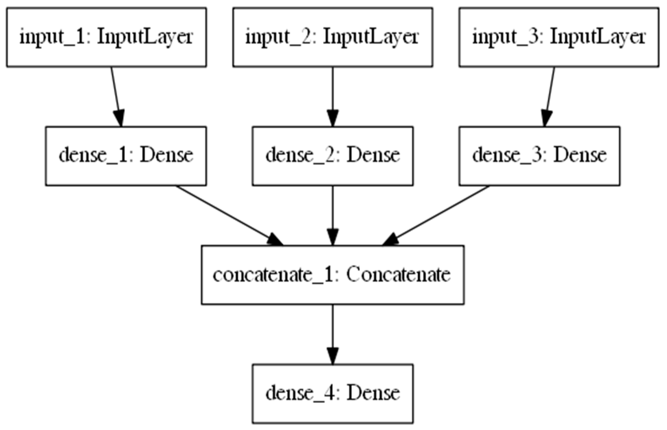
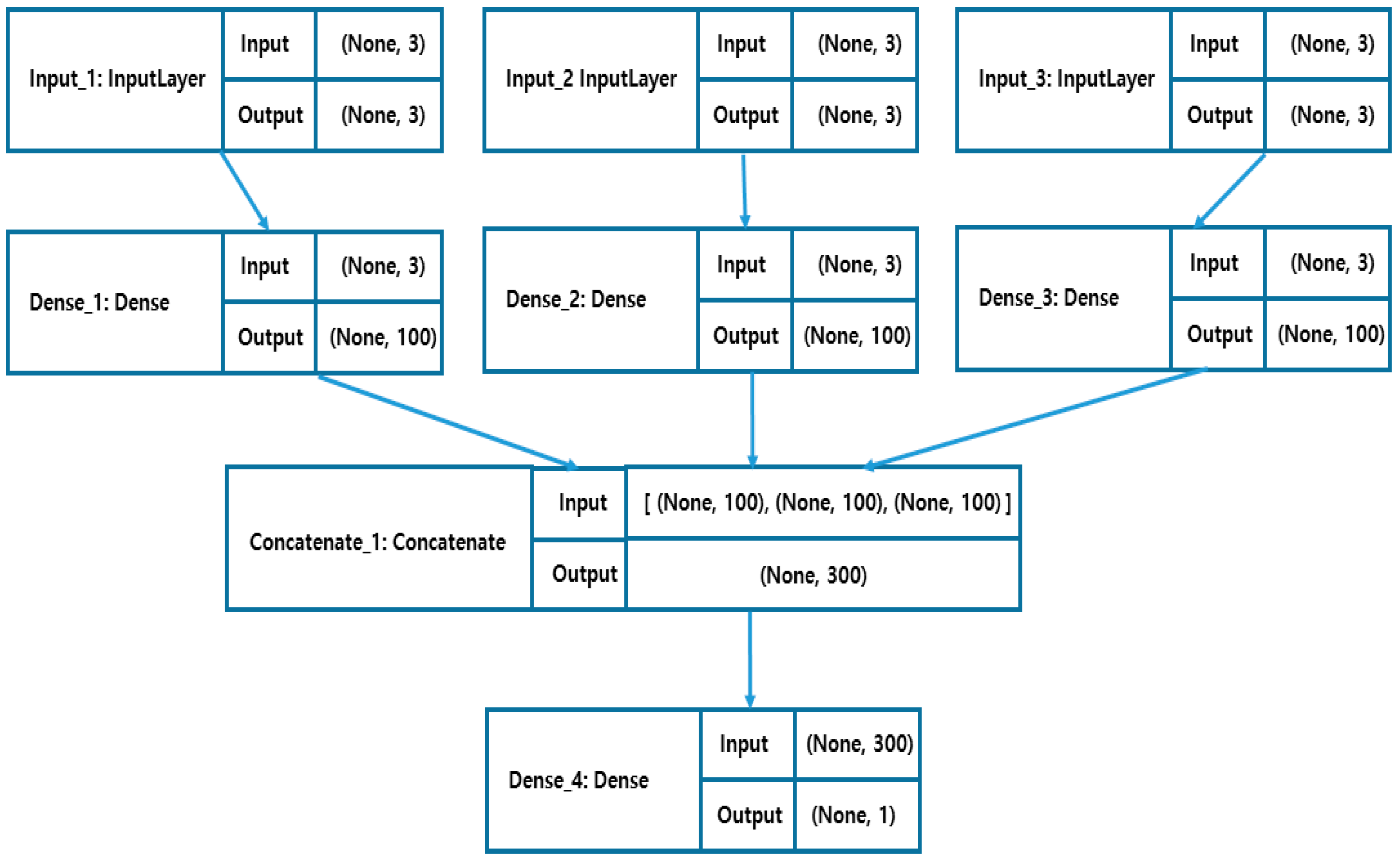
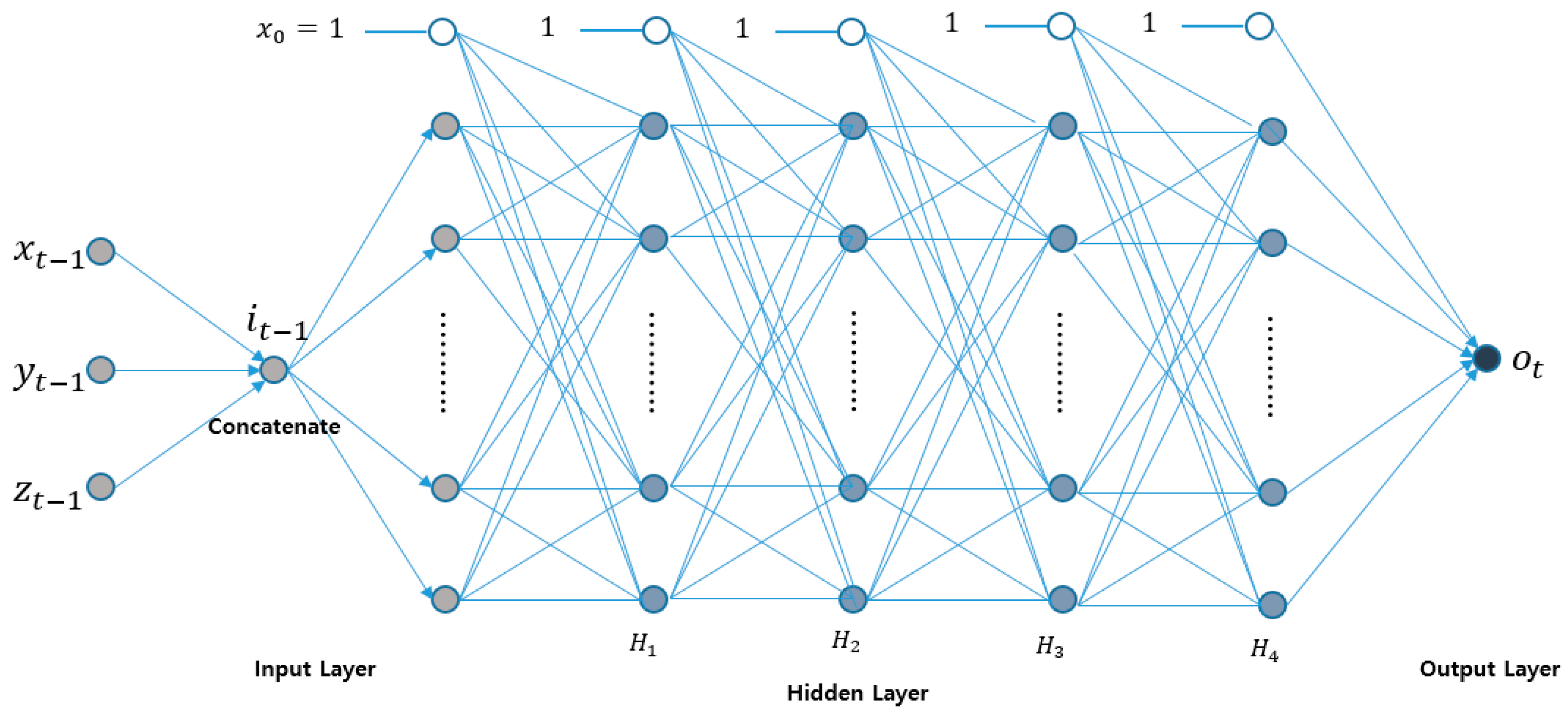
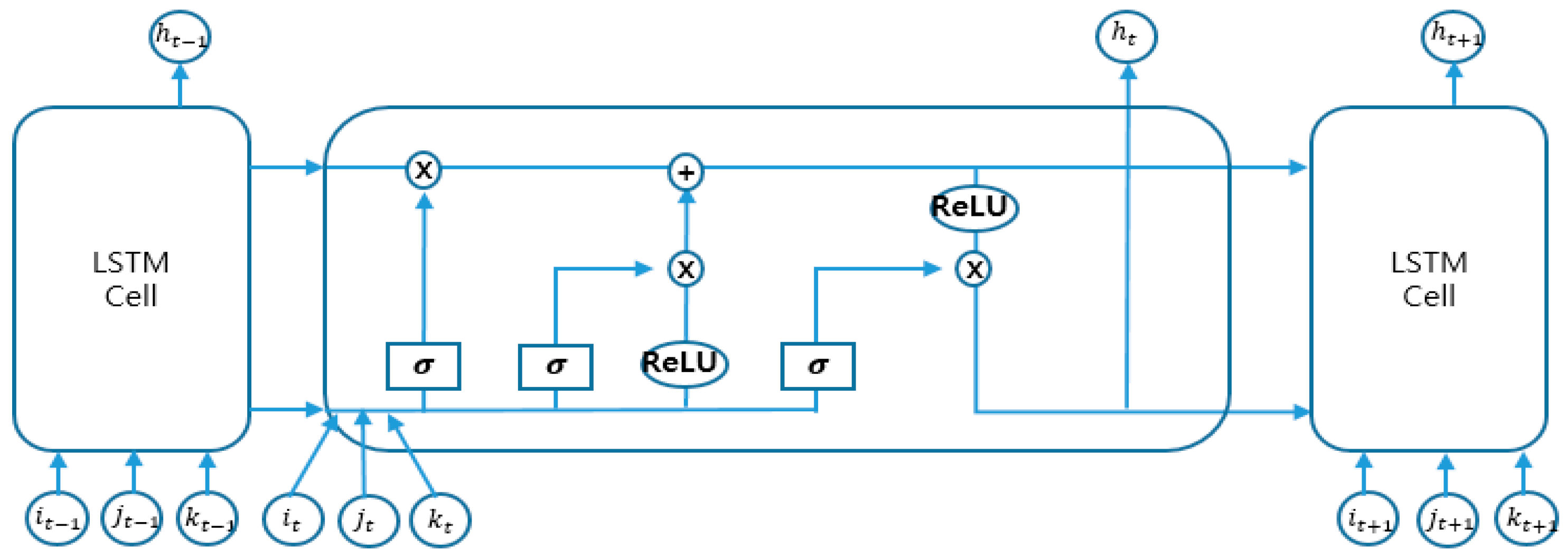


| Year | January | April | July | Autumn |
|---|---|---|---|---|
| 2017 | 1/1(Tuesday), 1/27(Friday)–1/30(Monday) | X | X | 10/1(Sunday)–10/9(Monday) |
| 2018 | 1/1(Monday) | X | X | 10/3(Wednesday), 10/9(Tuesday) |
| 2019 | 1/1(Tuesday) | X | X | 10/3(Thursday), 10/9(Wednesday) |
| Parameter | DNN | LSTM |
|---|---|---|
| Number of layers | 4 | 2 |
| Number of neurons | 100 | 100 |
| Number of epochs | 10 | 10 |
| Learning rate | 0.05 | 0.05 |
| Loss function | MSE | MSE |
| Optimizer | ADAM | ADAM |
| Weight initializer | 1 | 1 |
| Activation function | ReLU | ReLU |
| Term | Training Set | Testing Set | ||
|---|---|---|---|---|
| From | To | From | To | |
| MTLF | ||||
| 1 January 2019 | 22 January 2019 | 23 January 2019 | 31 January 2019 | |
| 1 February 2019 | 20 February 2019 | 21 February 2019 | 29 February 2019 | |
| 1 March 2019 | 22 March 2019 | 23 March 2019 | 31 March 2019 | |
| 1 April 2019 | 21 April 2019 | 22 April 2019 | 30 April 2019 | |
| 1 May 2019 | 22 May 2019 | 23 May 2019 | 31 May 2019 | |
| 1 June 2019 | 21 June 2019 | 22 June 2019 | 30 June 2019 | |
| 1 July 2019 | 22 July 2019 | 23 July 2019 | 31 July 2019 | |
| 1 August 2019 | 22 August 2019 | 23 August 2019 | 31 August 2019 | |
| 1 September 2019 | 21 September 2019 | 22 September 2019 | 30 September 2019 | |
| 1 October 2019 | 22 October 2019 | 23 October 2019 | 31 October 2019 | |
| 1 November 2019 | 21 November 2019 | 22 November 2019 | 30 November 2019 | |
| 1 December 2019 | 22 Dec. 2019 | 23 Dec. 2019 | 31 December 2019 | |
| LTLF | ||||
| 1 January 2019 | 13 September 2019 | 14 September 2019 | 31 December 2019 |
| Month | Metrics | Company B | Company T | Δ | |||||
|---|---|---|---|---|---|---|---|---|---|
| DNN (A) | LSTM (B) | ΔB (A–B) | DNN (C) | LSTM (D) | ΔT (C–D) | ΔDNN (A–C) | ΔLSTM (B–D) | ||
| January | MAE(MW) | 0.15 | 0.43 | −0.28 | 0.19 | 1.09 | −0.90 | −0.66 | −0.04 |
| RMSE(MW) | 0.30 | 0.97 | −0.67 | 0.26 | 1.75 | −1.49 | −0.78 | 0.04 | |
| CVRMSE(%) | 0.73 | 2.37 | −1.64 | 0.21 | 1.44 | −1.23 | 0.93 | 0.52 | |
| MAPE (%) | 0.58 | 0.94 | −0.36 | 0.16 | 0.88 | −0.72 | 0.06 | 0.42 | |
| R2 | 0.99 | 0.99 | 0 | 0.99 | 0.99 | 0 | 0 | 0 | |
| Time (ms) | 1.37 | 4.17 | −2.80 | 1.64 | 4.28 | −2.64 | −0.11 | −0.27 | |
| February | MAE(MW) | 0.15 | 0.78 | −0.63 | 0.13 | 1.02 | −0.89 | −0.24 | 0.02 |
| RMSE(MW) | 0.35 | 2.37 | −2.02 | 0.28 | 1.67 | −1.39 | 0.70 | 0.07 | |
| CVRMSE(%) | 0.81 | 5.49 | −4.68 | 0.23 | 1.37 | −1.14 | 4.12 | 0.58 | |
| MAPE (%) | 0.67 | 2.49 | −1.82 | 0.10 | 0.77 | −0.67 | 1.72 | 0.57 | |
| R2 | 0.99 | 0.99 | 0 | 0.99 | 0.99 | 0 | 0 | 0 | |
| Time (ms) | 1.34 | 3.73 | −2.39 | 1.51 | 4.43 | −2.92 | −0.70 | −0.17 | |
| March | MAE(MW) | 0.20 | 0.80 | −0.60 | 0.21 | 1.47 | −1.26 | −0.67 | −0.01 |
| RMSE(MW) | 0.49 | 1.79 | −1.3 | 0.40 | 2.41 | −2.01 | −0.62 | 0.09 | |
| CVRMSE(%) | 1.52 | 5.54 | −4.02 | 0.33 | 1.99 | −1.66 | 3.55 | 1.19 | |
| MAPE (%) | 1.65 | 4.40 | −2.75 | 0.16 | 1.25 | −1.09 | 3.15 | 1.49 | |
| R2 | 0.99 | 0.99 | 0 | 0.99 | 0.99 | 0 | 0 | 0 | |
| Time (ms) | 1.35 | 4.09 | −2.74 | 1.74 | 4.81 | −3.07 | −0.72 | −0.39 | |
| April | MAE(MW) | 0.28 | 1.56 | −1.28 | 0.14 | 0.88 | −0.74 | 0.68 | 0.14 |
| RMSE(MW) | 0.96 | 6.08 | −5.12 | 0.19 | 1.29 | −1.10 | 4.79 | 0.77 | |
| CVRMSE(%) | 3.02 | 19.14 | −16.12 | 0.15 | 1.01 | −0.86 | 18.13 | 2.87 | |
| MAPE (%) | 2.15 | 8.75 | −6.60 | 0.10 | 0.67 | −0.57 | 8.08 | 2.05 | |
| R2 | 0.99 | 0.97 | 0.02 | 0.99 | 0.99 | 0 | −0.02 | 0 | |
| Time (ms) | 1.31 | 3.95 | −2.64 | 1.60 | 4.28 | −2.68 | −0.33 | −0.29 | |
| May | MAE(MW) | 0.10 | 0.87 | −0.77 | 0.20 | 6.60 | −6.40 | −5.73 | −0.10 |
| RMSE(MW) | 0.29 | 2.77 | −2.48 | 0.27 | 9.27 | −9.00 | −6.50 | 0.02 | |
| CVRMSE(%) | 1.05 | 10.05 | −9.00 | 0.17 | 5.68 | −5.51 | 4.37 | 0.88 | |
| MAPE (%) | 2.13 | 8.05 | −5.92 | 0.12 | 4.00 | −3.88 | 4.05 | 2.01 | |
| R2 | 0.99 | 0.99 | 0 | 0.99 | 0.88 | 0.11 | 0.11 | 0 | |
| Time (ms) | 1.42 | 4.12 | −2.70 | 1.74 | 4.62 | −2.88 | −0.50 | −0.32 | |
| June | MAE(MW) | 0.17 | 0.78 | −0.61 | 0.55 | 1.41 | −0.86 | −0.63 | −0.38 |
| RMSE(MW) | 0.32 | 1.52 | −1.20 | 0.69 | 2.02 | −1.33 | −0.50 | −0.37 | |
| CVRMSE(%) | 1.10 | 5.21 | −4.11 | 0.42 | 1.22 | −0.8 | 3.99 | 0.68 | |
| MAPE (%) | 1.90 | 8.38 | −6.48 | 0.34 | 0.82 | −0.48 | 7.56 | 1.56 | |
| R2 | 0.99 | 0.99 | 0 | 0.99 | 0.99 | 0 | 0 | 0 | |
| Time (ms) | 1.36 | 4.28 | −2.92 | 1.62 | 4.43 | −2.81 | −0.15 | −0.26 | |
| July | MAE(MW) | 0.09 | 0.34 | −0.25 | 0.40 | 1.70 | −1.30 | −1.36 | −0.31 |
| RMSE(MW) | 0.19 | 0.62 | −0.43 | 0.53 | 2.53 | −2.00 | −1.91 | −0.34 | |
| CVRMSE(%) | 0.87 | 2.84 | −1.97 | 0.34 | 1.61 | −1.27 | 1.23 | 0.53 | |
| MAPE (%) | 1.12 | 4.04 | −2.92 | 0.25 | 1.07 | −0.82 | 2.97 | 0.87 | |
| R2 | 0.99 | 0.99 | 0 | 0.99 | 0.99 | 0 | 0 | 0 | |
| Time (ms) | 1.43 | 4.17 | −2.74 | 1.65 | 4.63 | −2.98 | −0.46 | −0.22 | |
| August | MAE(MW) | 0.19 | 0.74 | −0.55 | 0.35 | 1.44 | −1.09 | −0.70 | −0.16 |
| RMSE(MW) | 0.43 | 1.92 | −1.49 | 0.48 | 2.47 | −1.99 | −0.55 | −0.55 | |
| CVRMSE(%) | 2.34 | 10.46 | −8.12 | 0.31 | 1.61 | −1.3 | 8.85 | 2.03 | |
| MAPE (%) | 3.42 | 6.27 | −2.85 | 0.22 | 0.94 | −0.72 | 5.33 | 3.20 | |
| R2 | 0.99 | 0.99 | 0 | 0.99 | 0.99 | 0 | 0 | 0 | |
| Time (ms) | 1.37 | 4.75 | −3.38 | 1.67 | 4.71 | −3.04 | 0.04 | −0.30 | |
| September | MAE(MW) | 0.10 | 0.77 | −0.67 | 0.27 | 2.97 | −2.67 | −2.17 | −0.17 |
| RMSE(MW) | 0.21 | 2.46 | −2.25 | 0.76 | 4.90 | −4.14 | −2.44 | −0.55 | |
| CVRMSE(%) | 0.72 | 8.45 | −7.73 | 4.16 | 0.65 | 3.51 | 7.80 | −3.44 | |
| MAPE (%) | 1.12 | 3.76 | −2.64 | 0.24 | 3.17 | −2.93 | 0.59 | 0.88 | |
| R2 | 0.99 | 0.99 | 0 | 0.99 | 0.95 | 0.04 | 0.04 | 0 | |
| Time (ms) | 1.30 | 3.98 | −2.68 | 1.59 | 4.60 | −3.01 | −0.62 | −0.29 | |
| October | MAE(MW) | 0.13 | 0.84 | −0.71 | 0.27 | 1.41 | −1.41 | −0.57 | −0.14 |
| RMSE(MW) | 0.24 | 1.39 | −1.15 | 0.43 | 2.20 | −1.77 | −0.81 | −0.19 | |
| CVRMSE(%) | 0.83 | 4.80 | −3.97 | 0.34 | 1.76 | −1.42 | 3.04 | 0.49 | |
| MAPE (%) | 1.01 | 6.81 | −5.80 | 0.22 | 1.17 | −0.95 | 5.64 | 0.79 | |
| R2 | 0.99 | 0.99 | 0 | 0.99 | 0.99 | 0 | 0 | 0 | |
| Time (ms) | 1.44 | 4.14 | −2.70 | 1.78 | 4.95 | −3.17 | −0.81 | −0.34 | |
| November | MAE(MW) | 0.10 | 0.30 | −0.20 | 0.14 | 1.76 | 1.62 | −1.46 | −0.04 |
| RMSE(MW) | 0.18 | 0.44 | −0.26 | 0.31 | 2.40 | −2.09 | −1.96 | −0.13 | |
| CVRMSE(%) | 0.88 | 2.15 | −1.27 | 0.25 | 1.97 | −1.72 | 0.18 | 0.63 | |
| MAPE (%) | 0.82 | 2.40 | −1.58 | 0.12 | 1.55 | −1.43 | 0.85 | 0.70 | |
| R2 | 0.99 | 0.99 | 0 | 0.99 | 0.99 | 0 | 0 | 0 | |
| Time (ms) | 1.35 | 3.92 | −2.57 | 1.63 | 4.49 | −2.86 | −0.57 | −0.28 | |
| December | MAE(MW) | 0.09 | 0.22 | −0.13 | 0.16 | 1.29 | −1.13 | −1.07 | −0.07 |
| RMSE(MW) | 0.14 | 0.45 | −0.31 | 0.35 | 2.00 | −1.65 | −1.55 | −0.21 | |
| CVRMSE(%) | 0.52 | 1.68 | −1.16 | 0.31 | 1.80 | −1.49 | −0.12 | 0.21 | |
| MAPE (%) | 0.44 | 0.84 | −0.40 | 0.17 | 1.36 | −1.19 | −0.52 | 0.27 | |
| R2 | 0.99 | 0.99 | 0 | 0.99 | 0.99 | 0 | 0 | 0 | |
| Time (ms) | 1.39 | 4.16 | −2.77 | 1.76 | 4.67 | −2.91 | −0.51 | −0.37 | |
| Average | MAE(MW) | 0.15 | 0.70 | −0.55 | 0.25 | 1.92 | −1.67 | −0.10 | −2.62 |
| RMSE(MW) | 0.34 | 1.90 | −1.56 | 0.41 | 2.91 | −2.50 | −0.07 | −4.81 | |
| CVRMSE(%) | 1.20 | 6.52 | −5.32 | 0.60 | 1.84 | −1.24 | 0.60 | −8.36 | |
| MAPE (%) | 1.42 | 4.76 | −3.34 | 0.18 | 1.47 | −1.29 | 1.24 | −6.23 | |
| R2 | 0.99 | 0.99 | 0 | 0.99 | 0.99 | 0 | 0 | 0 | |
| Time (ms) | 1.37 | 4.12 | −2.75 | 1.66 | 4.58 | −2.92 | −0.29 | −8.70 | |
| Metrics | Company B | Company T | Δ | |||||
|---|---|---|---|---|---|---|---|---|
| DNN (A) | LSTM (B) | ΔB (A–B) | DNN (C) | LSTM (D) | ΔT (C–D) | ΔDNN (A–C) | ΔLSTM (B–D) | |
| MAE (MW) | 0.02 | 0.05 | −0.03 | 0.07 | 0.12 | −0.05 | −0.05 | −0.07 |
| RMSE (MW) | 0.04 | 0.08 | −0.04 | 0.08 | 0.29 | −0.21 | −0.04 | −0.21 |
| CVRMSE (%) | 0.15 | 0.30 | −0.15 | 0.06 | 0.23 | −0.17 | −0.09 | 0.07 |
| MAPE (%) | 0.21 | 0.48 | −0.27 | 0.06 | 0.13 | −0.07 | 0.15 | 0.35 |
| R2 | 0.99 | 0.99 | 0 | 0.99 | 0.99 | 0 | 0 | 0 |
| Time (ms) | 11.98 | 41.78 | −29.8 | 12.82 | 42.63 | −29.81 | −0.84 | −0.85 |
© 2020 by the authors. Licensee MDPI, Basel, Switzerland. This article is an open access article distributed under the terms and conditions of the Creative Commons Attribution (CC BY) license (http://creativecommons.org/licenses/by/4.0/).
Share and Cite
Son, N.; Yang, S.; Na, J. Deep Neural Network and Long Short-Term Memory for Electric Power Load Forecasting. Appl. Sci. 2020, 10, 6489. https://doi.org/10.3390/app10186489
Son N, Yang S, Na J. Deep Neural Network and Long Short-Term Memory for Electric Power Load Forecasting. Applied Sciences. 2020; 10(18):6489. https://doi.org/10.3390/app10186489
Chicago/Turabian StyleSon, Namrye, Seunghak Yang, and Jeongseung Na. 2020. "Deep Neural Network and Long Short-Term Memory for Electric Power Load Forecasting" Applied Sciences 10, no. 18: 6489. https://doi.org/10.3390/app10186489
APA StyleSon, N., Yang, S., & Na, J. (2020). Deep Neural Network and Long Short-Term Memory for Electric Power Load Forecasting. Applied Sciences, 10(18), 6489. https://doi.org/10.3390/app10186489


