1. Introduction
Presently, the use of visual information in mobile robotics is widely expanded. Independent of the final task it was designed for, an autonomous mobile robot must solve continuously two crucial problems: it has to build a model of the environment (mapping) and to estimate the position of the robot within this model (localization). Both critical problems should be solved with an acceptable accuracy and computational cost.
Mapping was facilitated by the continuous progress of mobile robots’ abilities in perception and computation, which enable them to improve their operability in large and heterogeneous zones without the necessity of introducing changes into the environment structure. Two main frameworks were used in order to carry out the mapping task: the metric maps [
1]; and the topological maps [
2]. Regarding the topological maps, some related works propose arranging the information hierarchically, into several layers with different levels of granularity [
3,
4].
Hierarchical maps constitute a convenient framework to arrange the information. Notwithstanding, visual mapping remains an important research field in robotics due to the problems that the algorithms may have in heterogeneous and challenging environments. An important alternative to build hierarchical maps is by using some clustering techniques, such as spectral clustering [
5]. Some researchers used spectral clustering methods along with visual information to build topological maps [
6,
7,
8,
9]. Spectral clustering proved to be useful because it can cluster robustly highly dimensional information compared to other well-known methods [
10,
11].
Even though spectral clustering was used to build maps in mobile robotics with good results [
11], the problems of using the standard spectral method in incremental mapping are threefold. Firstly, most spectral clustering methods require the number of final nodes to be indicated previously. Secondly, computing similarities among entities can be hard in terms of computational cost. This is especially noticeable when the data set becomes large. Finally, as a consequence of the previous problem, it is not possible to perform spectral clustering
on-line when the dataset is constantly growing (i.e., The robot is continuously moving and capturing new images which must be included in the model).
Presently, incremental mapping is a key ability because it would enable mobile robots to gradually build or update a model as they explore the initially unknown environment and capture new information. For this purpose, incremental clustering methods can be useful [
12].
In this work, we propose a framework based on incremental clustering with the objective of creating a topological hierarchical map incrementally, using only visual information. Each group of similar images will be included in a cluster with a representative descriptor associated to it. To avoid the necessity of setting the number of clusters beforehand, our proposal defines a set of adaptive thresholds. Depending on them, the algorithm behaves more or less restrictively and therefore creates a higher or lower number of clusters as it progresses. In addition, the method proposed in this paper is able to perform on-line, updating the model every time the robot captures a new image.
When using computer vision to build a model of the environment, it is important to verify the performance of the method when the visual appearance of the environment changes substantially. In real-operating conditions the robot has to cope with different events: different lighting conditions during the operation, scenes partially occluded by people or other mobile robots and changes in the scene due, for example to the furniture position. For that reason experiments were carried out in a real environment during working hours.
The remainder of the paper is structured as follows. In the following section, related works on visual information and incremental and hierarchical mapping are outlined. In
Section 3, global appearance descriptors are defined. The mapping method is presented in
Section 4. In
Section 5, relevant information about the datasets, tools and acquisition equipment used in the experiments is presented. In
Section 6, the results of the experiments are shown. Finally, conclusions and future research lines are presented in
Section 7. An extra section named ‘
Supplementary Materials’ includes some tables of symbols, which summarize all the variables and parameters used to describe the proposed method.
2. Related Works
2.1. Image Description
As explained in the introduction, mobile robots have to solve the mapping and localization problems during their autonomous navigation. To deal with these tasks the robot has to capture relevant information about its movement and the environment, and a variety of tools can be found in the literature to obtain that information and to process it. Encoders permit calculating the odometry of the robot and they are one of the main sensors used in mobile robotics, but the information obtained from the encoders should not be used as an absolute measure because of the error they accumulate. Taking that into account, in real implementations, odometry data are complemented by other sensors. For instance, it can be complemented with sonars [
13] or lasers [
14]. In addition, mobile robots can work also with GPS, which presents a good performance in outdoor applications but it has little ability to offer signal in indoor or narrow outdoor zones. Complementing these sensors, visual sensors constitute currently the principal area to investigate new approaches to robot navigation. Cameras offer a lot of information from the environment with a relatively low cost, they can be used in outdoor and indoor environments and they permit solving other high-level tasks such as human identification, face recognition [
15] and obstacles detection [
16]. There are some examples of sensors combinations: For example Choi et al. [
17] present a system that combines sonar with visual information to perform SLAM (Simultaneous Localization And Mapping) tasks. More information about these systems can be found in [
18], where a review of these techniques is done. The visual information can be captured with a variety of devices; from a single camera [
19], stereo cameras [
20] or omnidirectional cameras [
21,
22].
Solving navigation tasks using only visual information is a challenging problem. Images contain much information and relevant data should be extracted from them in order to ease the mapping and localization tasks. The use of local descriptors was the classical approach for obtaining relevant information from the images and the method consists of extracting outstanding landmarks or regions and describing them using algorithms such as SIFT (Scale-Invariant Feature Transform) [
23], SURF (Speeded-Up Robust Features) [
24] or BRIEF (Binary Robust Independent Elementary Features) [
25]. This is a mature alternative and many researchers make use of it in mapping and localization. For example, Angeli et al. [
26] proposed using these descriptors to perform topological localization. Valgren and Lilienthal [
7] did that work in outdoor areas. Murillo et al. [
27] present a comparative study for the localization task using local-appearance descriptors in indoor environments. A comparative evaluation of this kind of local appearance methods was made by Gil et al. [
28]. They evaluated the repeatability, the invariance against small changes and distinctiveness of the descriptors under different perceptual conditions. They proved that the behaviour of local appearance descriptors can deteriorate when unexpected conditions appear. Taking it into account that the information not only changes while the robot is moving and the perspective varies, but also due to changing lighting conditions, occlusions by furniture or people and noise during the acquisition, it is necessary to calculate more robust and invariant descriptors. In this sense, global-appearance descriptors constitute a powerful alternative, which consists of describing each image as a whole, without detecting any landmark or local feature. This method creates a more intuitive representation of the environment, simplifies the navigation process and permits building topological maps of the environment. Since each image is described with a unique vector, localization can be carried out with simple algorithms, based on the pairwise comparison of vectors. Additionally, calculating global-appearance descriptors from omnidirectional images constitutes a powerful approach due to the wide field of view of such images, leading to robust and rotationally invariant descriptors, such as those presented in the next paragraph.
Diverse global appearance methods were studied in recent years. One of these methods is based on the Histogram of Oriented Gradients (HOG). Using this descriptor, diverse problems were solved. For instance Dalal and Triggs [
29] explain how to use it to detect pedestrians in a real situation, Paya et al. [
30,
31] use HOG to solve the localization problems and to create hierarchical maps. Gist is another description method, proposed by Oliva and Torralba in [
32] and it was used in works such as [
33] where it is described as a biologically inspired vision localization system and the descriptor is tested in different outdoor environments. It was also used by Zhou et al. [
34] to solve the localization through matching the robot’s current view with the best key-frame in the database. In addition, some other works define other global appearance description methods such as the Discrete Fourier Transform [
35], the alternative used by Paya et al. [
30] to perform map creation tasks, or Radon Transform [
36], used in [
37] to find the nearest neighbour in a dense map previously created. Román et al. [
38] develop a comparison among these global appearance descriptors performing a mobile robot localization in a real environment under changing lighting conditions [
38]. In addition, more recently, deep learning techniques are studied with the idea of creating new global appearance descriptors. For example, Xu et al. [
39] and Leyva et al. [
40] proposed holistic descriptors based on a CNN (Convolutional Neural Network) to obtain the most probable robot position and Cebollada et al. [
11] carry out a comparison of analytic global-appearance descriptors and CNN-based descriptors in localization tasks.
2.2. Mapping and Clustering Methods
Another important research topic in mobile robotics is map creation. In the related literature, two main different frameworks were proposed in order to obtain maps in mobile robotics. First, metric maps, which represent the environment with geometric accuracy. Second, topological maps, which describe the environment as a graph containing a set of locations with the related links among them, with no metric information. Regarding these options, some authors proposed storing information in the map hierarchically, into a set of layers that contain information from the environment with different levels of granularity. Such arrangement permits solving localization efficiently, in two phases. First, a rough, but fast localization is carried out using the high-level layers; second, a fine localization is performed in a smaller area using the low-level layers. Therefore hierarchical maps constitute an efficient alternative to build maps with autonomous mobile robots [
41,
42,
43].
Focusing on hierarchical mapping, Balaska et al. [
44] develop an unsupervised semantic mapping and propose a localization method. SURF points are used to carry out the clustering and the map is corrected by means of odometry. Korrapati and Mezouar [
45] perform clustering and propose image loop closure with the objective of building hierarchical maps. They work with omnidirectional images and local features. Kostavelis et al. [
4] propose an augmented navigation graph, an extreme hierarchical map that consist of 4 layers. On the lowest layer, metric information is stored, so it is easier for the robot to navigate and perform localization tasks. As the level of the layer increases so the abstraction level does, in such a way that the highest-level layer is a graph with a conceptual representation of detected places. Clusters on that layer are connected with an indicator that represents probability of success to make a transition to the adjacent cluster.
Additionally, loop closure detection constitutes a crucial step when designing a method to create accurate maps, as shown in [
46]. In this work, when a new closure is detected, the new image is stored as a combination of the previous images instead of as a new image. In [
47], loop closure detection is performed in two phases using the information of a partially built map: In the first phase, global descriptors are used to find loop closure candidates. In the second one, the loop is closed by choosing the best result among the candidates, using local features. As far as loop closure detection is concerned, the difference of our proposal consists of performing this detection taking advantage of the hierarchical structure of the map.
Finally, as stated in the introduction, we propose building hierarchical maps incrementally. Some authors addressed previously this problem by means of incremental clustering. In [
12], a method to build topological maps incrementally is proposed, using the SIFT descriptor, and the number of clusters continuously increases while the robot is navigating. The result is a well-separated clustered route, but the number of clusters tends to be relatively high.
According to [
12], incremental clustering constitutes a good choice when the application meets the following criteria. First of all, when the data cannot be easily represented in an n-dimensional space, but it is possible to calculate similarity measures among individuals. Additionally, if the data computation has a high cost and approximate results may be accepted, incremental clustering is faster, allowing us to perform on-line tasks. Finally, if the number of clusters is unknown, incremental clustering methods set the necessary number of clusters depending on different thresholds. These conditions are met in our work since a similarity measure between global-appearance descriptors can be calculated, the method employed does not need to calculate an affinity matrix, easing online operation and the most suitable number of clusters is not known beforehand. Our proposal makes use of omnidirectional images and global-appearance descriptors. Specifically, we used HOG and gist descriptors.
3. Review of Global Appearance Descriptors
In this section, some alternatives to extract global information from panoramic images are summarized. They are known as global-appearance descriptors and they try to keep relevant data with low memory requirements. The visual sensor used in the experiments takes omnidirectional images, for that reason the first step is to transform them into panoramic ones. The starting point is a panoramic image and after using any of the global appearance methods the result is a descriptor where t is the size of the descriptor, as detailed in the next subsections.
Firstly it is necessary to divide the panoramic image in a set of cells. Depending on the shape and number of cells, a different descriptor is obtained. In this work descriptors were built in two different ways. The classic method, described in [
48], divides the image in uniformly distributed and non-overlapped horizontal cells. The main idea is that by using panoramic images the descriptor will be invariant to pure rotations of the robot in the ground plane. That is possible due to the fact that the information in the each row is the same and the only change is a horizontal shift in each row. This option was tested in some navigation tasks such as pure visual localization [
38], hierarchical localization [
3] or topological maps compression [
9]. The second method used in this paper consists of defining a set of vertical cells with some overlapping between consecutive cells. To obtain a matching method invariant to the robot orientation, two steps are needed. The descriptor is built by putting together information from the vertical cells, so, the algorithm that compares two descriptors needs, first, to calculate the difference of orientation between both descriptors and shift one of them, by removing its first columns and appending them at the end of the vector. To achieve enough resolution in this step, the descriptor is built with overlapping between consecutive cells. Once the relative orientation is the same, both descriptors can be compared in a straightforward way. Using this additional step that normalizes the orientation, this method also becomes invariant to robot orientation. A comparison between these two methods to build global-appearance descriptors is introduced in [
49].
Figure 1 shows how the cells are defined in each of the two methods.
Throughout the paper, the descriptors calculated with horizontal cells are named position descriptors, whereas the descriptors calculated with vertical cells are named orientation descriptors. The objective of using both approaches to build descriptors is twofold. On the one hand, information obtained by descriptors based on pure robot position and by descriptors that are influenced on its orientation are taken into account. On the other hand, this idea could help reduce perceptual aliasing, (i.e., different locations may generate similar visual descriptors). Combining information obtained by horizontal and vertical cells can provide more reliable results as far as image matching is concerned.
These techniques are invariant against changes in the orientation of the robot if it moves in the floor plane and panoramic images are used. To capture them the mobile robot is equipped with an omnidirectional vision system. This system consists of a camera and a hyperbolic mirror mounted in front of the lens. The system is mounted vertically on the mobile robot, as done in several previous works such as [
50,
51,
52,
53]. The omnidirectional camera captures images with a field of view of 360
around the robot so they offer complete information from the surroundings of the robot from every capture point. Finally, the omnidirectional images might be transformed into panoramic images. The complete experimental setup is presented in
Section 5.
Once the methods to divide the image were explained, different approaches to efficiently and robustly describe each region are presented. The Histogram of Oriented Gradient and a descriptor based on gist are the methods used to describe the cells in this work.
Table S1 presents the most relevant parameters used in the description process and
Table S2 summarizes the parameters that impact the size of the final descriptor.
3.1. Histogram of Oriented Gradient
The Histogram of Oriented Gradient (HOG) was initially used in computer vision to solve object detection tasks. HOG was described by Dalal and Triggs [
29], who used it to detect people. This method was later improved in detection and computational cost in the version described in [
54]. Afterwards, it was updated by Hofmeister et al. [
55], who used a weighted histogram of oriented gradients in small and controlled environments to solve localization from low resolution images. The same authors present a comparison of HOG with other techniques in localization tasks of small robots in reduced environments in [
56]. Originally, HOG was built to describe local parts of the scene but it can be redefined to work as a global-appearance descriptor, as in [
3], where HOG and other global-appearance descriptors are used to perform hierarchical localization in topological models.
Essentially, it consists of calculating the gradient of the image, obtaining the module and orientation of each pixel. If
and
represent the derivatives of the image with respect to the
x and
y axes, respectively, it is possible to calculate the magnitude and orientation of the gradient as:
Afterwards, using a set of cells that covers the whole image it is possible to build the global descriptor using the information of the gradient orientation. To this end, the data is collected in bins, weighting each bin with the module of the gradient of each pixel. Each cell has its own associated histogram and at the end the vector is built concatenating all the histograms. To build the descriptor, the number of bins and cells must be defined. Specifications are shown in
Section 6.1.
Classically, this method divided the image into horizontal cells. Authors such as Cebollada et al. [
11] or Román et al. [
38] used this classical HOG technique to perform localization with a mobile robot. In the present work, as stated before, we will consider both horizontal (with positional intent) and overlapped vertical cells (with orientational intent), as explained at the beginning of the section (
Figure 1). HOG using only horizontal cells is comprehensively described in [
48] whereas the second alternative is presented in [
49].
Figure 2 shows the method used to build the HOG descriptor, using horizontal cells.
First, regarding the position descriptor, horizontal cells (with the same width as the image) are used, as shown in
Figure 1a. Second, in order to obtain the orientation descriptor, vertical cells (with the same height as the image) are used (
Figure 1b). Vertical cells are overlapped and separated a distance of
pixels. By shifting the descriptor a rotation of the robot can be simulated.
Once the HOG description is performed, the whole image is reduced to a vector whose size will depend on the number of cells and bins as
Figure 1. First, the position descriptor,
is the number of bins per histogram and
is the number of cells in which the image was divided. The descriptor size is
. Second, in the case of the vertical cells descriptor, the cells are overlapped. This descriptor introduces a new parameter
which refers to distance between consecutive cells.
is the number of cells, and it is calculated by
, where
is the number of columns of the panoramic image.
is still referring to the number of bins per histogram. At the end, HOG with vertical cells reduces a panoramic image into a vector whose size is
. The parameters of the descriptors are summarized in
Tables S1 and S2, and the values used in the experiments are specified in
Section 6.1.
3.2. Descriptor Based on Gist
The descriptor based on gist was initially introduced in [
57] and extended in [
58]. This descriptor was further developed in studies such as [
33] where it was tested in outdoor environments and as a result, the authors obtain a descriptor whose computational cost is relatively reduced. Some other applications can be found in [
59], where a navigation system based on gist is tested; in [
60], where gist is calculated in panoramic images and is used to solve localization in urban zones; in [
61], where a descriptor based on gist is calculated and dimensionally reduced by using Principal Components Analysis and subsequently used to solve loop closure problems. Finally, Cebollada et al. [
11] use such methods to create clustering methods and to perform Visual Place Recognition.
The version of the descriptor used in the present work is built from intensity information, obtained after applying some Gabor filters with different orientations to the image in several resolution levels. To reduce the volume of data each filtered image is divided in a set of cells, and the average intensity of each cell is calculated. As in HOG, classical methods divided the image using horizontal cells [
11], whereas new alternatives also tried to use this descriptor using vertical ones [
49]. Definitions used in this paper are presented in
Table S2 and comprehensively described in [
48,
49].
Figure 3 shows the process to build the gist descriptor using horizontal cells.
Following that, once the image is filtered with the different masks and scales, the algorithm divides each resulting image into horizontal cells (position descriptor) or into overlapped vertical cells (orientation descriptor), as seen in
Figure 1, and the average intensity inside each cell is calculated.
In the horizontal-cells descriptor,
indicates the number of orientations of Gabor filters,
designates the number of cells in which the image was split and
indicates the number of different resolution levels used. With these parameters the image can be reduced to a position descriptor whose size is
. When the cells are vertical,
indicates the distance between the beginning of consecutive cells. This parameter is related to the number of vertical cells
since
, where
is the number of columns of the panoramic image.
is the number of orientations of Gabor filters and
indicates the number of different resolution levels used in orientation descriptor. The orientation descriptor using gist is a vector whose size is
. The parameters of the descriptors are summarized in
Tables S1 and S2, and the values used in the experiments are specified in
Section 6.1.
4. Hierarchical Incremental Maps
This section presents the method that we propose to create topological maps incrementally. The starting point is a set of images captured from the same area of the environment, and a node composed of these images. The aim of the process is to build a hierarchical and incremental map, where visually similar zones are detected, compacted and represented as a node. It will be carried out by clustering images with similar features. Broadly speaking, the hierarchical map is built in such a way that when a group of new images do not belong to a previously visited node, a new node is created with them. The hierarchical incremental map is updated and extended every time the robot captures a new image or group of images. A summary of all the parameters needed to follow the process is included in
Table S3 and some tunable parameters that can modify and improve the mapping results are shown in
Table S4.
When a newly acquired image arrives, firstly, a Node Level Loop Closure is performed with the nodes = {} currently contained in the map. will represent the set of candidate nodes, so if the node leads to the loop closure, is elected as candidate node and it becomes part of . After retrieving the set of candidate nodes to which the image may belong, secondly, an Image Level Loop Closure is performed with the images that belong to its nodes .
To carry out these two processes, the position and orientation descriptors are obtained from image
. Descriptors should be able to retrieve properly both the candidate nodes and the image that better matches
among the images contained in the candidate nodes. At this point, position and orientation descriptors will be only compared with the reference images contained in the nodes which were selected after Node Level Loop Closure
= {}, where
is the set of images belonging to the node
and
is the set of nodes selected in the Node Level Loop Closure process. If the Image Level Loop Closure process is successful, a unique image is retrieved as match. If the retrieved image
fulfills the Prominence Condition (
Section 4.3) and the Centroid Condition Section (
Section 4.4),
is added to the corresponding node.
Additionally, it is possible that no node is selected in the Node Level Loop Closure process and
becomes an empty set
. When several consecutive images produce this result
in the Node Level Loop Closure process, a new cluster is created, expanding the hierarchical incremental map.
Figure 4 shows a schematic overview of the hierarchical mapping method. The next subsections describe in detail these processes.
4.1. Node Level Loop Closure
The similarities between each reference node and a new image
are evaluated using this method. Nodes are clusters that represent compact zones of the environment, and they contain images with similar features. Each image is described using one of the global appearance descriptors presented in
Section 3. Each node
is represented through the mean descriptor
and the covariance matrix
computed from the descriptors of the images contained in the node.
Similarities between a node and an image are evaluated using the Mahalanobis distance [
62]. If
is the descriptor of the image
, the distance
between the descriptor
and the node
can be calculated as:
where i = 1,2,…,
C and
C is the current number of clusters.
To decide which are the candidate nodes for the closure, the
Mahalanobis distance has to satisfy the condition of similarity presented in Equation (
4), where
and
are the mean and the standard deviation of a Gaussian distribution. When every node is built, 80% of the images are used to model the node, creating with them the mean descriptor
and the covariance matrix
. The other 20% of images are used to build a Gaussian distribution, where
and
represent mean and standard deviation of the distances between each of these 20% of images to the mean descriptor of the node. Also in Equation (
4),
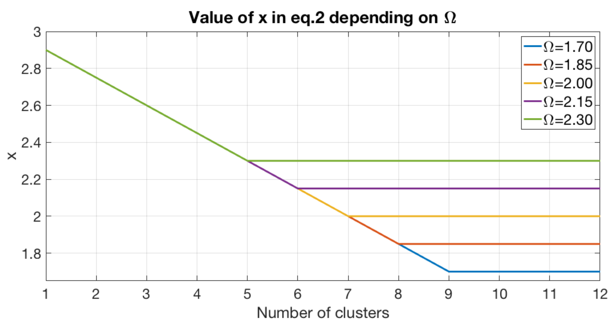
x is a parameter that must be tuned, and whose value must depend on the number of clusters. The lower
x, the more restrictive the condition to create a new node. Values of
x used in this work vs. number of clusters can be seen in
Figure 5. As shown in this figure, x is less restrictive for a low number of clusters, but it is necessary to limit it from a specific number of clusters. This limit is established depending a parameter (
) which has to be tuned (
Table S4).
x remains constant at {1.7, 1.85, 2, 2.15, 2.3} when
or
respectively.
At the end of the Node Level Loop Closure, all the nodes that satisfy Equation (
4) are considered candidate nodes and introduced in the set
. After that, the Image Level Loop Closure is activated to try to retrieve the specific image from these nodes that closes the loop. In some occasions, the Node Level Loop Closure may not find any candidate node that closes the loop. In that case, it outputs an empty set of nodes, and it is considered that the new image does not close the loop with any of the existing nodes so far.
4.2. Image Level Loop Closure. Position and Orientation Descriptors
This algorithm activates if the Node Level Loop Closure is successful and outputs a non-empty set
of candidate nodes. In this case, it is necessary to determine which specific image or images close the loop, being the most similar to
. Given the set of candidate nodes
, all their corresponding images
are evaluated to find the image
which is the most similar image to
. The problem is solved using two different similarity metrics, described in
Section 3. These similarity metrics are computed between the descriptor of the image
and every of the descriptors of the
candidate images. Using both metrics, the comparison combines position and orientation information.
First, position information is obtained comparing the position descriptor of the image
with the position descriptors of the images
using
Euclidean distance. Second, the orientation information is used. In this case the method estimates the relative shift between each candidate image
and
. Then the panoramic image
and its associated descriptor are shifted, in such a way that after this shift, both images have the same relative orientation. Then the distance between the orientation descriptors is calculated using
Euclidean distance (Equation (
5)), where
is the descriptor obtained from the new image
and
is the descriptor of each of the images
contained in the candidate nodes
after running the Node Level Loop Closure process.
This process is repeated for all the images
contained in the set of candidate nodes
. After that, the method calculates the inverse of these distance measures, so the images with small distances (images that are more similar) will have higher similarity measure. Then, the result is normalized in such a way that the sum of the similarities is equal to 1. Next, the position and orientation similarity measures are multiplied to obtain the final similarity measure that combines both kinds of information. The image
with the associated higher result is then retrieved by the Image Level Loop Closure (and its node as the most similar node to
. It is possible to see an example of these measures in
Figure 6, where
Figure 6a shows the similarity measures between the image
and the images in the candidate nodes when using position descriptors;
Figure 6b shows the same similarity comparison but using orientation descriptors and
Figure 6c shows the final similarity measures obtained by multiplying position and orientation measures. These results (final similarity measure) are the data used to retrieve both the image and the node that close the loop with
. Only the images
that belong to the candidate nodes
have a value in these figures, the other images are considered to have null measure.
If no node is selected as candidate node the Image Level Loop Closure process cannot be run. Therefore, the image is not assigned to any node, and it remains unclassified, waiting for information from the next images (those which are subsequently captured by the robot). When a set of consecutive images are left unclassified, a new node has to be created with them and the node representatives are recalculated (the node representative is the mean descriptor of the images contained in the node).
4.3. Prominence Condition
As explained in
Section 4.1, the Node Level Loop Closure process selects
possible nodes. Among them, the Image Level Loop Closure process finds the most similar image (
) which closes the loop. The node to which
belongs, is the finally selected node. Prior to selecting this node
, the image detected as the most similar to
should meet a prominence condition.
The prominence measures how much the peak of the similarity curve (
Figure 6c) stands out due to its intrinsic height and its location relative to other peaks. This condition is taken into account because not only a high peak should occur to close the loop, but also that peak should be very distinct compared to its neighbours. The image selected from the Image Level Loop Closure should fulfil the condition presented in Equation (
8). In this equation,
is the prominence value of the candidate image,
is the mean prominence of the candidate images contained in
.
is a threshold, which is empirically tuned from the experiments as
.
4.4. Centroid Condition
As detailed in the previous subsections, the node Level Loop Closure selects first
candidate nodes. Among them, the Image Level Loop Closure finds the most similar image which closes the loop and helps select the final node. In order for a selected node to be accepted as the final node, it must fulfil the condition of Equation (
9) below. This condition evaluates how the position of the node representative shifts when the new candidate image is added to the selected node. In the condition, the distance between the node representative before (
) and node representative after adding the descriptor of the new image (
) has to be lower or equal to the maximum influence on the node representative effected by the images already contained in the node.
where
denote all descriptors of the images contained in the node
.
The process presented in
Section 4.1,
Section 4.2,
Section 4.3 and
Section 4.4 is summarized in the pseudocode Algorithm 1. Starting from the current set of clusters in the map
= {}, their associated data (
, and for
) and the descriptors of each previous image
, it is possible to determine if a new image
, whose descriptor is
, has to be assigned to any previous node or not.
| Algorithm 1. Pseudocode for Node and Image Level Loop Closure, applying Prominence and Centroid Conditions. |
1: NodeLevelLoopClosure ()
2: = {} initial set of clusters
3: , mean descriptor and covariance matrix of cluster
4: for l=1 to number of clusters C do
5: (Equation (3))
6: if then (Equation (4))
7: ;
8: end if
9: end for
10: end NodeLevelLoopClosure
11: ImageLevelLoopClosure (, ,)
12: for k= 1 to images in do
13: (Equation (5));
14: find the most similar image using Equation (7);
15: if meets then (Equation (8), Prominence Condition)
16: if meets then (Equation (9) Centroid Condition)
17: and its node close the loop;
18: is included in ;
19: , and are updated;
20: else
21: does not meet Equation (9);
22: is not included in ;
23: end if
24: else
25: does not meet Equation (8);
26: is not included in ;
27: end if
28: end for
29: if then
30: is not assigned to any node;
31: The existing nodes are not updated and will be evaluated in subsequent steps;
32: end if
33: end ImageLevelLoopClosure |
4.5. New Node Creation
The methods presented so far detect the node to which the new image
belongs. However, as explained before, the new image may not be assigned to any previous node. That may occur either because the new image is quite different to the existing node representatives or because it does not fulfill either the prominence condition (
Section 4.3) or the centroid condition (
Section 4.4).
Once a considerable number of images consecutively captured are considered not to belong to any cluster, a new cluster is created. The new cluster is modelled with its mean descriptor and covariance matrix . In order to obtain a new cluster which is significantly different to the ones already existing in the map, the average distance between the representative of the new node and the representative of the other nodes (using Euclidean distance) has to be higher or equal to the average distance among the representatives that already exist. If the new cluster does not fulfill this condition, this new cluster cannot be elected in further Node Level Loop Closure processes. In this way, new images continue to be evaluated without considering this cluster but if they are still not assigned to any node but they are similar enough to the cluster , they are included to that cluster until the distances from the representative of to other representatives is higher or equal to the average distance among the representatives of the other clusters in the map. This condition tries to guarantee that clusters are different enough among them and that they do not spread excessively along the space of features.
4.6. Node Merging
According to the previous processes, the number of clusters constantly increases. Therefore the resulting number of clusters is sometimes higher than necessary and images that represent adjacent and/or visually similar zones may be included in a unique cluster. The proposed method has the possibility to decrease the number of clusters by merging similar nodes when necessary. That is possible because the method detects when two clusters are similar and the map would be more consistent if they are merged. A new condition is introduced and a newly created node
has to exceed a specific dissimilarity threshold to the other clusters. If an existing cluster and a new one are similar, they are merged in a unique cluster. To solve this problem the Mahalanobis distance is used as in Node Level Loop Closure process. Equation (
10) shows this condition in the node merging process
where l = 1,2,…,
C and
C is the number of clusters before creating
. To detect if the node
should merge with another node
,
is evaluated. This distance has to satisfy the condition of similarity presented in Equation (
11), where
and
are the mean and the standard deviation of the Gaussian distribution calculated with the data of node
, calculated as detailed in
Section 4.1.
y is a parameter which has to be empirically tuned (
Table S4). The higher it is, the less restrictive the condition is, so the algorithm is more prone to merge similar clusters. Experiments show that this threshold should take a value between 1 and 2. If
the condition is very restrictive so less mergers are done and more clusters will be in the final map, but when
the condition is less restrictive, so more mergers are done and less clusters will be at the end. Experiments to test the values of
y are carried out in
Section 6.
5. Image Sets for Experiments
The proposed algorithms are tested with several sets of images captured under real operating conditions. The datasets used are the INNOVA dataset [
22] captured by ourselves and the COLD database [
53], a third party publicly available dataset which provides robot trajectories in some buildings of the Freiburg and Saarbrücken universities. These three trajectories provide a good choice to perform hierarchical incremental mapping because they represent real environments that experience the typical phenomena that can occur during real operation such as noise, occlusions of the images, changing lighting conditions, movement of people or even some objects or pieces of furniture etc. For that reason these sets of images constitute a challenging scenario to test the robustness of the incremental mapping algorithms.
The different image sequences are recorded by a mobile robot, which is equipped with an omnidirectional camera. The catadioptric vision system is made using a hyperbolic mirror mounted in front of the camera on a portable bracket. The program receives the omnidirectional images and it transforms them into panoramic ones and starts the mapping process, updating the map every time that a new image
arrives according to
Section 4. Additionally, the robot is equipped with wheel encoders and a laser range scan, which are used to obtain the ground truth, for comparative purposes. However, the proposed method does not use these data and it carries out the incremental mapping with pure visual information.
Figure 7 shows the robot and the camera used to capture the INNOVA dataset. Complete information about the equipment used to capture the COLD dataset can be found in reference [
53].
Figure 8 shows some sample images from all the datasets.
Table 1 shows some specifications about the 3 trajectories and the number of images taken in each trajectory. Each route contains some loops so they permit testing the Node Level and Image Level Loop Closure processes. Finally, we consider essential to say that these environments are a challenging choice because across the route many walls are made of glass and there are lots of windows so the outdoor weather and lighting conditions could have a negative impact upon the mapping task.
6. Experiments
In this section, the methods proposed for hierarchical incremental map creation are tested using the image sets introduced in the previous section. Firstly some images are taken to create the first cluster in a supervised method. Once the first cluster is created, the process can start in order to create new clusters, incrementally updating the map every time a new image arrives.
6.1. Parameters to Describe the Images
As explained in
Section 3, using global-appearance descriptors, each panoramic image is reduced to a vector
whose size depends on the parameters used in this description process. These parameters are outlined in
Table S2. In this work, we use
with the HOG position descriptor. In this case, the position vector size is
. For the orientation descriptor
,
and
, so the panoramic image is reduced to a vector whose size is
. In the case of gist, the parameters were kept constant in
and
for the position descriptor. Using these parameters the descriptor size is
. In the case of the gist orientation descriptor, it is calculated with
,
,
and
and each image is transformed to a vector
.
6.2. Parameters to Perform the Loop Closure Processes
When a new image arrives, the first step is to know if it belongs to an existing cluster. As detailed in
Section 4, to perform the Node Level Loop Closure, the
Mahalanobis distance is used, (Equation (
3)). After that, it is possible to detect if the image descriptor
may belong to a specific node
, storing all the candidate solutions in the set
.
Once the candidate nodes are selected, their images are compared with
using
Euclidean distance, Equation (
5), where
are all the candidate descriptors from the Node Level Loop Closure. The Image Level Loop Closure detects the most similar image among them, named
. After detecting
, the image has to fulfill the Prominence and Centroid Conditions (
Section 4.3 and
Section 4.4). Furthermore, the process evaluates if two nodes are similar enough to be merged (
Section 4.6).
As described in
Section 4, these equations depend on different parameters that have an influence on the results. Equation (
4) depends on
x. It establishes how restrictive the process is to close the loop in the node level. The lower
x is, the easier to close the loop.
x must depend on the number of clusters (C) and it is tuned as
; with limits depending on
,
Figure 5 shows graphically these values. Another parameter is
y, which is used in Equation (
11) and it influences the node merging; the lower
y, the easier to merge similar nodes. Finally, the parameter
appears in Equation (
8). Once
is retrieved, this equation evaluates the prominence of the result to ensure that the retrieved image has a peak on the similarity curve higher enough compared to its the neighbours. The higher
is, the more prominent the peak must be. During the experiments
is constant,
. These parameters are summarized in
Table S4.
6.3. Evaluation
The relative performance of a clustering framework can be evaluated by means of the silhouette. Silhouette evaluates the compactness of each cluster, i.e., the degree of similarity between each descriptor and the other descriptors of the same cluster, comparing it with the descriptors that belong to the other clusters. The average silhouette (
S) of all the entities (images descriptors) is calculated with Equation (
12). The higher S is, the more similar each descriptor is to the descriptors in its own cluster and the more different to the descriptors in the other clusters. The maximum value of the silhouette is 1, indicating that the resulting clusters contain well-separated images; the descriptors in each cluster are very similar among them and different to descriptors in the other clusters. By contrast, the minimum value is −1, which means that the resulting clusters do not separate correctly the information. In this work, the silhouette is used to evaluate the compactness of the clusters. Therefore, instead of using the similarity in the feature space, world coordinates are used.
In Equation (
12),
C is number of clusters and
the average silhouette of the descriptors contained in the cluster i. The silhouette of each descriptor
is calculated using Equation (
13).
where
is the average distance between the capture point of
and the capture points of the other descriptors in the same cluster and
is the average distance between the capture point of
and the capture points of the other descriptors in the different clusters. The information about the capture points is known because the ground truth of the data set is available, so this information is used to quantify the performance of the mapping algorithm. Notwithstanding, it is worth highlighting that the mapping task is carried out with pure visual information.
In addition, the number of clusters obtained after the process will also be shown in order to evaluate how the parameters have an influence upon this number.
6.4. Results
6.4.1. Influence of the Parameters on the Performance of the Algorithm
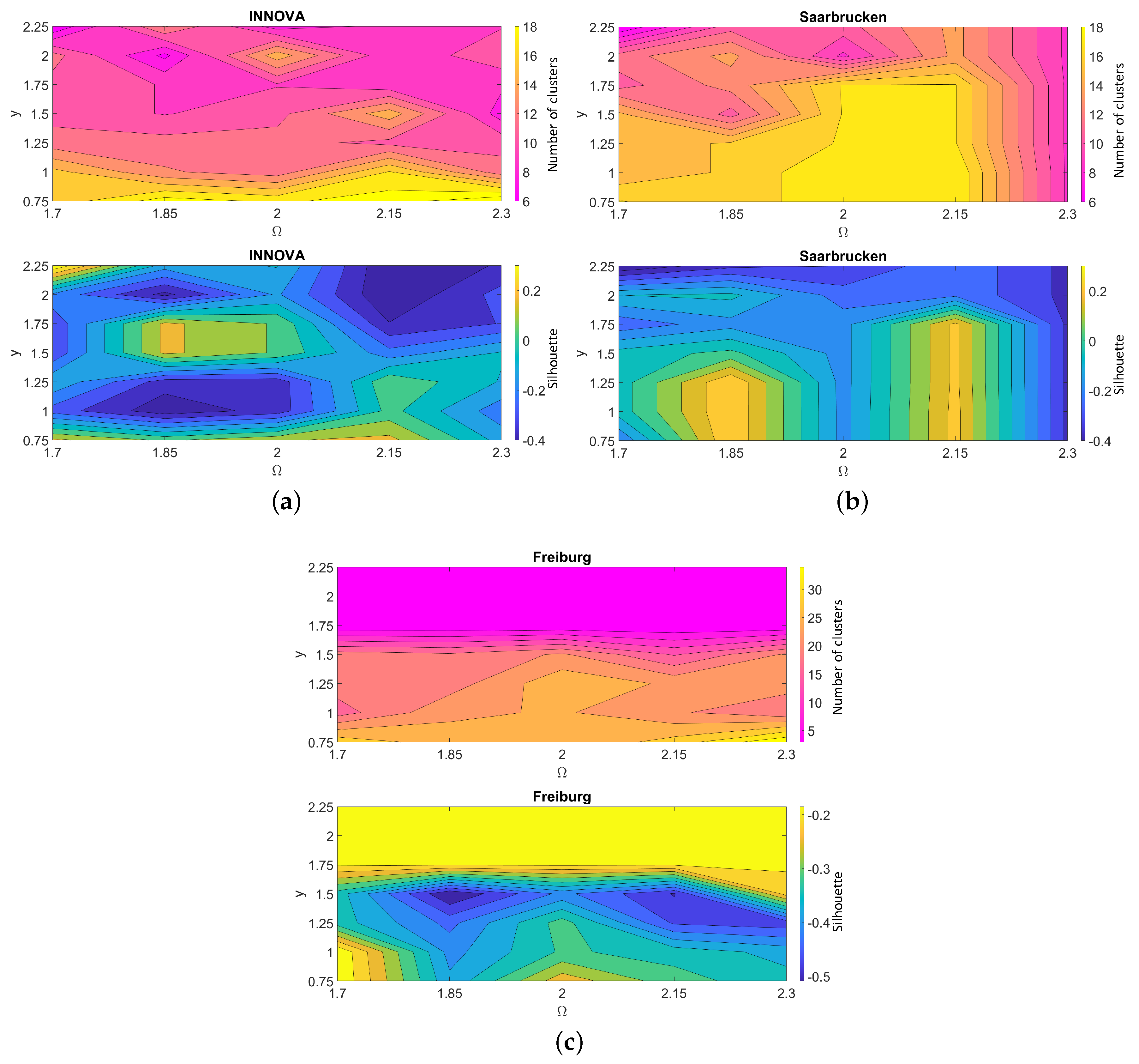
Figure 9 shows the results obtained with the HOG descriptor, and
Figure 10 with gist for (a) INNOVA, (b) Saarbrücken and (c) Freiburg datasets. In both figures, the first row shows the number of clusters obtained once all the images of each trajectory were processed by the proposed algorithm. The second row presents the average silhouette of the descriptors. These figures show the influence of the parameters
y and
, which are introduced in
Table S4.
First, considering parameter
y, as expected, the higher
y is the fewer clusters will be in the final map. The effect of this parameter is less significant when gist is used, as shown
Figure 10. Second,
limits
x, the parameter used in Equation (
4). If this value is low, more nodes can be selected on the Node Level Loop closure so it can be more difficult to obtain a high number of consecutive images without being in a cluster so the effect of creating new nodes decreases. However, if this value is too high it may lead to some images in a row not being assigned to any node when no new cluster should be created in the Node Level Loop Closure process. As
Figure 9 and
Figure 10 show, when HOG is used, the parameter
y has more influence on the number of clusters than
does, yet with the gist descriptor, the latter has greater influence.
The second row of each subfigure in
Figure 9 and
Figure 10 shows the average silhouette after the mapping process. In general, medium values of
offer a higher silhouette but the effect of
y is more variable. To better study the results,
Table 2 shows the maximum values of silhouette and the number of clusters obtained with the different datasets. It also shows the values of the parameters that lead to that maximum silhouette. It shows how values of
around 1.85 offer the best results although when using gist descriptor good silhouettes can be also obtained with higher
values. Meanwhile, the results are not substantially dependent on
y. As it is possible to observe, better results are obtained using the HOG descriptor. This behaviour was observed among different experiments and situations, which makes us conclude that HOG is a more suitable option to describe the images with the objective of creating a map incrementally. In addition, the silhouette obtained with the Freiburg dataset is substantially lower than the silhouette obtained with the two other datasets. The reason can be twofold. On the one hand, the route contains a large number of images, and it has some spaces which are visually similar, which challenges the mapping algorithm. On the other hand, the Freiburg environment contains several glass walls, and large and numerous windows, which produce saturations in the images and mixing between the information of adjacent rooms. These phenomena also have a negative impact upon the performance of the method.
6.4.2. Batch Spectral Clustering Results
For comparative purposes, we consider a batch spectral clustering algorithm [
11] as benchmark. It is worth highlighting that this batch spectral clustering algorithm has complete information about all the descriptors from the beginning of the process, and can calculate all the mutual similitudes to perform the clustering process. Therefore, it constitutes a powerful benchmark to compare the relative performance of our proposal. To use this batch technique, the number of clusters has to be set initially and all the images must be available, for this reason it is not a good option to create maps incrementally, as the robot explores new areas.
Figure 11 and
Figure 12 show the results after using a batch spectral clustering method and either HOG or gist descriptors respectively. These figures represent average silhouette versus number of clusters.
Figure 11 shows the average silhouette when the HOG descriptor is used. This figure shows that the average silhouette decreases when the number of clusters continuously increases. The results obtained with the INNOVA dataset show that the silhouette is between 0.1 and 0.3; in particular if we observe the result with 6 clusters (which lead to the maximum silhouette with the proposed method) silhouette is 0.13 while with the proposed method is 0.3973. In the case of the Saarbrücken dataset, while the silhouette obtained with batch spectral clustering is between 0.1 and 0.3, the results with proposed incremental method are between −0.4 and 0.3. Observing the result with 16 clusters (which led to the best silhouette with the proposed method) we note this is about 0.15 as opposed to 0.2756 with the proposed algorithm. Finally, regarding the Freiburg dataset, while the results using batch spectral clustering are between 0.1 and 0.25, results using the incremental method are among −0.5 and −0.15. The maximum value of silhouette of the proposed method is equal to −0.1526 with 30 clusters, while the batch clustering method provides a silhouette of 0.13 with the same number of clusters.
Additionally,
Figure 12 show the silhouette when the gist descriptor is used. In this case, the results are less similar to the results obtained with the proposed method. Again, the higher the number of clusters is, the lower the silhouette values are. The best silhouette obtained with gist and the INNOVA dataset is 0.2556 with 6 nodes, the batch clustering method leads to a silhouette equal to 0.38 with the same number of nodes. With the Saarbrücken dataset, silhouette results with a high number of clusters are around 0.25 and 0.4 with the batch method and 0.1262 (19 clusters) with the proposed method. Finally, the results output by the batch clustering method on Freiburg show a silhouette between 0.1 and 0.25 but using the proposed incremental clustering process the maximum silhouette is −0.1449, obtained with 34 clusters. With 34 clusters the silhouette obtained with batch clustering is 0.15. The results of this comparative evaluation between the proposed method and the benchmark algorithm are summarized in
Table 3. This table includes the maximum silhouette obtained with the proposed method, and the silhouette obtained with the batch spectral clustering with the same number of clusters. It is necessary to highlight the fact that the proposed method provides better results with HOG in the Innova and Saarbrücken datasets. It is especially relevant, considering that the proposed method permits building the map as the robot explores the environment (i.e., it works with incomplete visual information) but the batch clustering needs to have all the images captured before running the algorithm. The results with the Freiburg dataset are less conclusive, due to the features of this dataset, commented previously. HOG stands out again as an efficient image description method with incremental mapping purposes.
6.4.3. Bird’s Eye View of the Capture Points
Figure 13,
Figure 14 and
Figure 15 show a bird’s eye view of the capture points of the three datasets in different points of the proposed incremental clustering process. These capture points are shown with different shapes and colors, depending on the cluster they belong to.
Figure 13j,
Figure 14g and
Figure 15j show the result after completing all the proposed incremental mapping method, and the subfigures show how the clusters are being created while the map is updated. Observing the pairs of subfigures:
Figure 13c,d,f,g or
Figure 15e,f it is possible to see how node merging (
Section 4.6) works. Initially, there are several clusters and after including some new images and creating new clusters or making a specific cluster larger, it is possible to obtain similar clusters, so the merging process is launched and it results in a lower number of clusters. Finally,
Figure 14b,e shows how transition between rooms resulted in an increased number of clusters. After 399 images, the process has detected 7 clusters but from moment
Figure 14e to the end of the process the robot has moved across a long corridor and only changes the room once, for that reason only 2 clusters are created on that process. Others characteristics such as loop closure can be observed in the figures.
7. Conclusions
This work presented a method to create hierarchical topological maps incrementally, updating the map every time a new image arrives. The framework is based on the development of an incremental clustering algorithm, presented throughout the paper. The experiments were made in real indoor environments where the robot navigates under real operation conditions, including illumination variations and changes introduced by human activity. The robot is equipped with an omnidirectional vision system, and the only information used to build the hierarchical map are the images captured by this system. To describe the images two different global-appearance methods were considered: HOG and gist. The experimental section showed the performance of the proposed algorithm and the effect of the most relevant parameters on the final result. Also, a comparative evaluation with a batch spectral clustering algorithm is performed.
The relative accuracy of the method is studied by means of the average silhouette, calculated considering as entities the capture points of every image (ground truth). First, HOG proved to output better results, such that the average silhouette obtained with the proposed incremental method is similar to the silhouette output by the batch spectral clustering method despite the fact that the proposed algorithm only has partial information at each step. In fact, if the parameters are tuned properly if can offer better results than the batch spectral clustering. The results show that in the case of HOG, it is especially important tuning correctly the parameter y, as it has a strong influence on the final number of clusters. Also, the performance of the proposed algorithm degrades when the dataset contains an excessively high number of images, presents complex features (i.e., numerous windows or glass walls) or is prone to visual aliasing.
The results might be considered successful since our incremental algorithm starts with a reduced number of images and updates the map (clusters) every time a new image arrives whereas the batch clustering algorithm has complete information on all the descriptors from the beginning of the process, and can calculate all the mutual similitudes to perform the clustering process. Additionally, gist proved to perform less robustly and the silhouettes obtained with batch spectral clustering are relatively higher. Therefore, the proposed incremental method along with omnidirectional images and the HOG descriptor constitutes the most suitable option to perform incremental mapping.
This work opens the door to new research works on incremental hierarchical map creation using global-appearance description methods in mobile robotics. Once we have tested the robustness and efficiency of the methods in real environments including human activity and presence of changes in the position of some objects, the next step is to improve the algorithm and adapt it to be used in large and outdoor environments. In this sense, we will focus in particular on the problem of abrupt changes of the lighting conditions and changes across seasons, as it is one of the issues that may have a more negative impact upon the visual mapping algorithms.


