Finite-Time Path Following Control of an Underactuated Marine Surface Vessel with Input and Output Constraints

Abstract
1. Introduction
- (1)
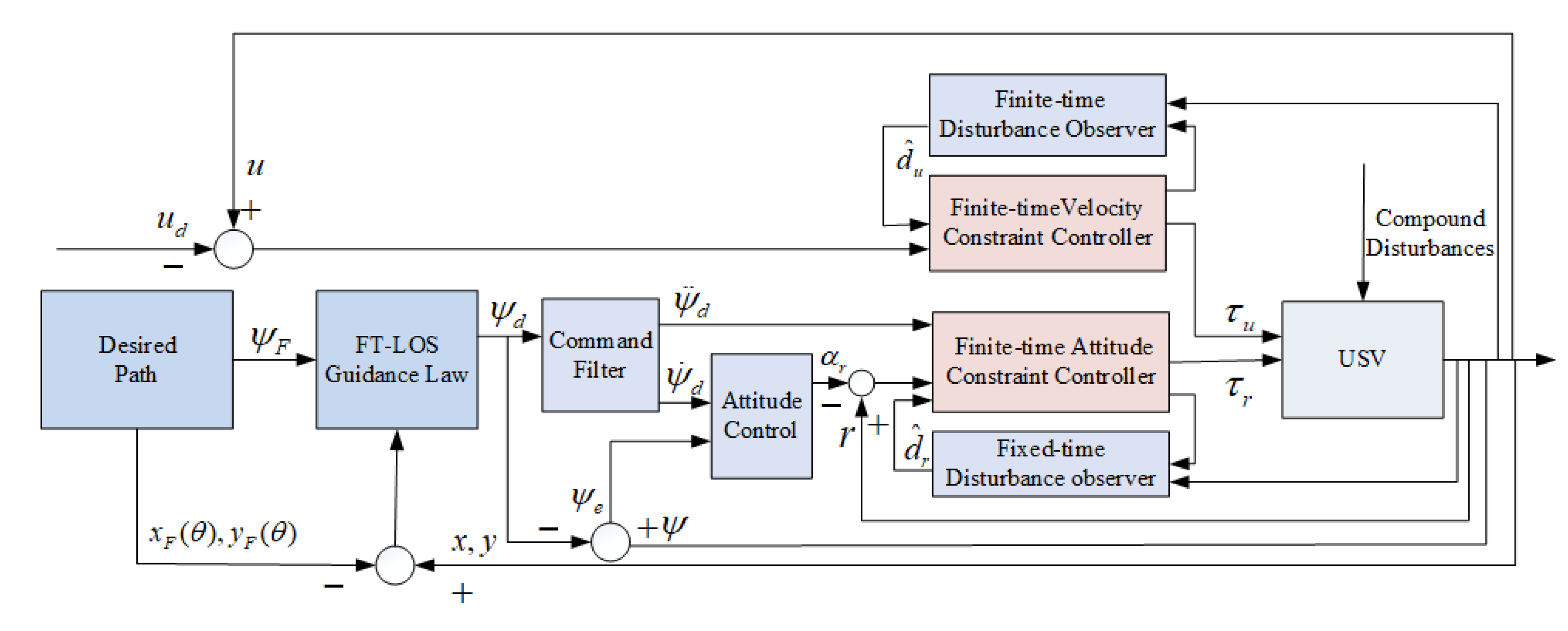
- A finite-time line-of-sight (FT-LOS) guidance law is designed by integrating a time-varying BLF into the classical LOS guidance law design process. The proposed FT-LOS guidance law can ensure that the position errors will not exceed the error constraints, and converge into a small neighborhood around zero in finite time.
- (2)
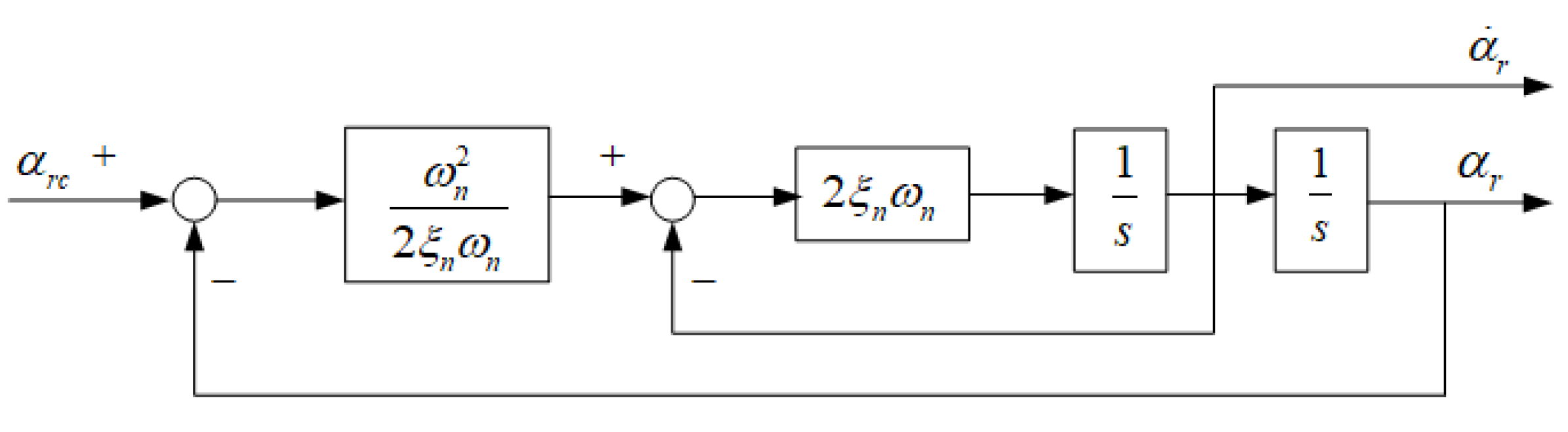
- The finite-time attitude constraint controller and the finite-time velocity constraint controller are designed to achieve tracking control in finite time. A command filter is designed to eliminate the complex calculation of the virtual control law.
- (3)
- The finite-time disturbance observers are proposed to reduce the compound disturbance. In addition the finite-time input saturation compensators are designed to avoid the actuator saturation and satisfy the finite-time convergence requirement.
- (4)
- The stability analysis shows that the proposed finite-time path following control algorithm can strictly guarantee the constraint requirement of the position, and all error signals of the whole closed-loop control system can converge into a small neighborhood around zero in finite time. Comparative simulation results illustrate the effectiveness and superiority of the proposed finite-time control scheme.
2. Preliminaries and Problem Formulation
2.1. Preliminaries
- (i)
- Finite-time convergence: For every , is defined on , for all , and .
- (ii)
- Lyapunov stability: For every open neighborhood of 0 there exists an open subset of N containing 0 such that, for every , for all .
2.2. Model of Underactuated Marine Surface Vessel
- (1).
- The heave, pitch and roll motions are neglected in path following on the horizontal plane.
- (2).
- The vehicle is rigid body and its mass distribution is homogeneous, and the vehicle is port/starboard symmetric.
- (3).
- The origin of body-fixed is located at the center of gravity of the vehicle.
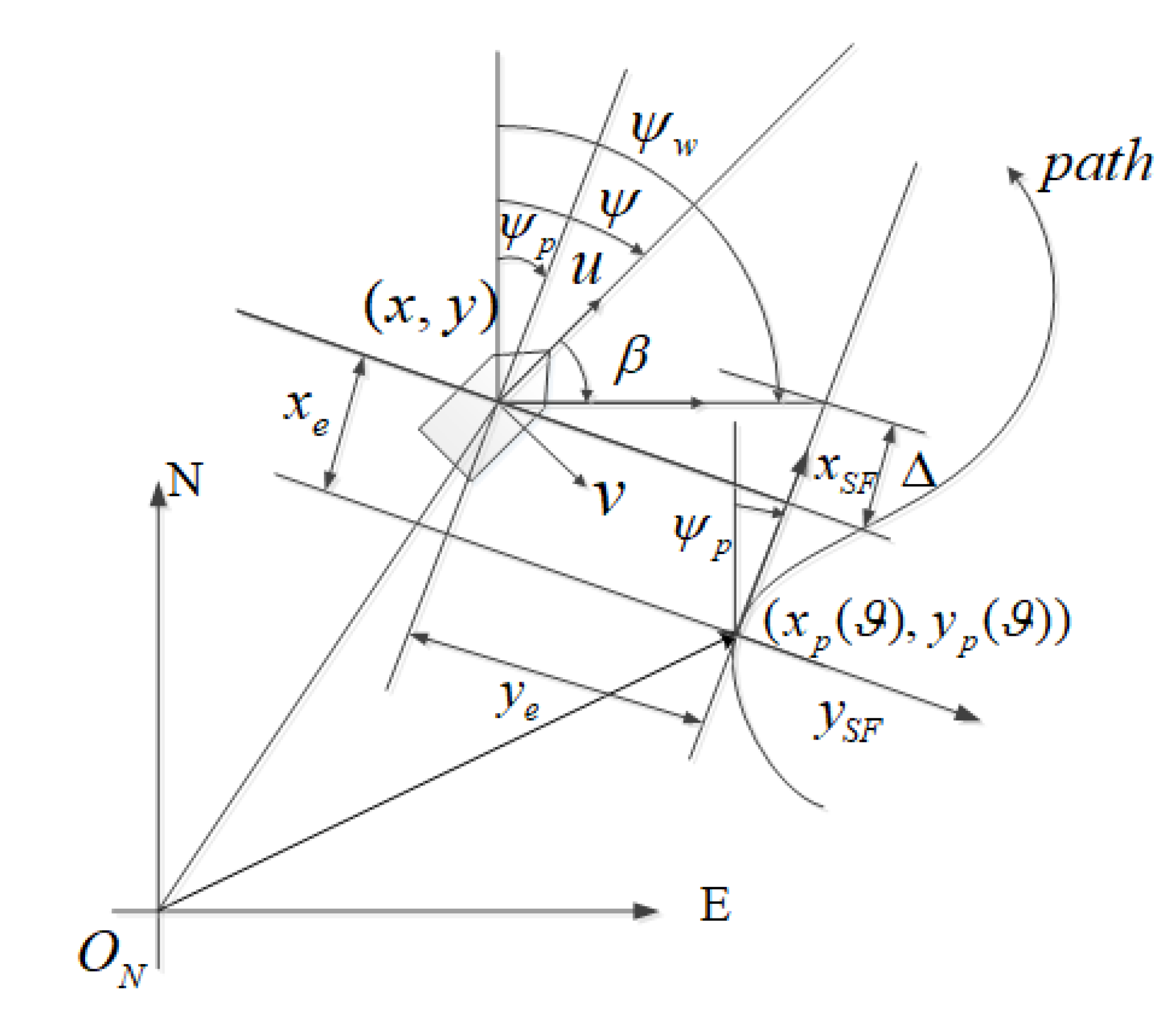
2.3. Path Following Error Dynamic
3. Finite-Time Path Following Control Algorithm Design
3.1. Ft-Los Guidance Law Design
3.2. The Finite-Time Attitude Constraint Controller Design
3.3. The Finite-Time Velocity Constraint Controller Design
4. Stability Analysis
- (i)
- All the error signals of the whole control system are uniformly ultimately bounded. Additionally, position errors meet the constraint requirements, that is and .
- (ii)
- The tracking error of an underactuated MSV can converge into a small neighborhood around zero in finite time.
- (i)
- According to (77), we have
- (ii)
- When , , where . Therefore, from (77), we can see:
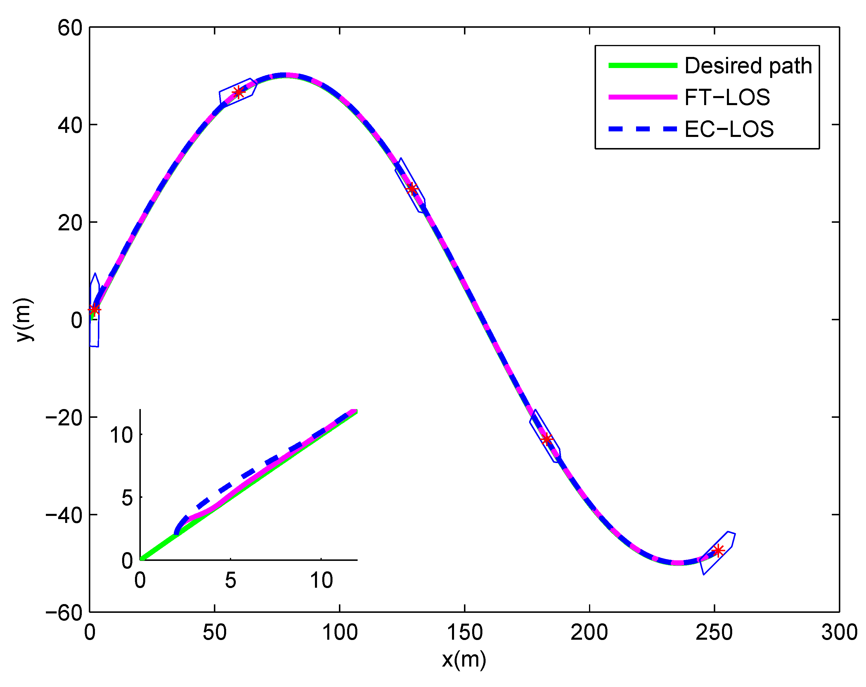
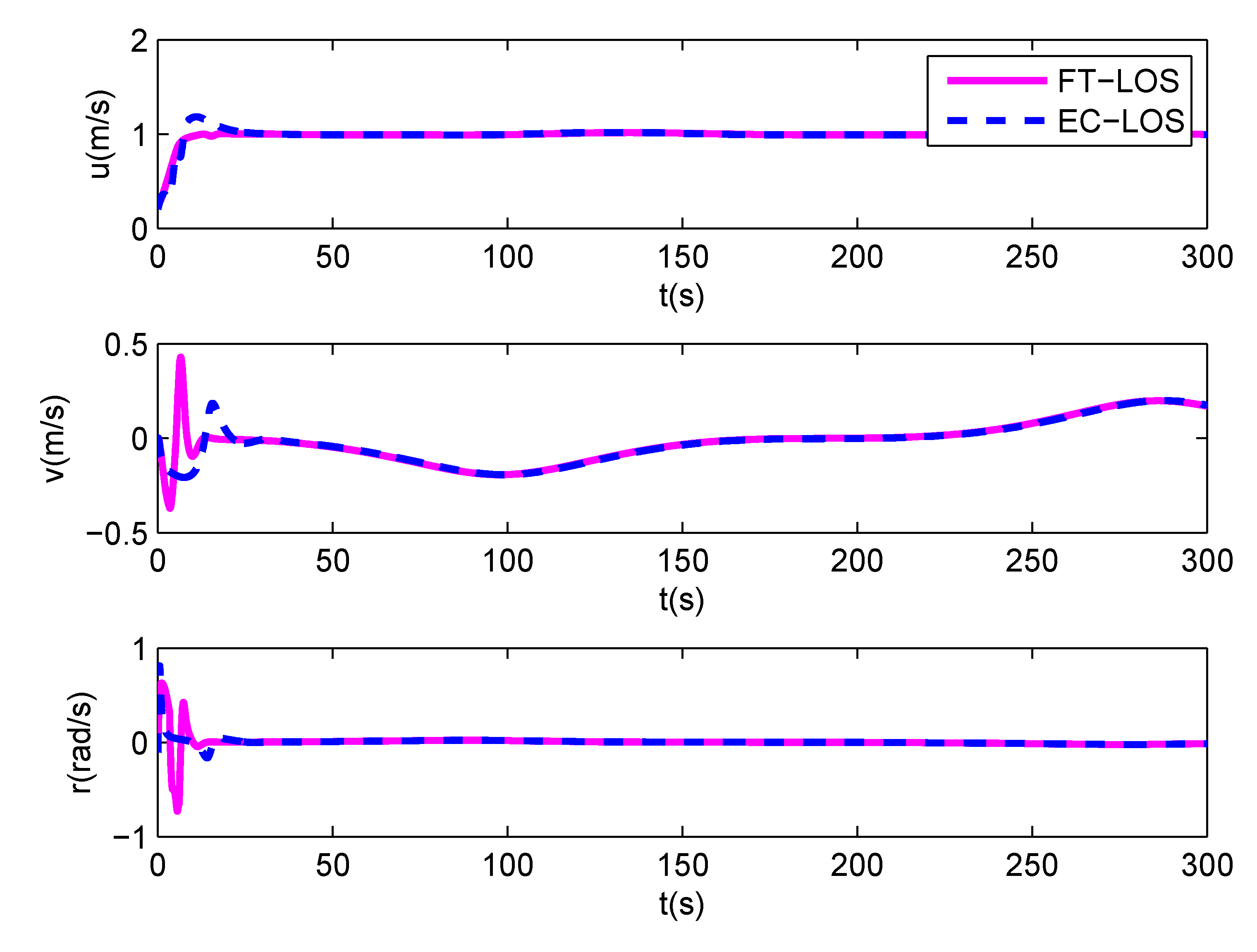
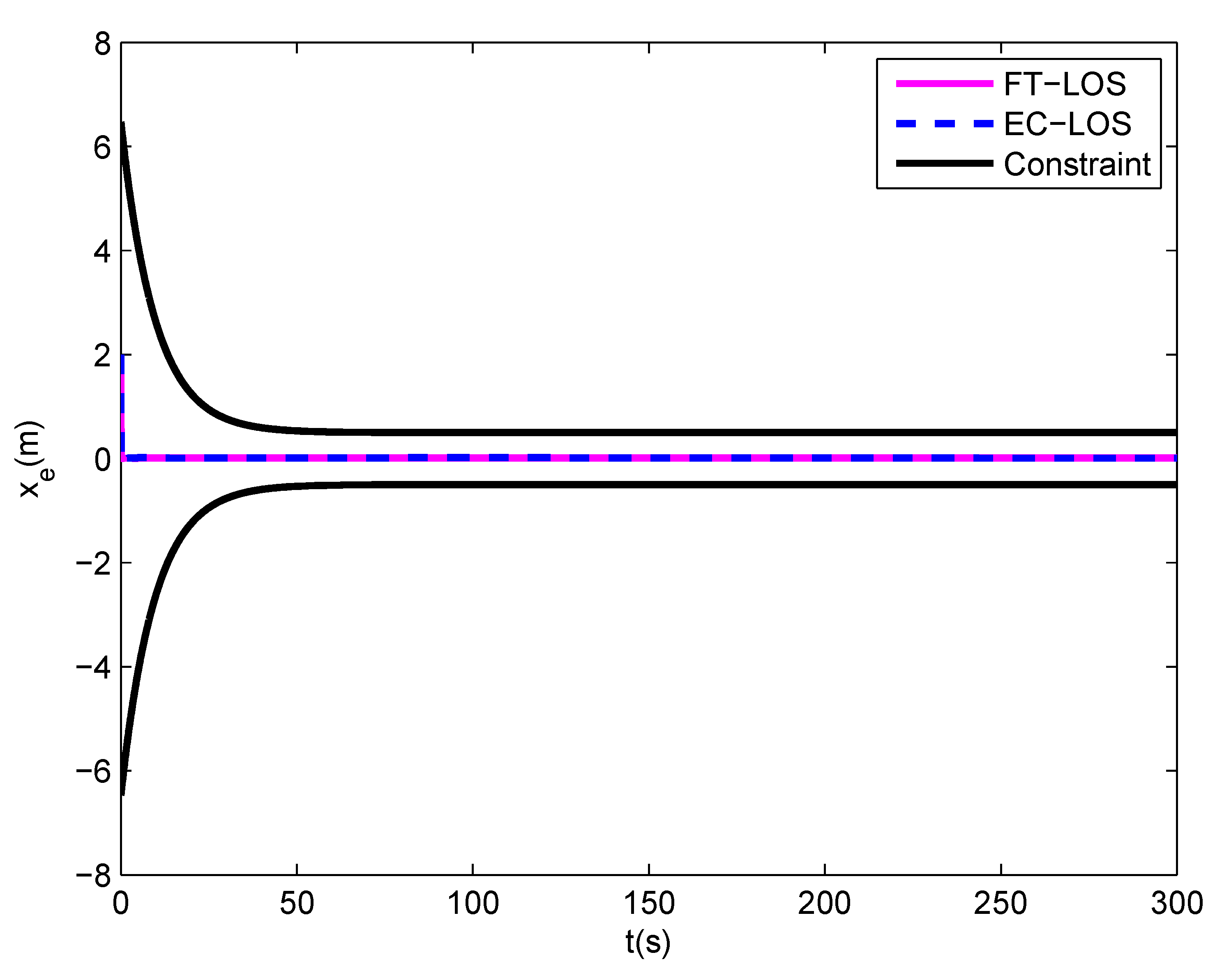
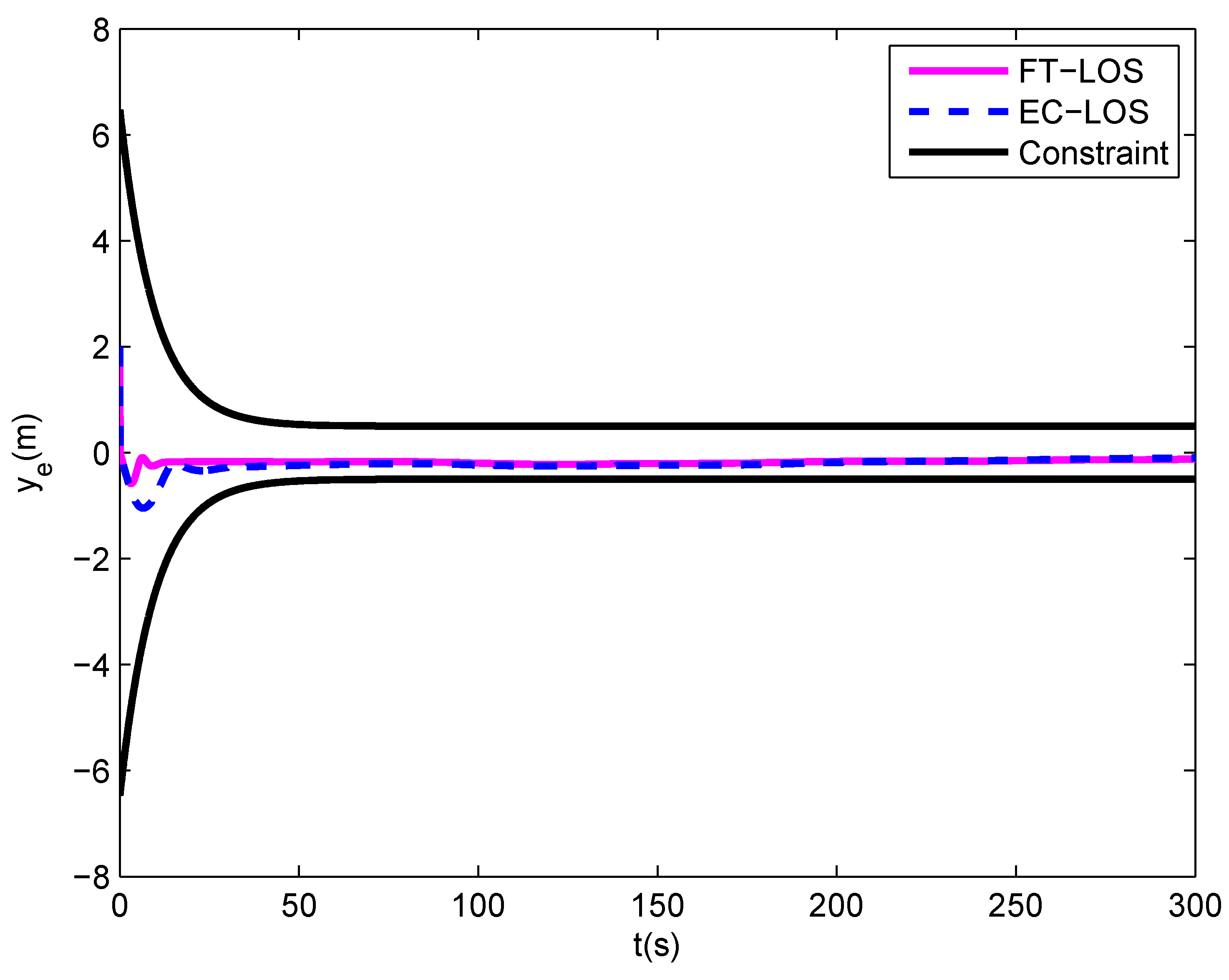
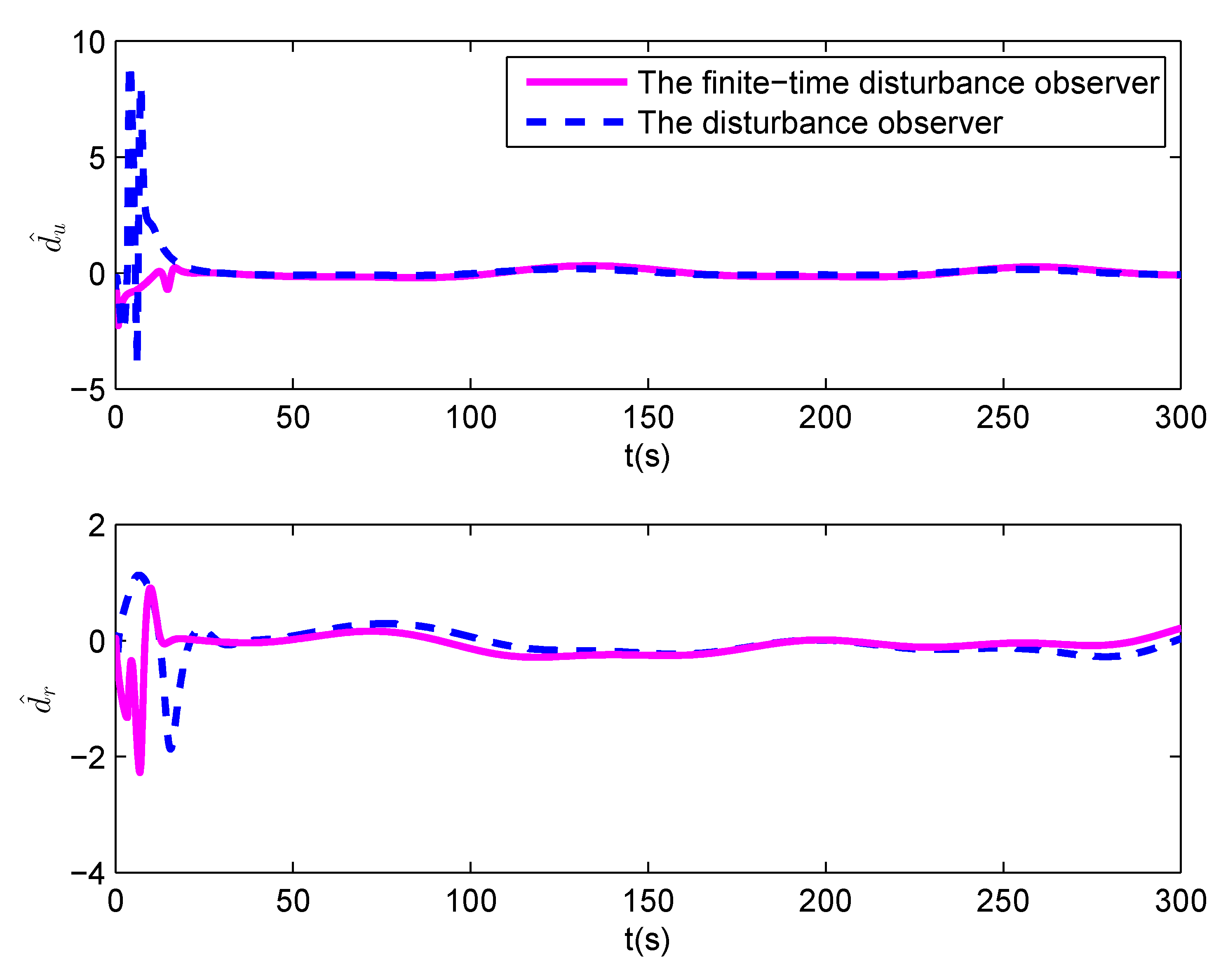
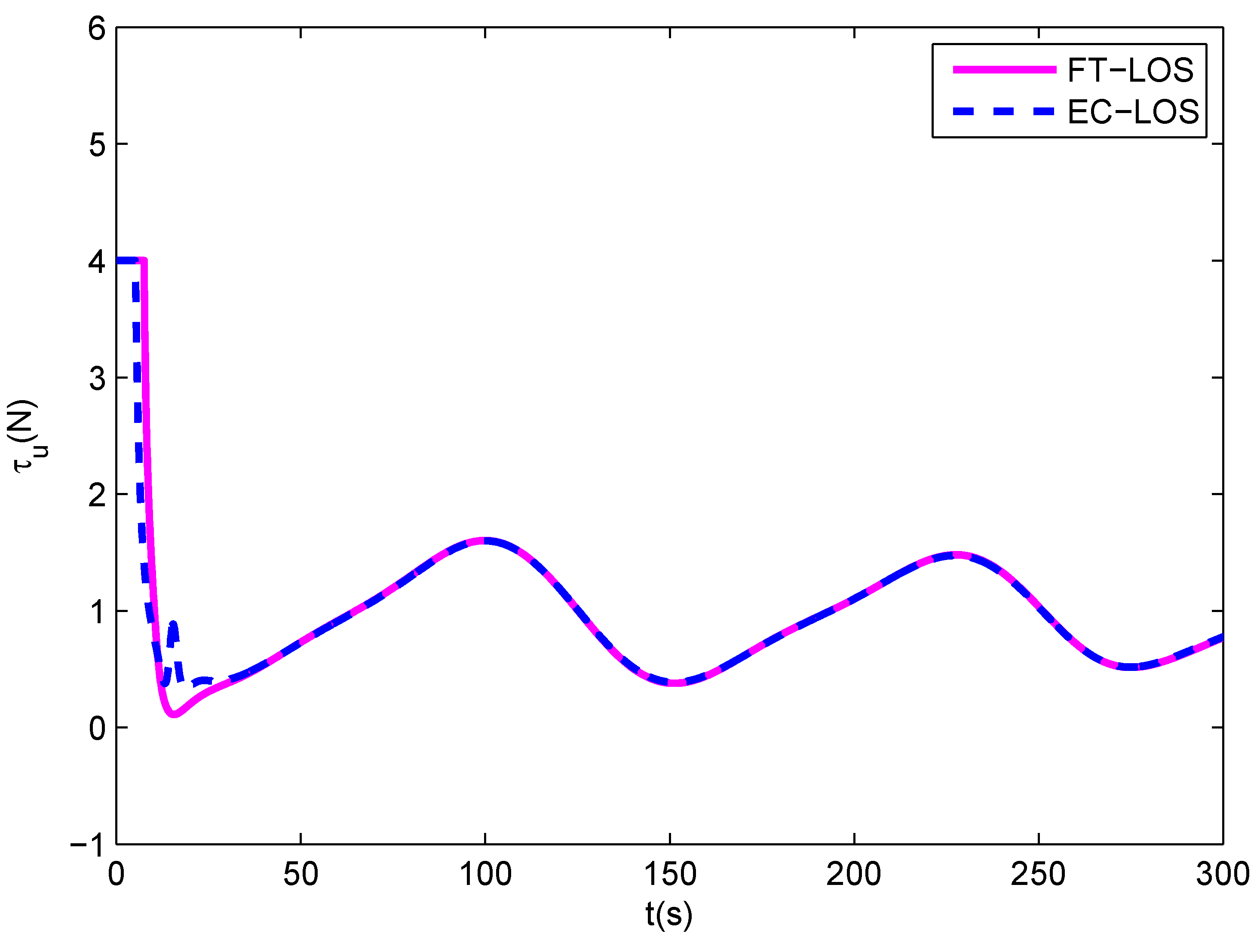
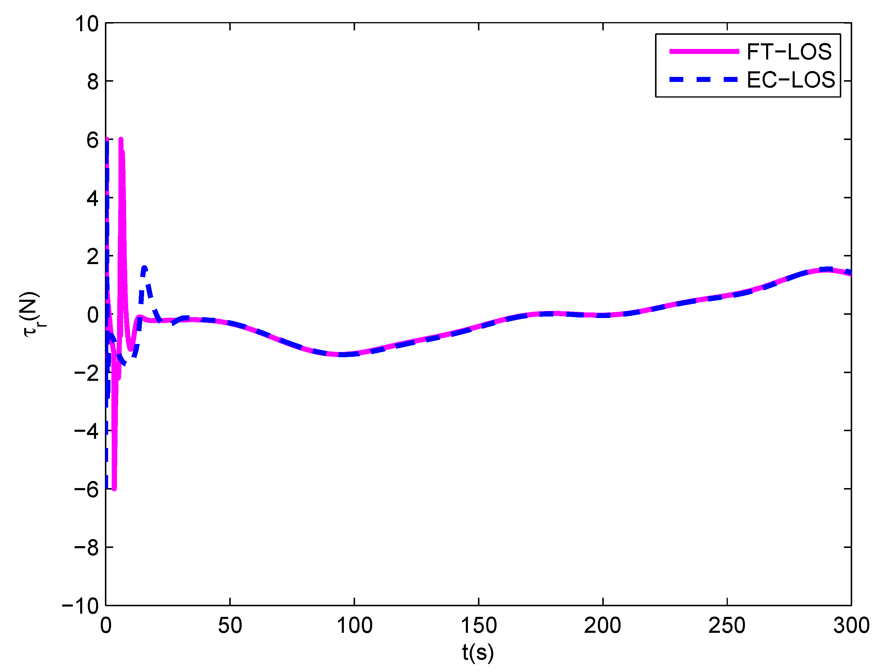
5. Simulation
6. Conclusions
Author Contributions
Funding
Conflicts of Interest
Abbreviations
| MSV | Marine surface vessel |
| LOS | Line-of-sight |
| BLF | Barrier Lyapunov function |
| FT-LOS | Finite-time line-of-sight |
| PLOS | Proportional line-of-sight |
| ILOS | Integral line-of-sight |
| EC-LOS | Error-constrained line-of-sight |
References
- Børhaug, E.; Pavlov, A.; Pettersen, K.Y. Straight line path following for formations of underactuated underwater vehicles. In Proceedings of the 46th IEEE Conference on Decision and Control, New Orleans, LA, USA, 12–14 December 2007; pp. 2905–2912. [Google Scholar]
- Breivik, M.; Fossen, T.I. Guidance Laws for Autonomous Underwater Vehicles; In Tech: Vienna, Austria, 2009; pp. 51–76. [Google Scholar]
- Breivik, M.; Hovstein, V.E.; Fossen, T.I. Straight-line target tracking for unmanned surface vehicles. Model. Ident. Control 2009, 29, 131–149. [Google Scholar] [CrossRef]
- Muresan, M.P.; Giosan, I.; Nedevschi, S. Stabilization and validation of 3D object position using multimodal sensor fusion and semantic segmentation. Sensors 2020, 20, 1110. [Google Scholar] [CrossRef] [PubMed]
- Fossen, T.I. Handbook of Marine Craft Hydrodynamics and Motion Control; Wiley: New York, NY, USA, 2011. [Google Scholar]
- Breivik, M.; Fossen, T.I. Path following for marine surface vessels. In Proceedings of the Oceans MTS/IEEE Technology-Ocean, Kobe, Japan, 9–12 November 2004; Volume 4, pp. 2282–2289. [Google Scholar]
- Børhaug, E.; Pavlov, A.; Panteley, E.; Pettersen, K.Y. Straight line path following for formations of underactuated marine surface vessels. IEEE Trans. Contr. Syst. Technol. 2011, 19, 493–506. [Google Scholar] [CrossRef]
- Balch, T.; Arkin, R.C. Behavior-based formation control for multirobot teams. IEEE Trans. Robot. Autom. 1998, 14, 926–939. [Google Scholar] [CrossRef]
- Fossen, T.I. Marine Control System: Guidance, Navigation and Control of Ship; Rigs and Underwater Vehicles: Trondheim, Norway, 2002. [Google Scholar]
- Fossen, T.I.; Breivik, M.; Skjetne, R. Line-of-sight path following of underactuated marine craft. IFAC Proc. (MCMC) 2003, 36, 211–216. [Google Scholar] [CrossRef]
- Børhaug, E.; Pavlov, A.; Pettersen, K.Y. Integral LOS control for path following of underactuated marine surface vessels in the presence of constant ocean currents. In Proceedings of the 47th IEEE Conference on Decision and Control, Caucun, Mexico, 9–11 December 2008; pp. 4984–4991. [Google Scholar]
- Caharija, W.; Pettersen, K.Y.; Bibuli, M.; Calado, P.; Zereik, E.; Braga, J.; Bruzzone, G. Integral line-of-sight guidance and control of underactuated marine vehicles: Theory, simulations, and experiments. IEEE Trans. Control Syst. Technol. 2016, 24, 1623–1642. [Google Scholar] [CrossRef]
- Fu, M.; Wang, T.; Wang, C. Barrier Lyapunov function-based adaptive control of an uncertain hovercraft with position and velocity constraints. Math. Probl. Eng. 2019, 2019, 1940784. [Google Scholar] [CrossRef]
- Zheng, Z.; Sun, L.; Xie, L. Error-constrained LOS path following of a surface vessel with actuator saturation and faults. IEEE Trans. Syst. Man Cybern. Syst. 2018, 48, 1794–1805. [Google Scholar] [CrossRef]
- Zheng, Z.; Huang, Y.; Xie, L.; Zhu, B. Adaptive trajectory tracking control of a fully actuated surface vessel with asymmetrically constrained input and output. IEEE Trans. Control Syst. Technol. 2018, 26, 1851–1859. [Google Scholar] [CrossRef]
- Zheng, Z.; Feroskhan, M. Path following of a surface vessel with prescribed performance in the presence of input saturation and external disturbances. IEEE/ASME Trans. Mechatron. 2017, 22, 2564–2575. [Google Scholar] [CrossRef]
- Nie, J.; Lin, X. Robust nonlinear path following control of underactuated MSV with time-varying sideslip compensation in the presence of actuator saturation and error constraint. IEEE Access 2018, 36, 71906–71917. [Google Scholar] [CrossRef]
- Wang, Y.; Tong, H.; Wang, C. High-gain observer-based line-of-sight guidance for adaptive neural path following control of underactuated marine surface vessels. IEEE Access 2019, 7, 26088–26101. [Google Scholar] [CrossRef]
- Wang, C.; Wu, Y.; Yu, J. Barrier Lyapunov functions-based dynamic surface control for pure-feedback systems with full state constraints. IET Control Theory Appl. 2017, 11, 524–530. [Google Scholar] [CrossRef]
- Liu, S.Y.; Liu, Y.C.; Wang, N. Nonlinear disturbance observer-based backstepping finite-time sliding mode tracking control of underwater vehicles with system uncertainties and external disturbances. Nonlinear Dyn. 2017, 88, 465–476. [Google Scholar] [CrossRef]
- Wang, N.; Sun, Z.; Yin, J.; Su, S.F.; Sharma, S. Finite-time observer based guidance and control of underactuated surface vehicles with unknown sideslip angles and disturbances. IEEE Access 2018, 6, 14059–14070. [Google Scholar] [CrossRef]
- Nie, J.; Lin, X. FAILOS guidance law based adaptive fuzzy finite-time path following control for underactuated MSV. Ocean Eng. 2019, 195, 106726. [Google Scholar] [CrossRef]
- Tee, K.P.; Ge, S.S.; Tay, E.H. Barrier Lyapunov functions for the control of output-constrained nonlinear systems. Automatica 2009, 45, 918–927. [Google Scholar] [CrossRef]
- Bhat, S.P. Finite-time stability of continuous autonomous systems. SIAM J. Control Optim. 2000, 38, 751–766. [Google Scholar] [CrossRef]
- Xia, J.; Zhang, J.; Sun, W.; Zhang, B.; Wang, Z. Finite-time adaptive fuzzy control for nonlinear systems with full state constraints. IEEE Trans. Syst. Man Cybern. Syst. 2019, 49, 1541–1548. [Google Scholar] [CrossRef]
- Wang, L.; Xiao, F. Finite-time consensus problems for networks of dynamic agents. IEEE Trans. Autom. Control 2010, 55, 950–955. [Google Scholar] [CrossRef]
- Fossen, T.I.; Pettersen, K.Y.; Galeazzi, R. Line-Of-Sight path following for dubins paths with adaptive sideslip compensation of drift forces. IEEE Trans. Control Syst. Technol. 2015, 23, 820–827. [Google Scholar] [CrossRef]


© 2020 by the authors. Licensee MDPI, Basel, Switzerland. This article is an open access article distributed under the terms and conditions of the Creative Commons Attribution (CC BY) license (http://creativecommons.org/licenses/by/4.0/).
Share and Cite
Fu, M.; Wang, L. Finite-Time Path Following Control of an Underactuated Marine Surface Vessel with Input and Output Constraints. Appl. Sci. 2020, 10, 6447. https://doi.org/10.3390/app10186447
Fu M, Wang L. Finite-Time Path Following Control of an Underactuated Marine Surface Vessel with Input and Output Constraints. Applied Sciences. 2020; 10(18):6447. https://doi.org/10.3390/app10186447
Chicago/Turabian StyleFu, Mingyu, and Lulu Wang. 2020. "Finite-Time Path Following Control of an Underactuated Marine Surface Vessel with Input and Output Constraints" Applied Sciences 10, no. 18: 6447. https://doi.org/10.3390/app10186447
APA StyleFu, M., & Wang, L. (2020). Finite-Time Path Following Control of an Underactuated Marine Surface Vessel with Input and Output Constraints. Applied Sciences, 10(18), 6447. https://doi.org/10.3390/app10186447