1. Introduction
Traditional imaging technology reconstructs the object image with a photosensitive panel in which each pixel corresponds to a value of light intensity of the reconstructed object, usually considered as direct imaging technology. In contrast, ghost imaging (GI), also known as correlation imaging, utilizes two spatially correlated beams to retrieve the object image. The spatially correlated beams are received by a beam splitter, which divides the optical field into the object beam and the reference beam in the GI system. The object beam is modulated by an unknown object and measured by a bucket detector with no spatial resolution; the reference beam is collected by a detector with spatial resolution. It is an indirect imaging technology in which the two detectors are not directly used for object reconstruction, but the objects can be achieved by the associative calculation of two groups of data the detectors collected [
1,
2,
3,
4,
5,
6,
7,
8,
9,
10,
11,
12,
13,
14,
15]. Therefore, ghost imaging technology can be applied in a variety of complex environments, such as imaging targets in a harsh surrounding, where traditional imaging technology may fail [
16,
17,
18]. The quantum light source was considered to be a necessary condition for ghost imaging, because GI was originally realized by the two-photon with entangled properties. However, in recent years, thermal light [
19,
20,
21], pseudo thermal light [
22], neutrons [
23,
24] and even X-rays [
25] have all proven to be applicable to GI. With these developments, the interpretation of the ghost imaging is not limited to quantum entanglement theory; classical coherent light propagation theory can be applied [
2,
3,
4,
5]. In addition, owing to its convenience and low cost, the pseudo-thermal light source is widely used in ghost imaging technology [
22].
The appearance of ghost imaging with a classical light source has greatly enlarged the application prospect of ghost imaging. Ever since, researchers began focusing on how to improve the imaging quality and speed up the process of application exploration [
6,
7,
8,
9,
10,
11,
12,
13,
14,
15,
26,
27,
28]. In the aspect of ghost imaging algorithms, differential ghost imaging (DGI) [
6], as well as normalized ghost imaging (NGI) [
7], turn attention to modifying the GI algorithm by means of weighting the speckle patterns for each measurement. DGI and NGI reduce the effect of noise in the imaging process to a certain extent. Based on the entire measurement data, the GI algorithm can be described as a matrix form. Pseudo-inverse ghost imaging (PGI) replaces the transpose of the matrix constructed by all of the intensity distribution measured by the detector with its pseudo-inverse, thereby providing a new direction of investigation for further study [
8,
9]. Iterative pseudo-inverse ghost imaging (IPGI) uses the reconstruction results of PGI to construct the noise term, and then obtains better reconstruction results over several iterations [
10,
11]. In binomial-theorem ghost imaging (BGI) [
12], images with low-level noise can be generated by constructing a binomial formula using high-order imaging results that are acquired by reintroducing the reconstruction result back into the imaging formula repeatedly. Compressive sensing ghost imaging (CSGI) introduces compressive sensing theory into GI, which not only reduces the measurements times, but also enhances the visibility of the imaging. Nevertheless, one deficiency of CSGI is that the algorithm complexity causes very long computing time [
14,
15]. For a ghost imaging system, computing ghost imaging (CGI) [
26,
27] uses a spatial light modulator to generate a random phase light field, whose light field distribution can be calculated after propagating a certain distance, so the construction of the reference light path is no longer necessary. CGI greatly simplifies the imaging system of ghost imaging and it is of great significance both for academic research and for applications, such as three-dimensional imaging, single pixel imaging and lidar and so forth because of its depth resolution.
As far as all the methods above simplifying the system and optimizing the image speed, background noise remains the major factor disturbing the imaging quality, so further denoising techniques to improve the quality of the reconstructed image remains the focus of research. The IPGI algorithm takes the reconstruction result of PGI as the initial image to construct the interference noise term. Theoretically, image quality will keep getting better with successive iterations, so continuous iteration can effectively suppress the noise interference [
8,
9,
10,
11]. After several iterations, the noise will be greatly suppressed. However, one of the problems with the IPGI algorithm is that the image used to construct the noise interference term should be as clear as possible, otherwise the iterative operation may generate more noise. Anisotropic diffusion, described by the Perona-Malik equation [
29], has a good effect on reducing noise and preserving edge information. Therefore, in order to make the constructed noise interference terms close to the real noise, we introduce anisotropic diffusion to smooth the reconstructed images before each iterative operation, thus further suppressing the noise. Compared with IPGI, this proposed method can not only make the objects more visible, but also well protects the reconstructed image edge details.
2. Experimental Setup and Principle
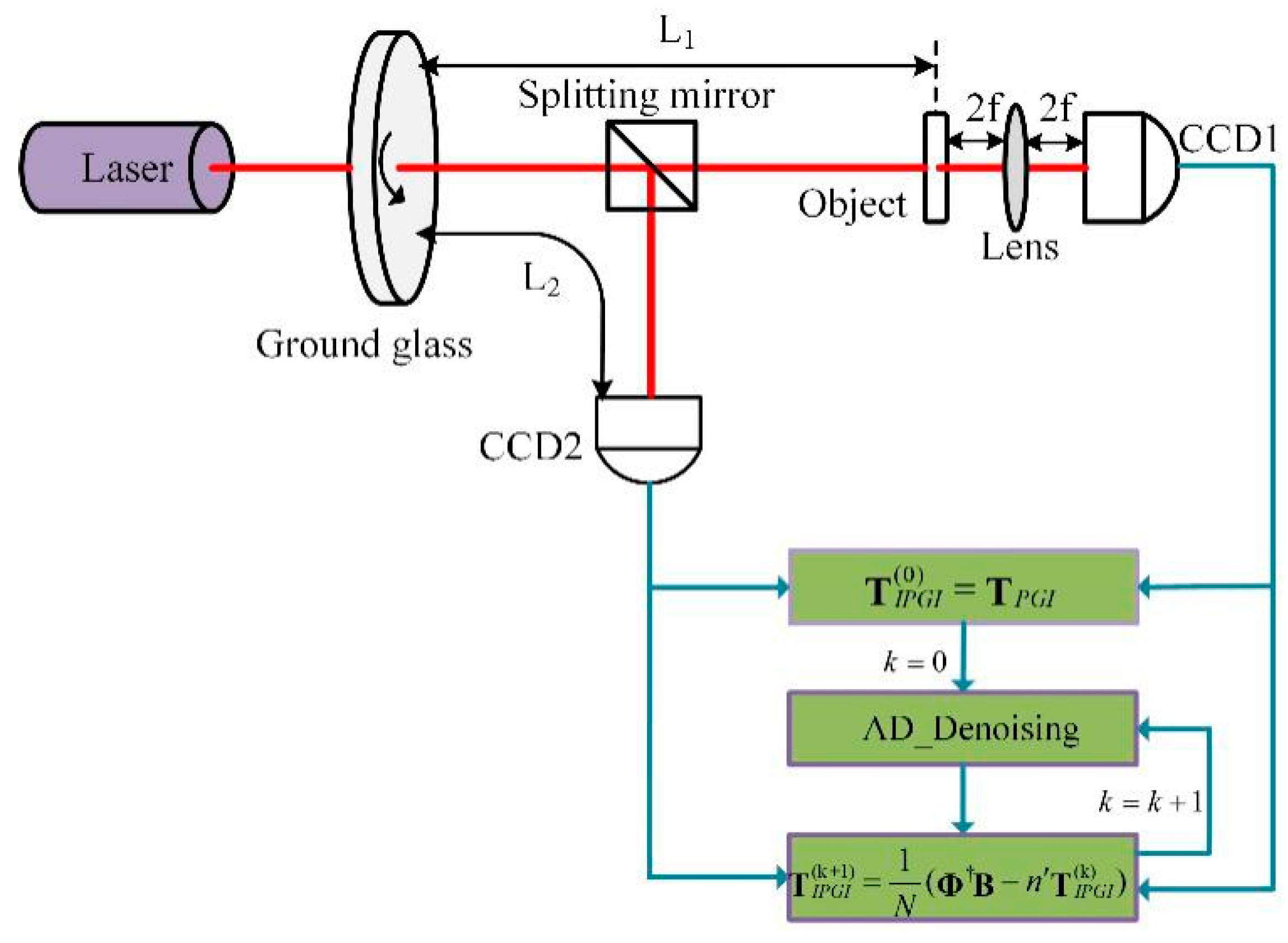
The experimental schematic is shown in
Figure 1; the pseudo-thermal light source is generated by a beam of the laser (with wavelength
= 650 nm) irradiating a rotating ground glass. The beam is then divided into the reference beam path and the object beam path by a 50:50 beam splitter. In the object beam path, the total light intensity of scattered light or transmitted light after a beam of light irradiated an object is collected by CCD1, and the nth measurement value is denoted as Bn. The transfer function of the measured object is
. At the same time, the optical intensity distribution of the other beam is recorded by the CCD2 in the reference beam path, and the nth measurement value is denoted as
. PGI uses these sampled data to reconstruct objects and the reconstructed results are recorded as
, the initial image of IPGI.
firstly is smoothed by anisotropic diffusion (denoted as AD_ denoising in short as shown in
Figure 1), then the denoised image is used to construct the noise interference item of IPGI. Finally, the noise interference term is substituted into the equation of IPGI for iterative computation. Theoretically, the reconstructed result of the current iteration is clearer than the previous iteration, so the reconstructed image of the current iteration can be used to construct the noise interference term of next iteration after denoised by AD_ denoising, which is much closer to the actual noise term.
Anisotropic diffusion, combining the image filtering process with the image edge detection process, shows better performance than that of the traditional denoising methods. Suppose the initial image before denoising is
u (x, y); the time variable t is introduced to represent the changing process of the image and the change of the image can be expressed as a partial differential equation:
where
F represents an operator corresponding to a particular algorithm. The solution to the equation
u (
x, y, t) denotes the image at time
t. The anisotropic diffusion equation is expressed as:
where div and
are respectively denoted as the divergence operator and the gradient operator.
is the length of the gradient
, and it plays an important role in determining if the current region is a smooth or edge area. If the current region is a smooth one, the value of
is small and the diffusion ability will be intensified. On the contrary, the opposite happens when the current region is an edge region. The term
is the diffusion coefficient, which meets the following conditions:
is a monotonically decreasing function and .
denotes that the diffusion is enhanced in the smooth area and shows that the diffusion is stopped in the edge area.
According to the nature of
, its specific expression is presented as follows:
where
m is an artificial parameter, and its value plays an important role in image denoising. When
, the diffusion ability is strengthened, and the image has a good effect of denoising; otherwise, the diffusion coefficient is suppressed but the edge information will be well preserved. However, choosing too small an
m will result in excessive smoothing, even blurring of the image, but too large an
m will cause the image to stop spreading in advance, which may make the denoising effect worse. Therefore, giving a suitable value of
m can make the processed image have good denoising performance, and more features can be extracted from the edge details.
In image processing, the image is considered as a group of pixels, and the diffusion process occurs when computation is conducted among the target pixel with its four adjacent pixels. Therefore, Equation (2) can be transformed into the following form by the nonlinear discrete transformation:
where the discrete time variable t can be used to represent the number of diffusions, 0 ≤ λ ≤ 1/4 must be satisfied for the numerical scheme to be stable, N, S, E and W are abbreviations for north, south, east and west, respectively, which are utilized to expressed the four nearest-neighbor directions of the diffusion, and the gradient functions in the four directions can be expressed as follows:
The diffusion coefficients in the four directions are expressed as:
In the following experiment, considering the balance between eliminating noise and protecting edges, we set the thermal conductivity coefficient
m to 15, the smoothing coefficient λ to 0.15 and the diffusion time
t is set to 20 [
30].
Assuming that the measurement times are
N, the object image and the optical fields distribution of the reference beam are both
pixels. The
consists of a row vector, and then these
N row vectors are pieced together into a matrix expressed as an observation matrix
and the Bn measurements of
N times constitute an
N-dimensional column vector B. The GI formula can be expressed in the form of a matrix:
where the
denotes the ensemble average of the values in the symbol and T equals
. As the number of measurement times increases, the second term in Equation (1) tends to be a constant and barely affects the quality of the reconstructed image, so it can be deleted. Since the closer
is to the scalar matrix, the better reconstruction results will be obtained, and the pseudo inverse matrix
is replaced by PGI. PGI replaces
with its pseudo-inverse matrix.
where the matrix
can be expressed as the sum of two matrices s and n, where s = diag(
) and n =
− s. Theoretically, when s is close to a scalar matrix and n is similar to a zero matrix, the reconstructed image of PGI will be close to the original image of the object. Therefore, (1/
N) nT is the actual noise in the PGI reconstruction, and its presence obscures the image. IPGI constructs the noise interference term using the reconstructed image of PGI without prior information. The iterative formula of IPGI is expressed as:
where the
and the threshold t varies from min {
n (x, y)} to max {
n (x, y)}. A normalized threshold
is utilized to simplify the experimental analysis [
11,
13].
IPGI requires the initial image to be as clear as possible, otherwise the constructed noise interference terms may deviate from the actual noise and more noise will be generated after iterative operations. Although the reconstructed image of PGI, chosen as the initial image of IPGI, is clearer than that of other methods, it still has a lot of background noise. Anisotropic diffusion can solve the problem well; it adapts to both the image and the noise, and balances the tradeoff of noise removal versus preserving the image details. Therefore, our method has improved Equation (9) by combining anisotropic diffusion with IPGI; it is expressed by the Equation (11):
where
is the kth iterative result of IPGI, “0” means it is also the initial image before anisotropic diffusion denoising,
is the result of anisotropic diffusion smoothing of
, and the number of diffusions equals
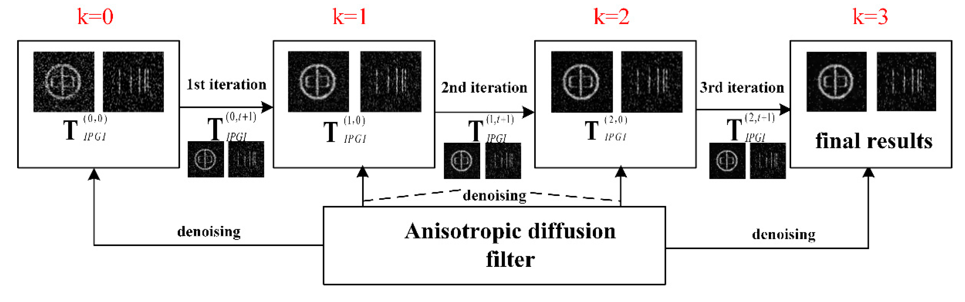
t+1. The imaging process of our method is shown in
Figure 2. The reconstructed results of PGI, denoted as
, are chosen as the initial image of IPGI, then
, the result of anisotropic diffusion smoothing of
, is used to construct the noise interference term of the first iteration.
After the first iterative computation, the reconstruction result
is obtained. By repeating the computation method, the reconstructed image with less noise and better edge details can be obtained after several iterations. We verified the experiment results and found that the best quality reconstructed image produced by the IPGI process was achieved when the iterative times k was equal to 3 [
10].
3. Experiments and Discussion
To verify the effectiveness of our method, a series of experiments were performed using the setup shown in
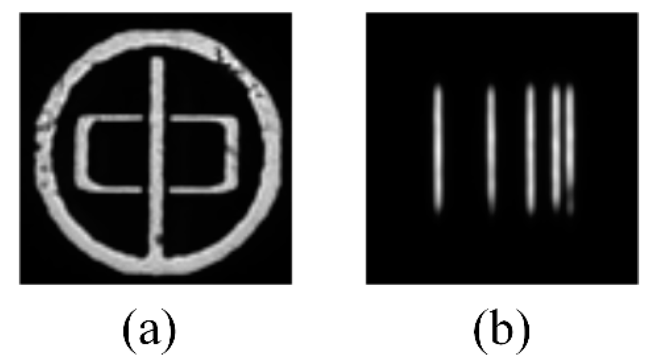
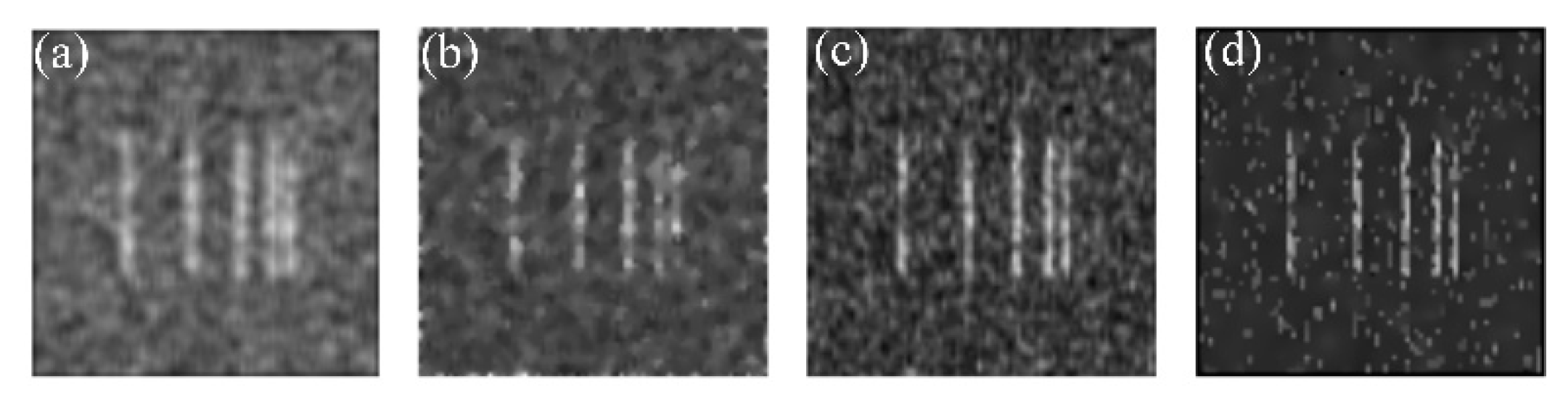
Figure 1. Given that IPGI has a fine ability of image reconstruction, the number of experimental samples was small, less than 6400 groups. In the first set of experiments, we choose a binary transmission aperture “Zhong” (shown in
Figure 3a)as the reconstructed object, the distance L
1 (L
1 = L
2) was 200 mm, the focal length f of the lens was 150 mm and the speckle transverse size was 40 μm. CCD1 and CCD2 were identical devices (Stingray F-504B, AVT, Stadtroda, Germany), however, their roles in the experiment are completely different: CCD1 is used to gather the sum of light field distribution when the object beam has been modulated, while CCD2 is used to record the light field distribution of the reference beam at the surface of the measured object. For a simple illustration, the method of combining anisotropic diffusion with IPGI is abbreviated as AD-IPGI.
The peak signal-to-noise ratio (PSNR) is introduced as a quantitative measurement of the similarity between the reconstructed image and the original image, to evaluate the method more objectively. It is defined as:
where
indicates that the maximum pixel value of the grayscale image, the range of pixel values is from 0 to 255, and MSE represents the mean square error between the original image and the reconstructed image.
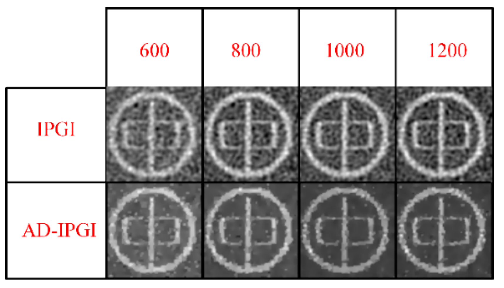
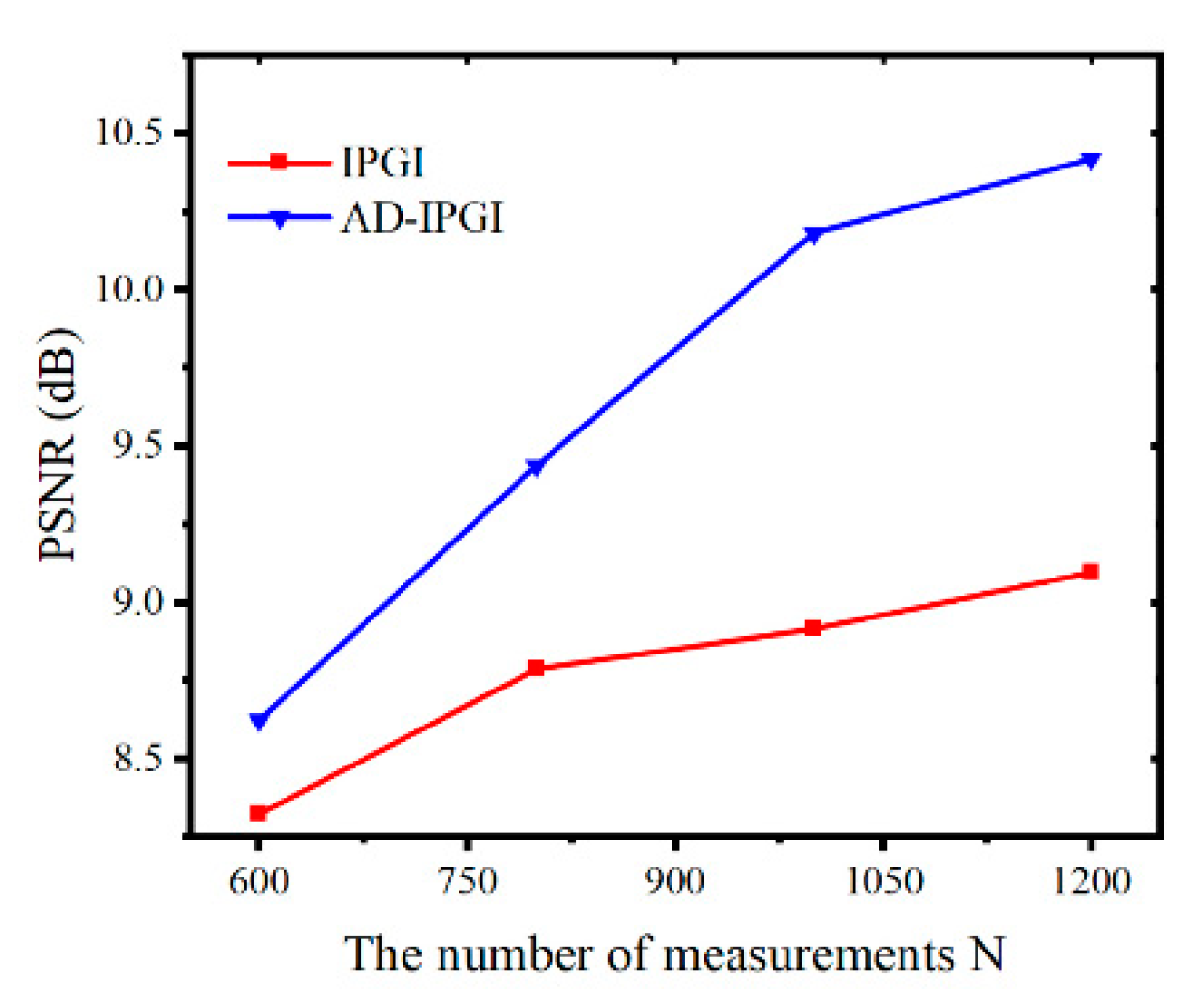
As shown in
Figure 4 and
Figure 5, with the increase of measurement times, the visual effects of the reconstructed images of IPGI and AD-IPGI are synchronously enhanced, their PSNR also respectively rises to varying degrees, but the PSNR of IPGI rises slowly, and there is so much background noise in its reconstructed images, even some information of the imaging object “Zhong” is submerged by the background noise with the sampling time of 600. Instead, we can see an obvious enhancement of both the visual effect and the PSNR of the reconstructed image of AD-IPGI over that of IPGI at the same sampling times. The noise of AD-IPGI results is reduced and the imaging quality is increased greatly after the anisotropic diffusion process. The edges can be well preserved in reconstructed images of AD-IPGI, even at the measurement time of 600. The experimental results show the effectiveness of our method.
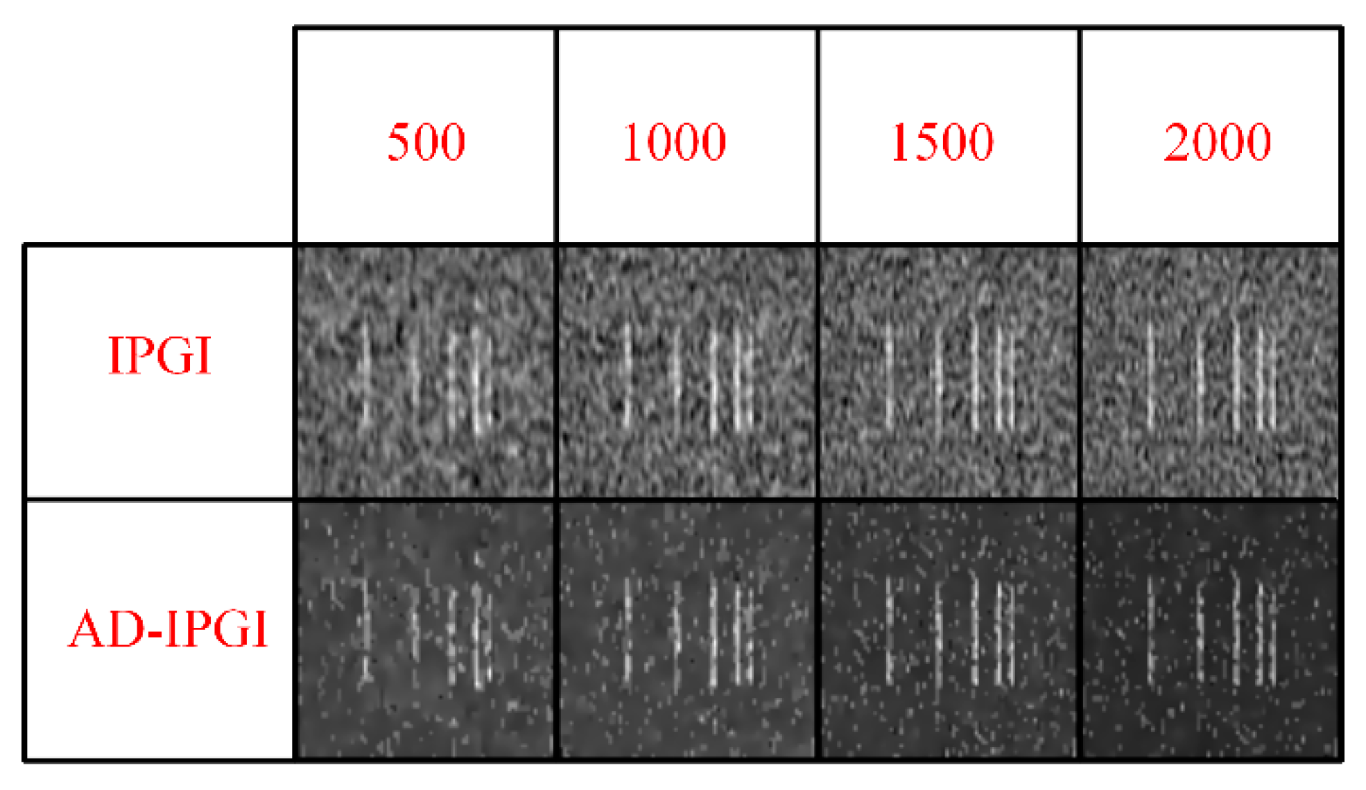
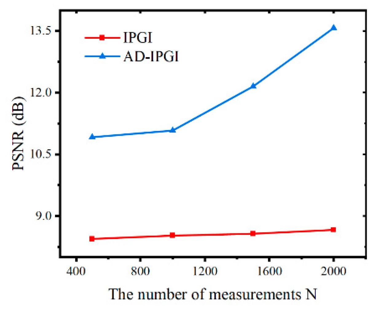
Our method performs better in experiments with smaller speckle transverse size. This is because the size of noise points and speckle are similar in ghost imaging experiments, and the isolated smaller noise points in the original images can be removed more effectively by anisotropic diffusion, making the constructed noise disturbance closer to the actual noise with the edges well preserved. In the second set of experiments, we chose imaging object “Slits” (shown in
Figure 3b) as the reconstructed object. The experimental parameters depicted in
Figure 1 are as follows: L
1 = L
2 = 150 mm, f = 250 mm, and the speckle transverse size is 19.5 μm. Experimental results are shown in
Figure 6 and
Figure 7, where the reconstruction images of IPGI are filled with massive background noise. Some imaging information may be masked by the background noise at fewer measurement times, such as the detail loss of the two stripes on the right side in the IPGI result; the detail loss is serious at 500 groups of data. Under the same conditions, AD-IPGI has better performance on “Slits” imaging. As shown in
Figure 6, AD-IPGI reduces the noise and strengthens the visual effects effectively. The PSNR of the AD-IPGI improved significantly while the PSNR of the IPGI has not changed much with the increased number of measurements. The PSNRs of AD-IPGI are 2.5, 2.6, 3.6 and 4.9 dB higher than those of the IPGI image results for 500, 1000, 1500, and 2000 measurements, respectively. The above experiments have shown that the method can further improve the imaging quality and both the visual effect and PSNR of the reconstructed image are better than those of IPGI; at the same time, the edge details of the image are well preserved.
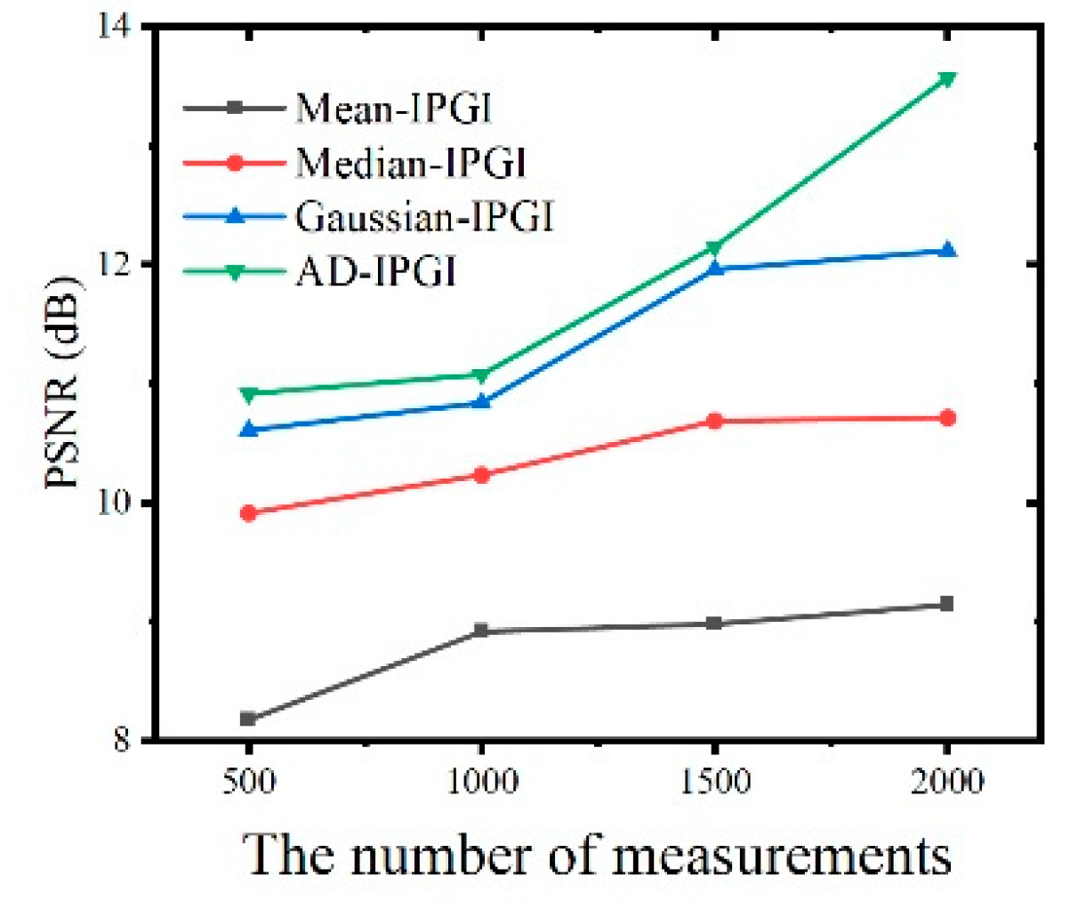
To explain why we choose anisotropic diffusion instead of other filtering methods, the common filtering methods median filter, mean filter and Gaussian filter are combined with IPGI separately to smooth the images used to construct the noise interference term before each iterative operation in the third set of experiments. These three methods are respectively abbreviated as Mean-IPGI, Median-IPGI and Gaussian-IPGI. The experimental results are shown in
Figure 8 and
Figure 9. Compared with IPGI, the reconstruction results of these four methods are improved to various degrees, which again proves the importance of image denoising before each iteration. As
Figure 8 and
Figure 9 show, Mean-IPGI can partially filter the background noise, but at the same time, it makes the image details blurred. Median-IPGI can protect the sharp edges of the image, but the denoising effect is poor. Compared with Mean-IPGI and Median-IPGI, the reconstruction quality of Gaussian-IPGI is much better and the details are well preserved. However, there is always a gap between the Gaussian-IPGI and AD-IPGI on denoising capability. Moreover, the three methods above are only applicable to certain types of noise, while anisotropic diffusion has a more general usability. The PSNR curves in
Figure 8 are consistent with the analysis of visual effect.


