Precision Analysis and Error Compensation of a Telescope Truss Structure Based on Robotics

Abstract

We propose a new secondary mirror support structure assisted by multi-robotics to improve the observation performance of vehicle-mobile telescope systems. A mathematical model of the displacement at the end of the robotic and the variation of telescope pitch angle is established, then the posture of the robotic is optimized by the Jacobian matrix iteration inverse kinematic problem method. Based on the new support structure, a high-order sensitivity matrix is proposed to establish the mapping relationship between the robotic misalignment and the Zernike coefficient, with the accuracy verified via the Monte Carlo method. The method of adjusting the secondary mirror to compensate the aberration caused by the primary mirror is proposed, and the relationship between the primary mirror surface error and the system error is established under different pitch angles before and after compensation. The experiment and simulation results showed that the adjustment calculated by the high-order sensitivity matrix method can effectively compensate for the misalignment caused by the robotics and the primary mirror surface error to a certain degree. After multiple iterations, the root mean square of the wavefront aberration was better than $\lambda /15$. This conclusion provides an engineering application reference value for the secondary mirror support and aberration correction technology of the vehicle telescope system.

1. Introduction

Owing to the versatility offered by their mobility, vehicle-mobile telescopes are a useful observation tool for astronomers, the military, and in other fields. However, owing to the transport-related restrictions on the height and volume of the vehicle-mobile telescope, traditional vehicle-mobile telescopes have a meter-scale aperture. At present, the maximum aperture of the vehicle-mobile telescope system is 1.2 m. To a certain extent, this limits light-gathering ability, resolution, and observation ability of vehicle-mobile telescopes [1,2,3,4,5,6].

The secondary mirror (SM) of the telescope is fixed principally to the Serrurier truss through the Stewart platform for position error adjustment and correction. The Serrurier truss occupies half of the height space of the telescope system, representing the main obstacle preventing caliber improvements for vehicle-mobile telescopes [7,8,9,10]. To solve this issue, this paper proposes an SM truss structure based on parallel robotics to replace the traditional Serrurier truss, enabling the telescope to be adapted depending on whether the observation state or the transport state is required. This structure can provide space for a larger-caliber telescope system, thus improving the observation performance of the vehicle-mobile telescope while satisfying transportation requirements [11,12,13,14,15,16].

As the aperture of the telescope increases, misalignment errors of the primary and secondary mirrors caused by structural gravity, rigid displacement of the supporting structure, thermal deformation, and other factors also gradually increase, which reduces the imaging quality; therefore, correction of these misalignment errors is necessary. In terms of offset error correction, the European Southern Observatory used correction technology based on active optics for the first time on the New Technology Telescope (NTT) [17], but the active support technology of the primary mirror is difficult to apply in vehicle-mobile telescopes. Elsewhere, Lucimara et al. analyzed the sensitivity of the third-order coma of the two-reflection system to off-center [18]. In addition, Soenghui Kim used the inverse optimization method to adjust a Cassegrain telescope, thereby adjusting the wavefront aberration from 0.283$\lambda$ to 0.194$\lambda$ [19]. Using nodal aberration theory, Fuerschbach studied the aberration type corresponding to the free-form surface type located at any position in the system [20]. However, the adjustment range in these methods is small, and the adjusted wavefront aberration cannot meet the requirements in this case.

In order to achieve a larger aperture in a vehicle-mobile telescope under the conditions required for road transportation, this paper proposes a novel robotic SM support structure, which optimizes the posture of the robotics via the stiffness performance index to reduce the misalignment of the SM. Then, using high-order sensitivity matrices, the mapping relationship between the misalignment of the SM and the Zernike coefficient is established. In addition, the wavefront aberration caused by the shape of the primary mirror (PM) under the influence of gravity and the compensation ability of the SM are analyzed quantitatively. Finally, the feasibility of the method is verified experimentally.

2. Structural Analysis of the Telescope Manipulator Based on Stiffness Performance Index

In order to realize vehicle-mobile telescopes with larger apertures and satisfy the requirements of road transportation, this paper proposes a robotic SM truss structure, as shown in Figure 1. In the observation state, the SM is placed at the designated position for observation, as shown in Figure 1a. When the telescope needs to be transported, a robotic arm will place the SM on the side of the telescope, as shown in Figure 1b. This truss structure makes it possible to realize larger-aperture vehicle-mobile telescopes.

The optical system is very sensitive to adjustment errors. Taking the Ritchey-Chrétien (RC) system as an example, the distance adjustment between the PM and SM causes defocusing, while off-centering and tilt produce coma. Therefore, it is necessary to conduct an error analysis for the new SM truss mechanism. As the surface error of the SM is negligible, the error introduced by the SM system can be regarded as the misalignment caused by gravity in an ideal optical system, which manifests as displacement at the end of the robotic arm. Therefore, in order to optimize and verify the influence of the new SM truss structure on the optical system, the final error is evaluated only after optimizing the stiffness of the truss structure.

The robot stiffness depends on the following factors: (1) geometric and material properties of the links, (2) actuators and other transmission elements, and (3) robot postures. Usually, for a given manipulator, the factors (1) and (2) two are almost the same; therefore, this aims to optimize the misalignment of the SM by adjusting the posture [21].

2.1. Optimization Principle

Assuming that the connecting rod of the robot arm is a rigid body, the main reason for the deformation of the robot arm comes from the joints. Each joint can be regarded as a linear spring body. Thus, by connecting the SM to the end of the robot arm, the displacement of the SM can be passed through the robot arm. The displacement at the end is as follows:

$$\mathsf{\Delta }{x}_g=Cw,$$

(1)

where $\mathsf{\Delta }{x}_g$ and $Cw$ represent the generalized displacement and generalized force, respectively. $C$ is a $6\times 6$ flexibility matrix,

$$C=J{K}_{\theta }^{-1}{J}^T=\left[\begin{array}{cc}{C}_{tt}& C_{tr}\\ C_{tr}^T& C_{rr}\end{array}\right],$$

(2)

and $K_{\theta }$ is the joint stiffness matrix of the robotic arm, defined as

$$K_{\theta }=\left[\begin{array}{cccc}{k}_1& 0& \cdots & 0\\ 0& k_2& \cdots & 0\\ ⋮& ⋮& \ddots & ⋮\\ 0& 0& \cdots & k_6\end{array}\right].$$

(3)

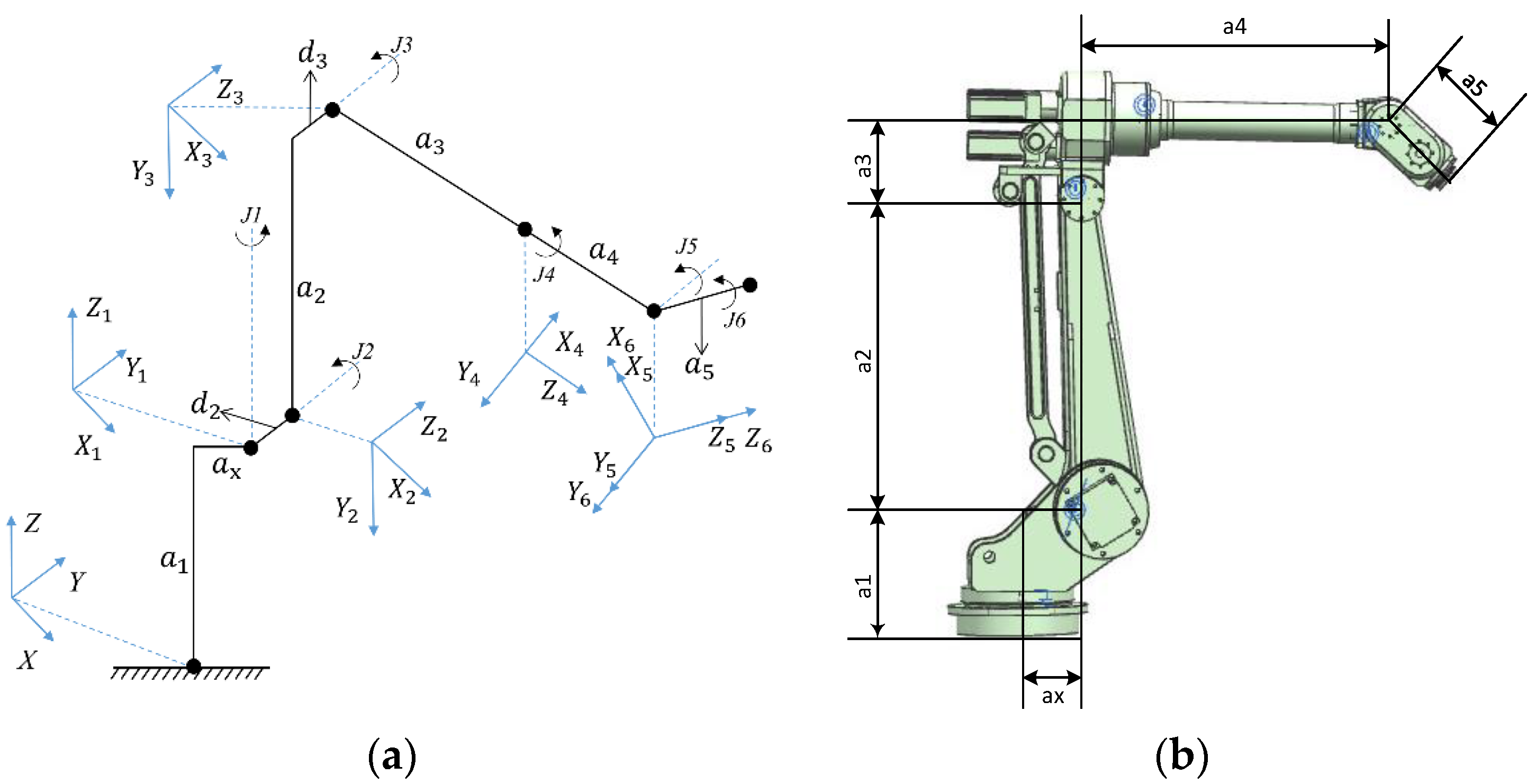
Owing to the constraints of the distance between the PM and SM, we selected the FANUC Robot M-20iA/12L as the research object. The corresponding $K_{\theta }$ can be expressed as diagonal matrix $(5.88\times {10}^8$, $5.36\times {10}^8$, $2.71\times {10}^8$, $2.12\times {10}^8$, $1.22\times {10}^8$, $1.06\times {10}^8$) ($N\cdot mm/rad$).

$J$ is the Jacobian matrix of the robotic manipulator. We established the coordinate system of each joint for the selected manipulator, as shown in Figure 2. Then, the Denavit–Hartenberg parameters (DHm) can be obtained, as shown in

Table 1. Denavit–Hartenberg (DHm) parameters of the robot in the research case.

	J1	J2	J3	J4	J5	J6	x
${\theta }_i \left(rad\right)$	${\theta }_1$	${\theta }_2$	${\theta }_3$	${\theta }_4$	${\theta }_5$	${\theta }_6$	0
${\alpha }_i \left(deg\right)$	−90°	0°	−90°	90°	−90°	0°	0
$a_i \left(mm\right)$	525	790	250	1190	100	0	150
$d_i \left(rad\right)$	0	132	132	0	0	0	0

.

Considering the slow motion of the telescope during observation, it can be regarded as a quasi-static process. The acceleration can be ignored, and only the influence of gravity is considered. Therefore, the force at the end of the truss can ignore the influence of the moment on the system, and only the translation needs to be considered. Therefore, the displacement of the SM can be expressed as:

$$\left[\begin{array}{c}\mathsf{\Delta }X\\ 0\end{array}\right]=\left[\begin{array}{cc}{C}_{tt}& C_{tr}\\ C_{tr}^T& C_{rr}\end{array}\right]\left[\begin{array}{c}F\\ 0\end{array}\right]=\left[\begin{array}{c}{C}_{tt}F\\ 0\end{array}\right],$$

(4)

where $F={[\begin{array}{ccc}{F}_x& F_y& F_z\end{array}]}^T$ represents the force applied to the end of the robotic arm. Under the condition of pitching motion, $F$ is composed of the components of gravity of the SM in different directions at different pitch angles of the telescope system. $\mathsf{\Delta }X={[\begin{array}{ccc}\mathsf{\Delta }x& \mathsf{\Delta }y& \mathsf{\Delta }z\end{array}]}^T$ indicates the displacement at the end of the robotic arm. The misalignment of the secondary mirror can be calculated and verified using Equation (4).

For a robotic system, the optimization of the posture can be regarded as the maximization of the stiffness coefficient:

$$k_{stif}=\frac{1}{\sqrt[3]{\mathit{det}(C_{tt})}}=\frac{1}{\sqrt[3]{\mathit{det}(J_{11}{K}_{11}^{-1}{J}_{11}^T+J_{12}{K}_{22}^{-1}{J}_{12}^T)}}.$$

(5)

Among them, $J_{11}$, $J_{12}$ is the 3 × 3 sub-matrix of $J$:

$$J=\left[\begin{array}{cc}{J}_{11}& J_{12}\\ J_{21}& J_{22}\end{array}\right].$$

(6)

$k_{stif}$ is affected by ${\theta }_i$, $a_i$, and ${\alpha }_i$, where $a_i$ and ${\alpha }_i$ are values determined after establishing the coordinate system, and ${\theta }_i$ is the angle between $J_i$ and $J_{i+1}$. The stiffness coefficient has the invariance of coordinate system transformation, and therefore, the optimization model can be expressed as:

$$\{\begin{array}{c}\mathit{max}{k}_{stiff}\\ s.t.T\left(q\right)=T\left(P,N,\theta \right)\\ q_{imin}\le q_i\le q_{imin},1\le i\le 6\end{array},$$

(7)

where $q=\left[\begin{array}{cccccc}{q}_1& q_2& q_3& q_4& q_5& q_6\end{array}\right]$ is a vector composed of the angles, and $T\left(P,N,\theta \right)$ is the pose matrix connected with the SM that contains the elements $P, N, \mathrm{and} \theta$. $T\left(q\right)$ is the pose matrix formed by the kinematic model that corresponds to the end of the robotic arm.

Before optimizing the stiffness coefficient, the initial pose of the robotics must be solved. First, we determined the position vector $P$ and direction vector $N$ of the end of the robotic arm according to the relative positions of the PM and SM; then, the initial pose of the end of the robotic arm is

$$T_0=\left[\begin{array}{cccc}{U}_X& V_X& N_X& P_X\\ U_Y& V_Y& N_Y& P_Y\\ U_Z& V_Z& N_Z& P_Z\\ 0& 0& 0& 1\end{array}\right],$$

(8)

where $P={\left[\begin{array}{ccc}{P}_X& P_Y& P_Z\end{array}\right]}^T, N={\left[\begin{array}{ccc}{N}_X& N_Y& N_Z\end{array}\right]}^T, \mathrm{and} U={\left[\begin{array}{ccc}{U}_X& U_Y& U_Z\end{array}\right]}^T$ is an arbitrary unit vector in the plane perpendicular to $N$, and $V={\left[\begin{array}{ccc}{V}_X& V_Y& V_Z\end{array}\right]}^T$ is the cross product of ${\left[\begin{array}{ccc}{N}_X& N_Y& N_Z\end{array}\right]}^T$ and ${\left[\begin{array}{ccc}{U}_X& U_Y& U_Z\end{array}\right]}^T$.

All the inverse kinematic solutions are solved according to the initial pose of the robot end pose, and the maximum stiffness performance index value is selected to be $q_0$ as the initial joint angle vector.

Then, the inverse kinematic problem (IKP) method based on Jacobian matrix iteration can solve the joint angle of each feasible pose and the maximum stiffness coefficient is selected in the range of $\left[{\theta }_{min},{\theta }_{max}\right]$. The solution process is as follows:

(1) Initial $q=q_0$ (2) $\left\{p,Q\right\}=pk\left(q\right)$ (3) $\Delta p=p_d-p$, $\Delta \alpha ={\alpha }_d{\alpha }^T$ (4) $\Delta \delta =\left[\begin{array}{c}\Delta p\\ vec\left(\Delta \alpha \right)\end{array}\right]$ (5) $\Delta q=J{(q)}^{-1}\Delta \delta$ (6) $q=q+\Delta q$ (7) If $q$ is reachable, go next; Else, go back to (2) (8) Output $k_{stif}=\frac{1}{\sqrt[3]{\mathit{det}(C_{tt})}}$

where $pk\left(q\right)$ represents the positive kinematics solution, $p$ is the real-time position vector of the robotic arm end in the iterative process, $\alpha$ is the rotation matrix representing the real-time posture of the robotic arm end in the iterative process, $p_d$ represents the end target position vector, and ${\alpha }_d$ represents the rotation matrix of the end target pose.

$\mathsf{\Delta }q$ represents a small change in the angle vector, while $\mathsf{\Delta }\delta$ represents a small change in the end posture, and is defined as

$$\mathsf{\Delta }\delta =\left[\begin{array}{c}\mathsf{\Delta }p\\ vec\left(\mathsf{\Delta }\alpha \right)\end{array}\right],$$

(9)

where $\mathsf{\Delta }p$ denotes a small change in position, $\Delta \alpha$ is a small change in the rotation matrix, and $vec\left(\mathsf{\Delta }\alpha \right)$ is the axial vector of $\mathsf{\Delta }\alpha$:

$$vec\left(\Delta \alpha \right)=\frac{1}{2}\left[\begin{array}{c}\mathsf{\Delta }{\alpha }_{32}-\mathsf{\Delta }{\alpha }_{23}\\ \mathsf{\Delta }{\alpha }_{13}-\mathsf{\Delta }{\alpha }_{31}\\ \mathsf{\Delta }{\alpha }_{21}-\mathsf{\Delta }{\alpha }_{12}\end{array}\right].$$

(10)

2.2. Optimization Results

Because the SM truss is a symmetrical parallel mechanism, the form of the parallel compliance matrix can be written as

$$C_{tt}={\left(C_{tt1}^{-1}+C_{tt2}^{-1}+C_{tt3}^{-1}\right)}^{-1},$$

(11)

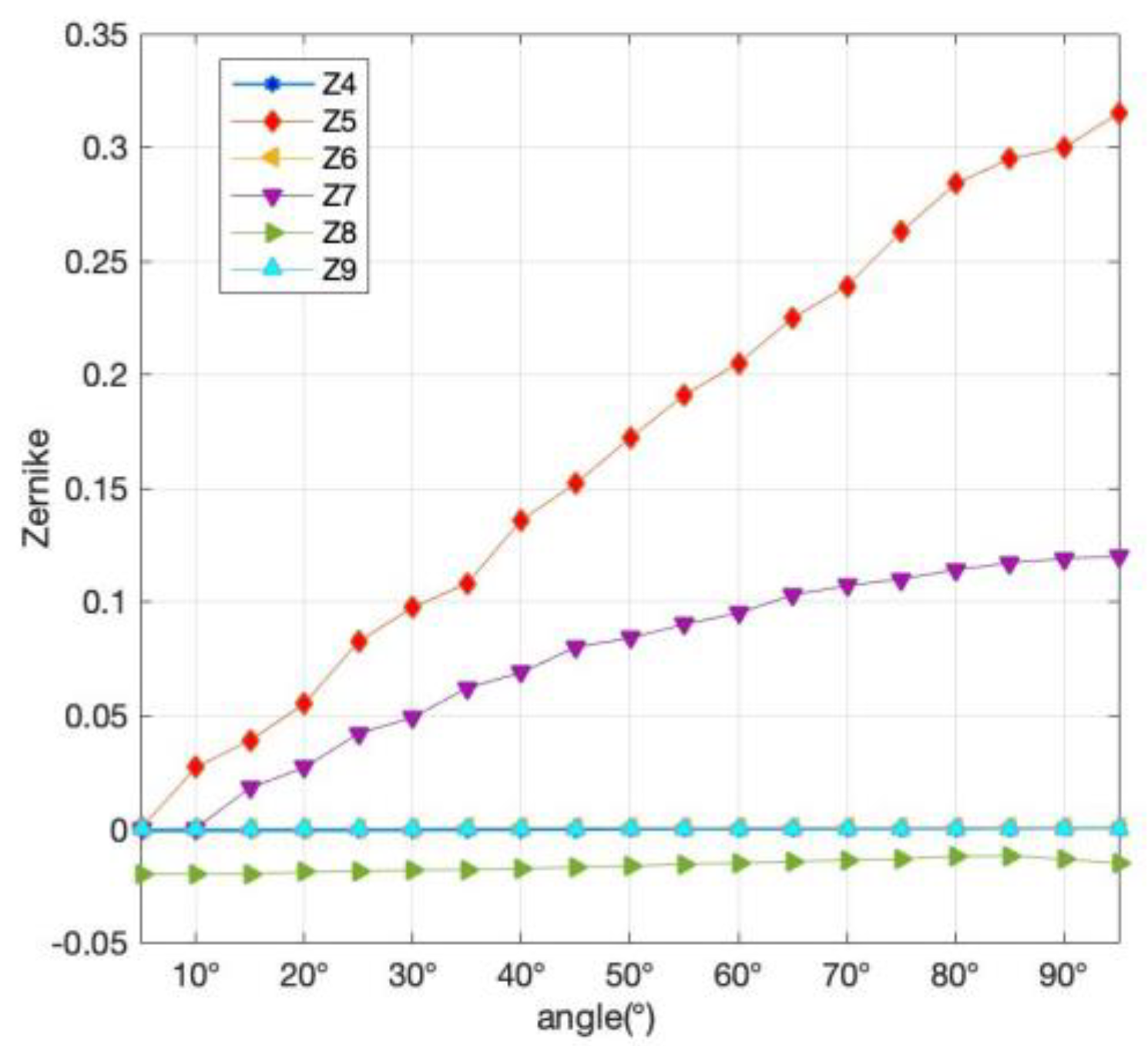
where, $C_1$, $C_2$ and $C_3$ are the flexibility matrices corresponding to the three limbs, respectively. To obtain the optimization of the stiffness coefficient of the manipulator, the calculation results of the parallel compliance matrix are incorporated into Equation (3). The offset components of the SM corresponding to the x-, y-, and z-directions changing with pitch angle in the gravity field are shown in Figure 3.

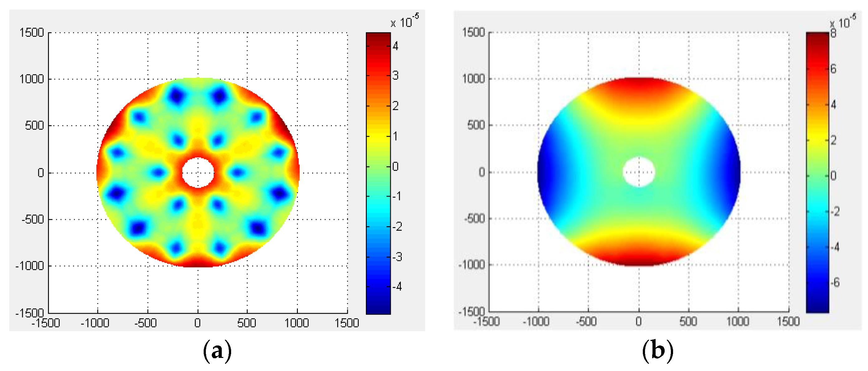
The offsets in the x-, y-, and z-directions are incorporated into the optical system as the offset of the SM, with the wavefront aberration root mean square (RMS) value of the offset system subsequently obtained (see

Table 2. Secondary mirror misalignment and wavefront aberration.

Angle of Optical Axis	0	45°	90°
$\mathsf{\Delta }x \left(mm\right)$	−0.033	0.0276	0.0720
$\mathsf{\Delta }y \left(mm\right)$	−0.018	−0.0064	0.0090
$\mathsf{\Delta }z \left(mm\right)$	0.135	0.0716	0.0338
RMS of wavefront aberration $\left(\lambda \right)$	0.25	0.18	0.48

).

According to the data in Table 2, when the optical axis is vertical, the RMS of the aberration caused by gravity is $0.25\lambda$, and when the optical axis is horizontal, it is $0.48\lambda$. It can be observed that the wavefront aberration caused by the misalignment of the SM owing to the structural deformation has a greater impact on the optical performance. Furthermore, the aberration introduced by the structural deformation changes in real time with the change in the telescope’s pitch angle. Therefore, in order to improve the optical performance of the system, it is necessary to correct the different misalignments corresponding to the next mirror in different situations.

2.3. Feasibility Analysis of the Robotic Truss Structure

The feasibility of the secondary mirror truss based on robotics must be analyzed before studying the adjustment capability and method of the secondary mirror. The proposed parallel mechanism needs to be able to realize the adjustment function of the secondary mirror.

First, we theoretically analyzed the kinematics of the parallel mechanism. The parallel structure proposed in this paper is a 3-6R mechanism. We established the relationship between the screw theory and geometric algebra and analyzed the kinematics characteristic of the parallel mechanism.

According to the definition of the screw theory and geometric algebra, N-dimensional geometric algebra space can be written as the composition of orthogonal groups $\left\{e_1,e_2,\dots e_n\right\}$, screw can be seen as a line vector with a pitch, and the equation of the screw is $r\times S=S^0-hS$, written in Plücker coordinates as $\left(S;S^0-hS\right)$. The screw can then be represented by geometric algebra as:

$$S=v_1{e}_1+v_2{e}_2+v_3{e}_3+b_1{e}_4+b_2{e}_5+b_3{e}_6,$$

(12)

in which $b_1$ is a scalar. The secondary mirror truss structure can be represented as the model shown in Figure 4. We established a coordinate system at the center of symmetry. The fixed platform is set in the XOY plane in Figure 4 and the radius of the fixed platform is r. The moving platform is set on the above.

The moving subspace of the parallel mechanism can be solved after obtaining the moving subspace of each serial. The position vector of each joint is shown in

Table 3. Position vector and twist in a fixed coordinate system.

Position Vector	Coordinates	Twist
$O{M}_1$	$\left[r, 0, 0\right]$	$S_{M_{11}},S_{M_{12}}$
$O{M}_2$	$\left[-\frac{1}{2}r, \frac{\sqrt{3}}{2}r, 0\right]$	$S_{M_{21}},S_{M_{22}}$
$O{M}_3$	$\left[-\frac{1}{2}r,-\frac{\sqrt{3}}{2}r, 0\right]$	$S_{M_{31}},S_{M_{32}}$
$O{A}_1$	$[x_{A_1},y_{A_1},z_{A_1}]$	$S_{M_{13}}$
$O{A}_2$	$[x_{A_2},y_{A_2},z_{A_2}]$	$S_{M_{23}}$
$O{A}_3$	$[x_{A_3},y_{A_3},z_{A_3}]$	$S_{M_{33}}$
$O{B}_1$	$[x_{B_1},y_{B_1},z_{B_1}]$	$S_{M_{14}}$
$O{B}_2$	$[x_{B_2},y_{B_2},z_{B_2}]$	$S_{M_{24}}$
$O{B}_3$	$[x_{B_3},y_{B_3},z_{B_3}]$	$S_{M_{34}}$
$O{C}_1$	$[x_{C_1},y_{C_1},z_{C_1}]$	$S_{M_{15}},S_{M_{16}}$
$O{C}_2$	$[x_{C_2},y_{C_2},z_{C_2}]$	$S_{M_{25}},S_{M_{26}}$
$O{C}_3$	$[x_{C_3},y_{C_3},z_{C_3}]$	$S_{M_{35}},S_{M_{36}}$

.

According to Equation (12), each twist on the first limb can be written as:

$$\begin{array}{c}{S}_{M_{11}}=e_3\\ S_{M_{12}}=e_2+r{e}_6\\ S_{M_{13}}=e_2-z_{A_1}{e}_4+x_{A_1}{e}_6\\ S_{M_{14}}=e_1+z_{B_1}{e}_4-y_{B_1}{e}_6\\ S_{M_{15}}=e_2-z_{C_1}{e}_4+x_{C_1}{e}_6\\ S_{M_{16}}=e_3+y_{C_1}{e}_4-x_{C_1}{e}_6\end{array}$$

(13)

The motion subspace of the first limb can be regarded as series of independent kinematic pairs on the limb, then the union of the twists is:

$$S_{M_1}=S_{M_{11}}{\displaystyle \cup }{S}_{M_{12}}{\displaystyle \cup }{S}_{M_{13}}{\displaystyle \cup }{S}_{M_{14}}{\displaystyle \cup }{S}_{M_{15}}{\displaystyle \cup }{S}_{M_{16}}=a{e}_1\bigwedge e_2\bigwedge e_3\bigwedge e_4\bigwedge e_5\bigwedge e_6,$$

(14)

Similarly, the motion subspace of the second limb is the union of the twists:

$$S_{M_2}=S_{M_{21}}{\displaystyle \cup }{S}_{M_{22}}{\displaystyle \cup }{S}_{M_{23}}{\displaystyle \cup }{S}_{M_{24}}{\displaystyle \cup }{S}_{M_{25}}{\displaystyle \cup }{S}_{M_{26}}=b{e}_1\bigwedge e_2\bigwedge e_3\bigwedge e_4\bigwedge e_5\bigwedge e_6,$$

(15)

The motion subspace of the third limb is the union of the twists:

$$S_{M_3}=S_{M_{31}}{\displaystyle \cup }{S}_{M_{32}}{\displaystyle \cup }{S}_{M_{33}}{\displaystyle \cup }{S}_{M_{34}}{\displaystyle \cup }{S}_{M_{35}}{\displaystyle \cup }{S}_{M_{36}}=c{e}_1\bigwedge e_2\bigwedge e_3\bigwedge e_4\bigwedge e_5\bigwedge e_6,$$

(16)

$a,b,c$ are scalars in the equations that do not influence the result. It can be obtained from the calculation that the motion subspace of each limb at the end of the kinematic chain is a 6-blade. N-dimensional geometric algebra comprises a 0-n order blade and the blade of 0 order is a scalar. Then, it is easy to obtain the following equation:

$$S_M=S_{M_1}{\displaystyle \cap }{S}_{M_2}{\displaystyle \cap }{S}_{M_3}=m{e}_1\bigwedge e_2\bigwedge e_3\bigwedge e_4\bigwedge e_5\bigwedge e_6,$$

(17)

$m$ can be calculated by Equations (14)–(16), and m is a scalar that does not influence the result. It can be seen from the calculation that the parallel mechanism of the 3-6R structure has a 6 degrees of freedom adjustment function. Thus, the mechanism meets the requirement of secondary mirror adjustment.

Second, we have built the model of the robotics in Matlab. The Denavit–Hartenberg parameters of the FANUC Robot M-20iA/12L selected in the paper were written into the program, and the parameters were normalized to analyze the workspace of the robot truss structure.

Through the Monte Carlo method, we sampled each manipulator 10,000 times within the motion range of each axis to generate the workspace shown in Figure 5.

The following conclusions can be drawn according to the generated workspace:

• Each mechanical arm can meet the requirements of placing the secondary mirror at a specified position for observation when the telescope is working and placing the robotic arm and secondary mirror on the side of the telescope when the telescope is in transportation.
• The intersection of the workspace is the theoretical position that the three robotic arms can reach at the same time. The range of the secondary mirror adjustment (the range of

  Table 4. Optical system parameters.

  Optical Surface	Radius of Curvature (mm)	Material	Aspheric Coefficient	Radius
  Primary mirror	5500	SiC	K = −1	1000
  Secondary mirror	1051.5	Zerodur	K = −1	166

  ) is very small when the telescope is working compared to the workspace of the robotic arms. The robotic truss can work together to realize the small adjustment of the secondary mirror.

Finally, the values of the 18 joints on the robotic arms have been solved by inverse kinematics according to the displacement of the secondary mirror. The given displacement is the maximum secondary mirror adjustment set in the text. A definite solution can be obtained which proves that the parallel mechanism used in this paper can achieve cooperative work and complete the requirements of secondary mirror adjustment. The joint movements of the three robotic arms are shown in Figure 6.

According to the calculation results above, the robotic truss can realize the function of switching from the transportation state to the working state. The adjustment function of the secondary mirror can be realized by the parallel mechanism as well.

3. Aberration-Compensation Method

The Cassegrain telescope parameters considered in this study are listed in Table 4.

The light path is shown in Figure 7. From Table 2 and Figure 3, it can be seen that although the offset produced by the truss is small, the system aberration is very sensitive to the misalignment of the secondary mirror, and the aberration changes caused by the pitching movement are obvious. In addition, every time the robotics change from the transport state to the working state, an assembly error will also occur. Therefore, this study introduces a second-order compensation term to the sensitivity matrix to adjust the SM in order to compensate for the offset due to different pitch angles and the positioning error during assembly. The repeatability of the robotic arm utilized in this study is 0.03 mm, which guarantees its adjustment accuracy. Considering the scope of the misalignment of the secondary mirror and environmental factors in actual work, such as wind load and temperature, will have a significant impact on the truss. In order to ensure the effectiveness of the compensation in the case of large offsets, the misalignment range of the SM is set in the analysis and modeling (see

Table 5. Secondary mirror misalignment range.

$\mathit{x} \left(\mathit{m}\mathit{m}\right)$	$\mathit{y} \left(\mathit{m}\mathit{m}\right)$	$\mathit{z} \left(\mathit{m}\mathit{m}\right)$	$\mathsf{\Delta }\mathit{\alpha } (°)$	$\mathsf{\Delta }\mathit{\beta } (°)$
$\pm 2$	$\pm 2$	$\pm 2$	$\pm 1$	$\pm 1$

).

The traditional aberration compensation method uses the difference quotient to analyze the linear equations of the Zernike coefficient and the misalignment to obtain the sensitivity matrix. If the Zernike coefficient is a continuous linear function in the misalignment interval, as shown in Figure 8a, the accurate adjustment can be calculated according to the sensitivity matrix. But, some Zernike coefficients show a significant non-linear relationship with the adjustment error, as shown in Figure 8b,c.

In this case, the traditional sensitivity matrix model causes the equation to converge slowly and cannot obtain an accurate solution because of the coupling between the Zernike coefficient and the offset. To solve this problem, this study reduced the nonlinearity of the Zernike coefficient and the offset function that characterizes wave aberration by adding a second-order correction term to the mathematical model of the sensitivity matrix method.

3.1. Principle of Second-Order Sensitivity Matrix

When the optical system is in a misaligned state, the i-th fringe Zernike coefficient, $Z_i$, representing the wavefront aberration of the exit pupil of the j-th field of view can be expressed by the Taylor expansion as follows:

$$Z_i^{\left(j\right)}\left(U\right)=Z_i^{\left(j\right)}\left(N+\Delta M\right)={\displaystyle \sum }_{p=0}^m\frac{1}{p!}{({\displaystyle \sum }_{q=1}^n\mathsf{\Delta }{m}_q\frac{\partial }{\partial x_q})}^p{Z}_i^{\left(j\right)}\left(N\right)+R_{N,m}\left(\mathsf{\Delta }M\right),$$

(18)

where $N=\left(x_{01},x_{02},\cdots ,x_{0n}\right)$ is the design state of the n adjustment degrees of freedom of the optical system, $\mathsf{\Delta }M=\left(\mathsf{\Delta }{m}_1,\mathsf{\Delta }{m}_2,\cdots ,\mathsf{\Delta }{m}_n\right)$ is the misalignment amount on the n adjustment degrees of freedom, and $R_{N,m}\left(\mathsf{\Delta }M\right)$ is the expansion remainder.

Then, the second-order expansion of Equation (12) can be expressed as:

$$\begin{array}{c}{Z}_i^{\left(j\right)}\left(N+\mathsf{\Delta }M\right)=Z_i^{\left(j\right)}\left(N\right)+({\displaystyle \sum _{q=1}^n}\mathsf{\Delta }{m}_q\frac{\partial }{\partial x_q})Z_i^{\left(j\right)}\left(N\right)+\\ \frac{1}{2}{({\displaystyle \sum _{q=1}^n}\mathsf{\Delta }{m}_q\frac{\partial }{\partial x_q})}^2{Z}_i^{\left(j\right)}\left(N\right)+R_{N,2}\left(\mathsf{\Delta }M\right)\approx Z_i^{\left(j\right)}\left(N\right)+\\ {\displaystyle \sum _{q=1}^n}\mathsf{\Delta }{m}_q\frac{\partial }{\partial x_q}+\frac{1}{2}{\displaystyle \sum _{q=1}^n}\mathsf{\Delta }{m}_q^2\frac{{\partial }^2{Z}_i^{\left(j\right)}\left(N\right)}{\partial x_q^2}+\frac{1}{2}{\displaystyle \sum _{\begin{array}{c}p,q=1\\ p\ne q\hfill \end{array}}^n}\mathsf{\Delta }{m}_p\mathsf{\Delta }{m}_q\frac{\partial Z_i^{\left(j\right)}\left(N\right)}{\partial x_p}\frac{\partial Z_i^{\left(j\right)}\left(N\right)}{\partial x_q}.\end{array}$$

(19)

Using the ray-tracing method, the derivative quantity in Equation (13) can be replaced by a linear fitting value:

$$\begin{array}{c}{Z}_i^{\left(j\right)}\left(N+\mathsf{\Delta }M\right)=Z_i^{\left(j\right)}\left(N\right)+{\displaystyle \sum _{q=1}^n}\mathsf{\Delta }{m}_q{b}_q+\\ \frac{1}{2}{\displaystyle \sum _{q=1}^n}\mathsf{\Delta }{m}_q^2{a}_{qq}+\frac{1}{2}{\displaystyle \sum _{\begin{array}{c}p,q=1\\ p\ne q\hfill \end{array}}^n}\mathsf{\Delta }{m}_p\mathsf{\Delta }{m}_q{a}_{pq},\end{array}$$

(20)

which can be expressed in the following matrix form:

$$Z_i^{\left(j\right)}\left(N+\mathsf{\Delta }M\right)=\mathsf{\Delta }M·{\left(A_i^{\left(j\right)}\right)}_{n\times n}·\mathsf{\Delta }{M}^T+\mathsf{\Delta }M·{\left(B_i^{\left(j\right)}\right)}_{n\times 1}+Z_i^{\left(j\right)}\left(N\right),$$

(21)

in which

$${(A_i^{\left(j\right)})}_{n\times n}=\left[\begin{array}{ccc}{a}_i^{\left(j\right)}{}_{11}& \cdots & a_i^{\left(j\right)}{}_{1n}\\ ⋮& \ddots & ⋮\\ a_i^{\left(j\right)}{}_{n1}& \cdots & a_i^{\left(j\right)}{}_{nn}\end{array}\right], a_i^{\left(j\right)}{}_{pq}=a_i^{\left(j\right)}{}_{qp}, {(B_i^{\left(j\right)})}_{n\times 1}=\left[\begin{array}{c}{b}_i^{\left(j\right)}{}_1\\ ⋮\\ b_i^{\left(j\right)}{}_n\end{array}\right].$$

The optical design software is used to analyze the random misalignment example of the optical system model with a sample volume of k, i.e., each $Z_i^{\left(j\right)}\left(N+\mathsf{\Delta }M\right)$ can be obtained via ray tracing by each $\mathsf{\Delta }M$, after which we can establish the linear equation system for the quadratic coefficient and the linear coefficient with k equations:

$$\left[\begin{array}{c}{Z}_i^{\left(j\right)}\left(N+\mathsf{\Delta }{M}_1\right)-Z_i^{\left(j\right)}\left(N\right)\\ ⋮\\ Z_i^{\left(j\right)}\left(N+\mathsf{\Delta }{M}_k\right)-Z_i^{\left(j\right)}\left(N\right)\end{array}\right]=M_{k\times \left(\frac{n^2+3n}{2}\right)}{P}_{\left(\frac{n^2+3n}{2}\right)\times 1}.$$

(22)

The minimal norm least squares solution of Equation (16) is

$$P_{\left(\frac{n^2+3n}{2}\right)\times 1}=pinv\left(M_{k\times \left(\frac{n^2+3n}{2}\right)}\right)\times \left[\begin{array}{c}{Z}_i^{\left(j\right)}\left(N+\mathsf{\Delta }{M}_1\right)-Z_i^{\left(j\right)}\left(N\right)\\ ⋮\\ Z_i^{\left(j\right)}\left(N+\mathsf{\Delta }{M}_k\right)-Z_i^{\left(j\right)}\left(N\right)\end{array}\right],$$

(23)

where $pinv(M_{k\times (\frac{n^2+3n}{2})})$ is the M–P generalized inverse of $M_{k\times (\frac{n^2+3n}{2})}$.

In view of the non-linear relationship between the adjustments and the Zernike coefficients, this paper uses the second-order sensitivity matrix method to correct the system wavefront aberration through the adjustment of the secondary mirror in the large offset range shown in Table 3.

3.2. Adjustment Error Compensation Analysis of Simulated Assembly and Adjustment Errors

A 2 m Ritchey-Chretien (RC) system is analyzed as an example for aberration compensation, and the initial RMS design value of the optical system is 0.021$\lambda$. Setting the communication connection in Zemax and Matlab establishes the relationship between the misalignment of the SM and the aberration characteristics. Dynamic data exchange (DDE) interface is used in this paper to realize the real-time data exchange in Zemax and Matlab. First, a randomly distributed sample of misalignment is produced in a uniform distribution in the misalignment range, and each sample model corresponds to an actual misalignment state. Through Zemax ray tracing, the Zernike coefficients corresponding to each set of offsets, $\mathsf{\Delta }M,$ can be obtained. The optical system produces predominantly primary aberrations in the misalignment state, with the result that fringe Zernike coefficients Z4 to Z9 are used for modeling and calculation. Considering factors such as sample size and calculation time, 10,000 samples were randomly generated in the interval of Table 5 according to a uniform distribution to fit the sensitivity matrix model. According to the calculation method of the quadratic and first-order coefficient matrices, a set of multivariate quadratic equations for the misalignment of the SM is established.

The telescope adjustment was simulated using the optical software, 5000 sets of offset vectors were randomly generated in the interval of Table 5 and calculated in Equation (23) to take the ray-tracing result as the true value, and determine the calculation error of the compensation model after calculating the misalignment using the high-order sensitivity matrix. Figure 9 shows the histograms of the fitting error frequency, showing the root mean square error (RMSE) of the fitting of the corresponding Zernike coefficient. The horizontal axis in the figure represents the fitting error, while the vertical axis represents the frequency.

For a two-mirror system, the rotation of the SM around the zero-coma point will introduce astigmatism that is linearly proportional to the field of view without introducing a coma. Therefore, the establishment and verification of the model also needs to consider multiple fields of view, with F (0, 0), F (0, −0.1), and F (0, 0.1) considered in

Table 6. Root mean square error (RMSE) of the Zernike coefficient under multiple fields of view.

	Z4	Z5	Z6	Z7	Z8	Z9
F (0, 0)	0.2039	0.195	0.2343	0.0403	0.0417	0.0023
F (0, −0.1)	0.1991	0.170	0.2257	0.0309	0.0332	0.0021
F (0, 0.1)	0.2032	0.206	0.2329	0.0414	0.0370	0.0051

. After the corresponding adjustment is calculated and applied through the method in Section 3.1, the RMSE of each Zernike coefficient in each field of view can be obtained.

Combining the RMSE between the misalignment state wavefront calculated by the sensitivity matrix for multiple fields of view and the actual wavefront, it can be observed that the high-order sensitivity matrix method maintains high accuracy even when the system misalignment is large and demonstrates good compensation ability with respect to primary aberrations.

3.3. Compensation of the PM Surface Error

For large-aperture telescopes, there are two main reasons for the misalignment of the PM and SM:

(1)

The misalignment of the SM is caused by the deformation of the truss obtained in Table 2. In addition, the deviation of the SM is due to the large span in the height direction of the truss coupled with its large mass.

(2)

The position deviation of the primary mirror is caused by the deformation of the support structure and the surface error of the primary mirror. The influence of the surface error is much greater than the error caused by the support component.

In practice, as the azimuth and pitch angles change, the gravitational field experienced by the PM also changes continuously, resulting in a PM surface error. This is problematic because the PM is difficult to adjust in actual engineering. Therefore, this study uses the finite element method to analyze the surface error of the PM and attempts to use the adjustment of the SM to compensate for the primary aberration to the system caused by the PM [22,23,24,25,26].

The PM model was established using finite element analysis software. A PM with a diameter of 2120 mm was used as the analysis object. The radius of curvature fitted by the mirror was 6000 mm, and the edge thickness of the mirror body was 260 mm. The axial support of the main mirror adopts an 18-point whiffletree support structure, and the lateral support adopts a tangential rod support method. The constraints adopted by the main mirror model are shown in Figure 10.

By changing the loaded gravity to simulate the pitching movement of the PM during operation, the simulation was performed with a resolution of 5°, tracking the movement process of the optical axis from vertical to horizontal. The surface error has been shown in Figure 11.

The original coordinate node value and the node deformation of the PM surface can be obtained using the finite element analysis software. The surface fitting program was compiled by Matlab, with the least square method used to fit the mirror error and the Zernike polynomial decomposition to obtain the RMS value of the mirror shape and the decomposed Zernike polynomial coefficients [27]. The extracted Zernike fringe coefficients of the PM were introduced into the optical system using the Zemax software, and the simulation finally obtained the wavefront RMS and the 4th to 9th Zernike coefficients (Z4–Z9), as shown in Figure 12.

The simulated system wavefront error is calculated using the high-order sensitivity matrix method. The adjustment of each angle can be obtained through the Zernike coefficients of each angle and the high-order sensitivity matrix, and consequently, the amount of compensation required via adjusting the SM. The adjusted Z4–Z9 fringe Zernike coefficients are shown in Figure 13.

Zernike polynomials were used to fit the low-order surface errors of the PM caused by gravity, and analyze the ability of the system to compensate for the surface errors associated with the optical components after adjusting the SM. This leads to the following conclusion: when the misalignment is caused by the relative positions of the PM and SM, the high-order sensitivity matrix method can compensate for the error in the optical system effectively. The RMSEs in F (0,0) are 0.2039, 0.195, 0.2343, 0.0403, 0.0417, and 0.0023, respectively. The sensitivity matrix can compensate for the astigmatism and coma caused by the PM surface error, but the compensation effect is limited.

4. Secondary Mirror Adjustment Experiment

4.1. Construction of the Experimental Platform

An adjustment experiment platform was built to verify the adjustment ability of the SM with respect to the system as well as the accuracy of the sensitivity matrix calculation. In this study, the experimental object is the primary and secondary mirror system of the RC telescope. The experimental system is composed of a PM system, a SM system, a compensator, an interferometer, and a plane mirror. Since the Stewart platform has the same adjustment capabilities as the secondary mirror truss based on robotics, the SM is connected to the SM truss through the Stewart platform, and it is then adjusted through the Stewart platform after the error is calculated. The positioning accuracy of the Stewart platform can reach 30 $\mathsf{\mu }\mathrm{m}$, which is the same as the robotic arm selected in the article. The schematic diagram of the experiment setup is shown in Figure 14.

Since the Stewart platform has the six degrees of freedom adjustment capability, we have proved that the robotic secondary mirror truss also has the same six degrees of freedom adjustment capability as the Stewart platform in Section 2.3. The secondary mirror needs to have the adjustment function of five degrees of freedom in addition to the rotation along the optical axis, so both the robotic secondary mirror truss and the Stewart platform can meet the system requirements. In addition, since the experiment focuses on the correctness of the secondary mirror adjustment strategy, the Stewart platform can be used in the experiment.

When establishing the experimental system, first, place the primary and secondary mirror system in a horizontal position, fix the compensator behind the PM, and adjust the plane mirror and the interferometer simultaneously via the five-dimensional adjustment platform. The convergent spherical wave emitted by the interferometer is subsequently emitted from the simulated focal point after passing through the compensator, before returning to its original path after being reflected by the primary and secondary mirror system, thus forming a self-collimating loop. It should be noted that covering the detection light path can reduce the influence of air flow disturbance to a certain extent.

Due to the offset error of the PM and the SM, the surface error of the PM, and other uncontrollable factors in the experiment, the adjustments obtained in Section 3.2 and Section 3.3 cannot be directly applied to compensate the system wavefront aberration. Therefore, this article uses an interferometer to measure the wavefront aberration of the system. All the error factors can be considered comprehensively, and then the adjustment of the secondary mirror can be solved by the high-order sensitivity matrix method.

When determining the on-axis field of view, the rotational symmetry axis of the PM and SM coincides with the optical axis of the system, and therefore the rotational symmetry axis of the PM must be calibrated to serve as the detection reference for the on-axis field of view wave aberration. For a single parabolic mirror, only the on-axis field of view can achieve aberration-free imaging. Off-axis field of view imaging is affected by astigmatism and coma. Based on this principle, the relative positions of the interferometer and compensator are adjusted to minimize the detected aberration. Then, the detection field of view is the on-axis field of view. The experimental diagram is shown in Figure 15.

4.2. Experimental Results

The field of view is converted by rotating the plane mirror and the interferometer synchronously, enabling the central field of view and the edge field of view of the system to be detected. The measured system aberrations of the three reference field points are shown in Figure 16.

The wavefront fitting Zernike fringe coefficients of the three reference field points were used to inform the established misalignment solution model, with the corresponding compensation amounts required for the SM listed in

Table 7. Compensation amounts for the SM.

$\mathsf{\Delta }\mathit{x} \left(\mathit{m}\mathit{m}\right)$	$\mathsf{\Delta }\mathit{y} \left(\mathit{m}\mathit{m}\right)$	$\mathsf{\Delta }\mathit{z} \left(\mathit{m}\mathit{m}\right)$	$\mathsf{\Delta }\mathit{\alpha } (°)$	$\mathsf{\Delta }\mathit{\beta } (°)$
0.395	–0.423	0.036	0.02	0.05

.

It should be noted that the compensation amounts in Table 7 are ideal calculated values, not adjusted specific values. According to the sensitivity matrix mapping relationship, it can be known that the tolerance in micrometer level has almost no effect on the aberration of the system. The accuracy of the Stewart platform used in the experiment can meet the requirements of the system. The SM was adjusted as directed by the calculated misalignment, with the detection results of the wavefront error associated with the on-axis and edge fields of view relating to the adjusted system wave aberration shown in Figure 17.

Owing to the limitations concerning the adjustment accuracy, it is impossible to adjust to the ideal wavefront state simultaneously. After the first adjustment, the compensation amount required for the SM is recalculated and adjusted. After multiple adjustments, the wave aberration RMS associated with the three fields of view is better than $\lambda /15$, which satisfies the requirements of the system application. Detection results after multiple adjustments is shown in Figure 18. This result shows that the accuracy of the Stewart platform used in this paper can meet the requirements of system adjustment. Therefore, the robot arm with the same accuracy can also achieve the adjustment accuracy of the secondary mirror, which also shows the feasibility of the secondary mirror truss based on robotics.

4.3. Experiment Analysis

It should be noted that this experiment is an a priori experiment. This experiment verifies the correctness of the high-order sensitivity matrix method in the system aberration compensation problem. At the same time, the feasibility of the secondary mirror truss of the robotic arm can be proved to a certain extent with the theoretical calculation and simulation in Section 2. In the experiment, the Stewart platform was used to adjust the SM. After multiple adjustments, the wavefront aberration can be adjusted to $\lambda /15$, verifying the adjustment ability of the SM. Because the robotics-based SM truss achieves the same adjustment ability as the Stewart platform, it also demonstrates a similar adjustment accuracy. Therefore, the experiment verifies the feasibility of the new structure of the SM scheme and verifies its compensation ability regarding the SM misalignment.

According to the results before and after the adjustment, although the high-order sensitivity matrix method can compensate for the wavefront aberration effectively, it does not correlate exactly with the simulated adjustment results presented in Section 3. In practice, the adjustment process requires multiple iterations to achieve an image quality comparable to the initial design of the optical system. There are several significant sources of error, as follows.

First, in principle, the sensitivity matrix method does not involve optical knowledge and aberration theory but applies a mathematical method and uses a data model to fit localized optimal solutions. Therefore, it is not possible to compensate entirely for the aberration of the full field of view point. The sensitivity matrix method only calculates the misalignment amount based on the data of the on-axis field of view modeling, and then adjusts the position of the SM several times to make the axis the upper point aberration and the off-axis aberration of each field of view as consistent as possible with reference to the wavefront aberration of the edge field of view. This is demonstrated by the adjustment experiment (Section 4.2). After the initial adjustment of the position of the SM, the aberration of the on-axis field of view is improved significantly, but the aberration of the edge field of view is still far from the target value.

Second, in terms of processing errors, the error associated with the radius of curvature of the vertex of the PM processing is $\pm 1$ mm, and the wavefront aberration generated by the system is $\lambda /50$ (RMS), with a surface error of $\lambda /40$ (RMS), and the wavefront aberration generated by the system is $\lambda /20$ (RMS). Moreover, owing to the horizontal construction of the optical system, it can be seen from the finite element simulation conclusions in Section 3.3 that the surface error of the main mirror in the vertical state is the largest error source, and the sensitivity matrix method is limited in the extent that it can compensate for the wave aberration caused by the main mirror surface. In addition, the SM also has processing errors and other factors that cause residual aberration of the system and affect the adjustment effect and imaging quality.

Finally, in the actual adjustment process, there are several environmental factors, such as airflow disturbance, vibration, and field of view detection error, that affect the wavefront detection accuracy. These error sources lead to inaccuracies in the Zernike coefficients obtained by the interferometer, thereby increasing the error in the solution of the offset. The adjustment mechanism is limited by the adjustment accuracy, which will also impact the influence of computer-aided adjustments. Therefore, it needs to make many adjustments to obtain the optimal wavefront state during the actual adjustment.

5. Conclusions

In this study, an SM truss structure based on robotics was proposed and analyzed in order to solve the transport-related limitations involving vehicle-mobile telescopes. The misalignment of the secondary mirror was minimized through the IKP method of Jacobian matrix iteration. The finite element analysis method was used to fit the node displacements of the surface under the gravitational field, and a PM surface error model considering the optical axis from the horizontal to the vertical orientations was established. The high-order sensitivity matrix method was used to effectively compensate for the wavefront aberration of a telescope with large misalignment. Verified through experiments and simulations, our results showed that SM adjustments are capable of compensating for the defocus, astigmatism, and coma; further, the Zernike coefficients could be compensated to within a value of 0.05. Then, we demonstrated the feasibility of robotic SM support structures.

Due to the limitations of the current experiment conditions, this paper used the Stewart platform instead of the robotic secondary mirror truss to conduct an a priori experiment. The experiment has verified the correctness of the compensation method proposed in this paper, but further work is needed in the analysis and experimental verification of the robotic secondary mirror truss structure. In view of the ideas proposed in this article, we will concentrate on the kinematics and dynamics of the robotic secondary mirror truss. We will build the robotic secondary mirror truss experiment platform for further verification as well.

Therefore, the vehicle-mobile telescope using the secondary mirror truss in the form of robotics can highly improve the observation performance, more so than the original structure, while ensuring the mobility of transportation. In addition, since the secondary mirror can be moved through the robotic truss, the disassembly and replacement of the secondary mirror becomes more convenient. If the secondary mirror is replaced with a lens group, the telescope can be switched to the main focus system, which provides the possibility to switch between large field of view and high-resolution form.

References

1. Sotiris, P.; Leonidas, M.; Ioannis, P. Ultrahigh-resolution nonlinear optical imaging of the armchair orientation in 2D transition metal dichalcogenides. Light Sci. Appl. 2018, 7, 1–9. [Google Scholar]
2. Robert, K.; Roland, A.; Jens, T.; Jorg, G.; Stefan, S.; Andreas, T.; Stefan, N. Enhancing precision in fs-laser material processing by simultaneous spatial and temporal focusing. Light Sci. Appl. 2014, 3, e169. [Google Scholar]
3. Hu, C.; Liu, J.; Wang, J.; Gu, Z.; Li, C.; Li, Q.; Li, Y.; Zhang, S.; Bi, C.; Fan, X.; et al. New design for highly durable infrared-reflective coatings. Light Sci. Appl. 2018, 7, 1–11. [Google Scholar] [CrossRef] [Green Version]
4. Gong, D.; Wang, H.; Tian, T. Computer-aided Alignment of off-axis three-mirror imaging spectrometer system. Proc. SPIE 2013, 8910, 89100Z. [Google Scholar]
5. Will, S.; Jim, E.; Gavin, D. The Visible and Infrared Survey Telescope for Astronomy (VISTA): Design, technical overview, and performance. Astron. Astrophys. 2014, 575, A25. [Google Scholar]
6. Zhou, N.; Li, C.; Gao, W.; Song, Z.X.; Zhao, C.; Ren, G.R.; Jing, N. A secondary mirror adjustment system with hexapod structure for optical telescope application. SPIE Soc. Photo Opt. Instrum. Eng. 2014, 9280, 92800N. [Google Scholar]
7. Charlie, A.; Scott, T. Status of the JWST optical telescope element. SPIE Astron. Telesc. Instrum. 2006, 6265, 1–10. [Google Scholar]
8. Virginia, F.; Christopher, C.; Christophe, D.; Pierluigi, F.; Eric, G.; Daniele, G. Jitter studies for the secondary and tertiary mirror systems on the Thirty Meter Telescope. SPIE Astron. Telesc. Instrum. 2014, 9151, 91512H. [Google Scholar]
9. Pietro, S.; Sergio, D.; Luigi, F.; Davide, F.; Laurent, M.; Cesare, M.; Francesco, P. Active optics primary mirror support system for the 2.6 m VST telescope. Appl. Opt. 2010, 49, 1234–1241. [Google Scholar]
10. Wang, M.; Liu, H.; Huang, T.; Derek, G. Compliance analysis of a 3-SPR parallel mechanism with consideration of gravity. Mech. Mach. Theory 2015, 84, 99–112. [Google Scholar] [CrossRef] [Green Version]
11. Xiong, G.; Ding, Y.; Zhu, L. Stiffness-based pose optimization of an industrial robot for five-axis milling. Robot. Comput. Integr. Manuf. 2019, 55, 19–28. [Google Scholar] [CrossRef]
12. Marcel, C.; Wolfgang, H. Offline simulation of path deviation due to joint compliance and hysteresis for robot machining. Int. J. Adv. Manuf. Technol. 2016, 90, 1–9. [Google Scholar]
13. Sun, T.; Lian, B. Stiffness and mass optimization of parallel kinematic machine. Mech. Mach. Theory 2018, 120, 73–88. [Google Scholar] [CrossRef]
14. Li, X.; Lu, H.; Zhou, Q.; Wu, G.; Ni, K.; Wang, X. An Orthogonal Type Two-Axis Lloyd’s Mirror for Holographic Fabrication of Two-Dimensional Planar Scale Gratings with Large Area. Appl. Sci. 2018, 8, 2283. [Google Scholar] [CrossRef] [Green Version]
15. Yang, W.; Lin, J.; Gao, N.; Yan, R. Experimental Study on the Static Behavior of Reinforced Warren Circular Hollow Section (CHS) Tubular Trusses. Appl. Sci. 2018, 8, 2237. [Google Scholar] [CrossRef] [Green Version]
16. Michal, K.; Ivan, V.; Tomáš, L.; L’ubica, M.; Filip, F.; Vladimír, B. A Novel Approach for a Inverse Kinematics Solution of a Redundant Manipulator. Appl. Sci. 2018, 8, 2229. [Google Scholar]
17. Wilson, R.N.; Franza, F.; Noethe, L. Active optics. Pt. 4. Set-up and performance of the optics of the ESO New Technology Telescope (NTT) in the observatory. J. Mod. Opt. 1991, 38, 219–243. [Google Scholar] [CrossRef]
18. Lucimara, C.N.S.; Jose, S.; Mario, A.S.; Jarbas, C.C.N. Two-mirror telescope design with third-order coma insensitive to decenter misalignment. Opt. Express 2013, 21, 6851–6865. [Google Scholar]
19. Kim, S.; Yang, H.S.; Lee, Y.W. Merit function regression method for efficient alignment control of two-mirror optical systems. Opt. Express 2007, 15, 5059–5068. [Google Scholar] [CrossRef] [PubMed]
20. Fuerschbach, K.; Rolland, J.P.; Thompson, K.P. Theory of aberration fields for general optical systems with freeform surfaces. Opt. Express 2014, 22, 26585–26606. [Google Scholar] [CrossRef] [PubMed]
21. Guo, Y.; Dong, H.; Ke, Y. Stiffness-oriented posture optimization in robotic machining applications. Robot. Comput. Integr. Manuf. 2015, 35, 69–76. [Google Scholar] [CrossRef]
22. Zhou, P.; Zhang, D.; Liu, G.; Yan, C. Development of space active optics for a whiffletree supported mirror. Appl. Opt. 2019, 58, 5740–5747. [Google Scholar] [CrossRef] [PubMed]
23. Liu, B.; Wang, W.; Qu, Y.; Li, X.; Wang, X.; Zhao, H. Design of an adjustable bipod flexure for a large-aperture mirror of a space camera. Appl. Opt. 2018, 57, 4048–4055. [Google Scholar] [CrossRef] [PubMed]
24. Virendra, N.M.; Dai, G. Orthonormal polynomials in wavefront analysis: Error analysis. Appl. Opt. 2008, 47, 3433–3445. [Google Scholar]
25. Qu, Y.; Jiang, Y.; Feng, L.; Li, X.; Liu, B.; Wang, W. Lightweight Design of Multi-Objective Topology for a Large-Aperture Space Mirror. Appl. Sci. 2018, 8, 2259. [Google Scholar] [CrossRef] [Green Version]
26. Wang, H.; Cheng, J.; Zheng, L.; Yuan, Q.; Zheng, X.; Zuo, Y.; Yang, J. Multi-variable H-β optimization approach for the lateral support design of a wide field survey telescope. Appl. Opt. 2016, 55, 8763–8769. [Google Scholar] [CrossRef] [PubMed]
27. Virendra, D.M. Zernike polynomials and wavefront fitting. In Optical Shop Testing; Wiley: Hoboken, NJ, USA, 2007; pp. 298–545. [Google Scholar]
Figure 1. Robotics-based telescope in (a) observation state and (b) transport state.
Applsci 10 06424 g001
Figure 2. Kinematics model. (a) The coordinate system establishment. (b) The Kinematic parameters.
Applsci 10 06424 g002
Figure 3. Misalignment curve as a function of angle.
Applsci 10 06424 g003
Figure 4. Schematic diagram of the parallel truss mechanism.
Applsci 10 06424 g004
Figure 5. Workspace of the robotics.
Applsci 10 06424 g005
Figure 6. (a) The change of each joint in serial 1, (b) the change of each joint in serial 2, and (c) the change of each joint in serial 3.
Applsci 10 06424 g006
Figure 7. Optical path of the telescope.
Applsci 10 06424 g007
Figure 8. (a) Both variables have a linear relationship with a certain aberration coefficient, such as Z7 vs. ( Δ x , Δ β ). (b) One of the variables shows a linear relationship, the other shows a significant non-linear relationship, such as Z5 vs. ( Δ x , Δ β ). (c) Both variables show a non-linear relationship, such as Z5 vs. ( Δ α , Δ β ).
Applsci 10 06424 g008
Figure 9. Calculation of model error. (a) The RMSE of Z4. (b) The RMSE of Z5. (c) The RMSE of Z6. (d) The RMSE of Z7. (e) The RMSE of Z8. (f) The RMSE of Z9.
Applsci 10 06424 g009aApplsci 10 06424 g009b
Figure 10. Finite element model of the primary mirror (PM).
Applsci 10 06424 g010
Figure 11. Surface error of the PM under the gravity field when (a) the optical axis is vertical and (b) the optical axis is horizontal.
Applsci 10 06424 g011
Figure 12. Z4–Z9 change curves in the gravity field.
Applsci 10 06424 g012
Figure 13. Post-compensation Z4–Z9 change curves in the gravity field.
Applsci 10 06424 g013
Figure 14. Schematic diagram of the experiment setup.
Applsci 10 06424 g014
Figure 15. Experimental diagram showing the detecting primary and secondary mirror (SM) system.
Applsci 10 06424 g015
Figure 16. The detection results of each field of view in the maladjusted state: (a) F (0,0), 0.222 λ (b) F (0,−0.1), 0.271 λ and (c) F (0,0.1) 0.253 λ .
Applsci 10 06424 g016
Figure 17. Detection results for each field of view after adjustment. (a) F (0,0), 0.094 λ (b) F (0,−0.1), 0.116 λ and (c) F (0,0.1) 0.128 λ .
Applsci 10 06424 g017
Figure 18. Detection results after multiple adjustments. (a) F (0,0), 0.063 λ (b) F (0,−0.1), 0.075 λ and (c) F (0,0.1), 0.073 λ .
Applsci 10 06424 g018