Article

Egyptian Shabtis Identification by Means of Deep Neural Networks and Semantic Integration with Europeana

by
Jaime Duque Domingo
*,
Jaime Gómez-García-Bermejo
and
Eduardo Zalama
ITAP-DISA, Department of Systems Engineering and Automation, School of Industrial Engineering, University of Valladolid, 47011 Valladolid, Spain
*
Author to whom correspondence should be addressed.
Appl. Sci. 2020, 10(18), 6408; https://doi.org/10.3390/app10186408
Submission received: 15 July 2020 / Revised: 31 August 2020 / Accepted: 7 September 2020 / Published: 14 September 2020
(This article belongs to the Section Computing and Artificial Intelligence)

Abstract

:
Ancient Egyptians had a complex religion, which was active for longer than the time that has passed since Cleopatra until our days. One amazing belief was to be buried with funerary statuettes to help the deceased carry out his/her tasks in the underworld. These funerary statuettes, mainly known as shabtis, were produced in different materials and were usually inscribed in hieroglyphs with formulas including the name of the deceased. Shabtis are important archaeological objects which can help to identify the owners, their jobs, ranks or their families. They are also used for tomb dating because, depending on different elements: color, formula, tools, wig, hand positions, etc., it is possible to associate them to a concrete type or period of time. Shabtis are spread all over the world, in excavations, museums or private collections, and many of them have not been studied and identified because this process requires a deep study and reading of the hieroglyphs. Our system is able to solve this problem using two different YOLO v3 networks for detecting the figure itself and the hieroglyphic names, which provide identification and cataloguing. Until now, there has been no other work on the detection and identification of shabtis. In addition, a semantic approach has been followed, creating an ontology to connect our system with the semantic metadata aggregator, Europeana, linking our results with known shabtis in different museums. A complete dataset has been created, a comparison with previous technologies for similar problems has been provided, such as SIFT in the ancient coin classification, and the results of identification and cataloguing are shown. These results are over similar problems and have led us to create a web application that shows our system and is available on line.

1. Introduction

“O, these shabtis, if one counts, if one reckons the Osiris, to do all the works which are wont to be done there in the realm of the dead - now indeed obstacles are implanted therewith-as a man at his duties, ‘here I am!’ you shall say when you are counted off at any time to serve there, to cultivate the fields, to irrigate the river banks, to ferry the sand of the east to the west, ‘here I am’ you shall say.” This previous passage corresponds to Chapter Six of the Book of the Dead, text which was written in many funerary figurines used in the ancient Egyptian religion and deposited in the tombs of their owners.
Ancient Egyptians believed in life after death, but they wanted to avoid the hard work there. Shabtis (see Figure 1) were funerary figurines used to help the deceased in the underworld, known as Duat, carrying out the different tasks that had to be done. When you were very powerful, you needed a real army to carry out all your tasks. Seti I was buried with more than a thousand shabtis, including examples in wood or faience, a type of glazed pottery. In the last century, there were important discoveries of the tombs of pharaohs. Howard Carter discovered the tomb of Tutankhamun, where more than 400 shabtis were found, while Pierre Montet discovered the tomb of the silver pharaoh, Psusennes I, with about 500 shabtis of faience and bronze. But not only pharaohs were buried with shabtis. Priests, civil servants and many other people had strong beliefs and invested a lot of money in preserving their body to the afterlife and having a book of the dead and a large group of shabtis.
Shabtis were so important in antiquity that, when robbers stole from many graves in the XXIst dynasty, the priests decided to hide both the mummies of the royal family and the mummies of the priests, along with their shabtis, in two hiding places: the Royal Cache and the Second Cache at Deir el-Bahri.
From the current point of view of shabtis, they are an important archaeological element that allows us to know who they belong to, in what historical period the burial took place, what position a person had or even the genealogy. The formula of the shabti could include the name of the deceased, who his father/mother was, what his work was or under which king the person carried out his duties. In many cases, it is possible to know where the tomb of the person to whom a shabti belongs is and even who the discoverer was. As an example, many shabtis of Nesbanebdjed are scattered around the world in many different museums. These faience shabtis were inscribed with the hieroglyphic text: “Illuminate the Osiris, the Imy-Khent Priest, the One who separates the two gods, Prophet of Osiris in Anpet, overseer of wab-priests of Sekhmet in Mendes, the Prophet of the Ram Lord of Mendes, Nesbanebdjed, born the Shentyt”. Just reading the text, it is possible to indicate the person, Nesbanebdjed; the work, overseer of wab-priests; the father, Shentyt; and the place of the tomb, Mendes. Concretely, this tomb was discovered in 1902 [1]. The shabtis of this owner correspond to the 30th Dynasty, 380–342 BC.
Throughout the last century, many books have been published that allow the shabtis to be temporarily classified according to different elements: color, formula, tools, wig, hand position, etc. This extensive collections of works, such as those published by Schneider [2], Stewart [3], Petrie [4], Janes and Bangbala [5], Aubert [6], de Araújo [7], Newberry [8], Bovot [9] or Brodbeck and Schlogl [10] represent a complete guide to catalogue most existing shabtis.
Shabtis are spread all over the world, in excavations, museums or private collections. Many shabtis have not been studied and they require expert analysis to read the hieroglyphs and decipher the name of the deceased. It allows curators or archaeologists to know which period a tomb belongs to by knowing which period or to whom a shabti belongs. The aim of this work is to explore the possibility of shabti identification and cataloging using computer vision techniques. This is the first time that Deep Neural Networks (DNN) have been used to solve this problem. Since the style of the shabtis is different depending on the period and because the name of the deceased is written in hieroglyphs, Convolutional Neural Networks (CNN) have been chosen to exploit these features in our problem. Thanks to online open databases provided by the main museums (Metropolitan Museum of Art of New York (MET), British Museum of London, Louvre of Paris or Petrie Museum of London), shabtis from private collections, and the collaboration of a referent in the field, Glenn Janes, who has written the most important current books about shabtis [5,11,12,13,14,15,16], a database with more than 1100 images of shabtis belonging to 150 different owners has been created. This complete database has been used to train two different YOLO v3 networks, one for figure detection (FN), and another for detecting the names written in hieroglyphs (HN). A web application accessible by computer or smartphone has been developed to detect shabtis. In addition, an ontology has been created to connect our system to Europeana, the semantic metadata aggregator that integrates data from a lot of European cultural institutions. Since some museums, such as the Petrie Museum, have been integrated with Europeana, our system searches for similar shabtis of an identified owner. The application shows local data about the shabti and the most similar shabtis obtained through Europeana.
The present paper is structured as follows: Section 2 explores the state-of-art of the technologies considered in this paper. Section 3 shows how shabtis can be classified and how our method works, exploring the different steps: figure and hieroglyph detection and the connection with Europeana. In Section 4, the different experiments and results obtained with the system are reported. An overall discussion on the obtained results is set out. Finally, Section 5 notes the advantages and limitations of the presented system and suggests future developments.

2. Overview of Related Work

To our knowledge, no other paper has been published regarding the problem of shabti identification. However, computer vision techniques have been widely used for different related archaeological problems, such as the classification of ancient coins or pottery sherds. In [17], the authors classify ancient Roman Republican coins, matching a dense set of SIFT features extracted from a picture against a database. Another work for Roman Republican coins using SIFT classification is found in [18,19], where the authors classify the coins in 60 categories. The SIFT method has been evaluated in our work, giving worse results than YOLOv3 for our problem. Anwar et al. [20] have also studied the problem of ancient Roman Republican coins, but in their case, the authors use a bag-of-visual-words (BoW) model [21] adapted for that problem. The authors classify the coins into 28 different motifs. More recently, Anwar et al. [22] have created a large dataset for coin classification and they have developed a CNN, named CoinNet. Beyond the problem of Roman coins, CNNs have been used in problems concerning the classification of architectural heritage images, such as the one proposed by Llamas et al. [23]. Regarding the classification or pottery, Makridis and Daras [24] also use BoW to classify archaeological pottery sherd in 8 categories, extracting local features based on color and texture information to be transformed into a global vector that describes the whole sherd image. In our problem, shabtis are not only classified into a small group of classes. They are identified and classified into a concrete dynasty or period.
DNNs have been used for very different problems, such as recently the material modeling [25,26]. However, CNNs are a concrete type of DNNs that have represented a major advance in image detection and classification over the last few years. Previous methods based on feature extraction and matching, such as SIFT [27], SURF [28] or ORB [29] do not offer such good results, something that we have been able to verify directly in this project. In addition, they are slower than a neural network during normal operation because matching has to be done with all possible images. Neural networks require a costly training, but offer better results and are much faster during operation, since the network itself obtains the category without having to compare it with other images.
Among the different existing CNN, a YOLO v3 [30] network has been chosen to support our research. The You Only Look Once (YOLO) algorithm is a state-of-the-art, open source, real-time object detection system that uses a single CNN to detect objects in images. There have been different versions with successive improvements: YOLO v1 and Fast YOLO (2015) [31], YOLOv2, known as YOLO9000 (2016) [32] and YOLOv3 (2018) [30]. YOLO is not the only CNN, but it has achieved some of the best results against ImageNet, in a reasonable time. ImageNet [33] is a dataset used for the “Large Scale Visual Recognition Challenge”, in which several algorithms compete to see which offers the highest accuracy in object detection in a dataset composed of 1000 different classes. The ImageNet training set had 1.2 million images and the validation/test set had 150,000 photographs. Because YOLO is a detector and not a classifier, it is used to detect objects. A classifier always returns outputs for all the possible classes and shows the probabilities of an object being an element of each of them. The speed of YOLO is improved with the use of clusters of GPUs. YOLOv3 was able to detect correctly in 78.5% of cases the class to which an element belonged (TOP-1), such as a dog or a car, and detected the element 94.7% of times from one of the possible 5 detected objects with greater certitude (TOP-5).
In addition to the detection problem, it is useful for a user of our system to know similar shabtis that have been discovered. An ontology has been created to integrate our system with Europeana [34], the European Union’s digital platform for cultural heritage. This platform provides different contents in 3000 institutions from all over Europe. These contents allow users to explore objects from prehistoric times to the present day. Europeana collects metadata about the digital objects but they are hosted in the cultural institutions. Linked Open Data (data.europeana.eu) contain metadata of images, texts, videos and sounds, including more than 2.4 million objects. Europeana portal offers access to a wide range of digital content. The platform has several ways of retrieving data: through Standard REST API over HTTP, which returns JSON data, or through Annotations REST API, which returns JSON-LD, through OAI-PMH data collection through OAI-PMH protocol, or through Linked Open Data Queries, through SPARQL. It is also possible to link data to external sources of information, such as the Swedish Cultural Heritage Aggregator (SOCH), GeoNames, GEMET thesaurus or DBPedia.
In the field of knowledge engineering, the term ontology [35,36] signifies a specification of a conceptualization. An ontology is the definition and classification of concepts and entities, and the relationships between them. The domain of discourse represents a set of objects while the relationships between them are the knowledge that a knowledge-based program uses, written in a declarative formalism. Ontologies use entities in the domain of discourse, such as classes, relationships or functions. They also use formal axioms to limit the interpretation of these terms. It is possible to represent ontologies using the W3C Web Ontology Language (OWL) [37], which is a semantic web language designed to represent knowledge about things and relationships between them. OWL is a language based on computer logic such that the knowledge is exploitable by computer programs. OWL documents can be published on the World Wide Web and can refer to or be referred to by other OWL ontologies. OWL is part of the W3C suite of technologies, which includes SPARQL, RDF, RDFS, etc.
The Resource Description Framework (RDF) [38,39] is a W3C specification to represent information about resources on the Web. It provides a structure (framework) to describe the resources (identified things). It is possible to represent information in RDF about things that are identified in the Web, even when they cannot be retrieved directly from the Web (for example, a book or a person). Uniform Resource Identifiers (URI) are similar to URLs, but they may not represent a real web page. RDF is flexible in terms of how data relationships can be explored, and it is efficient because the data can be read quickly. It does not follow a linear structure, as traditional databases do, and is not hierarchical like XML.

3. Analysis of the System

In this section, an introduction to how shabtis can be classified is first presented, in Section 3.1; and then the proposed system is described in Section 3.2.

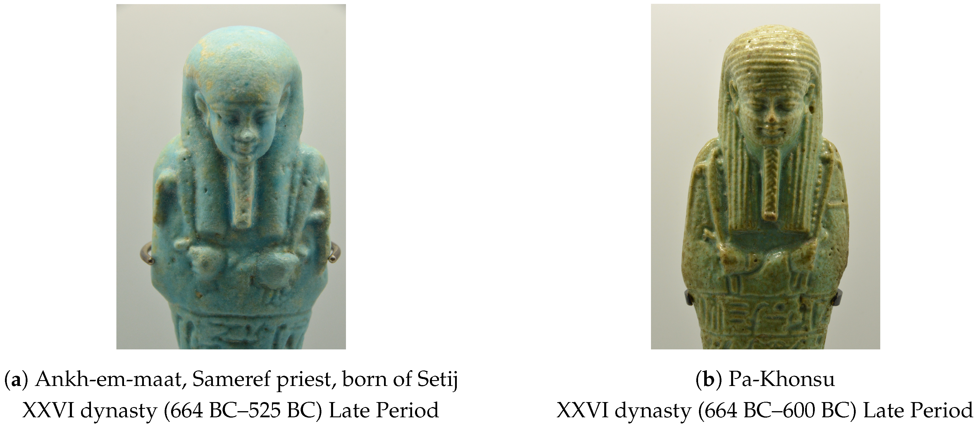
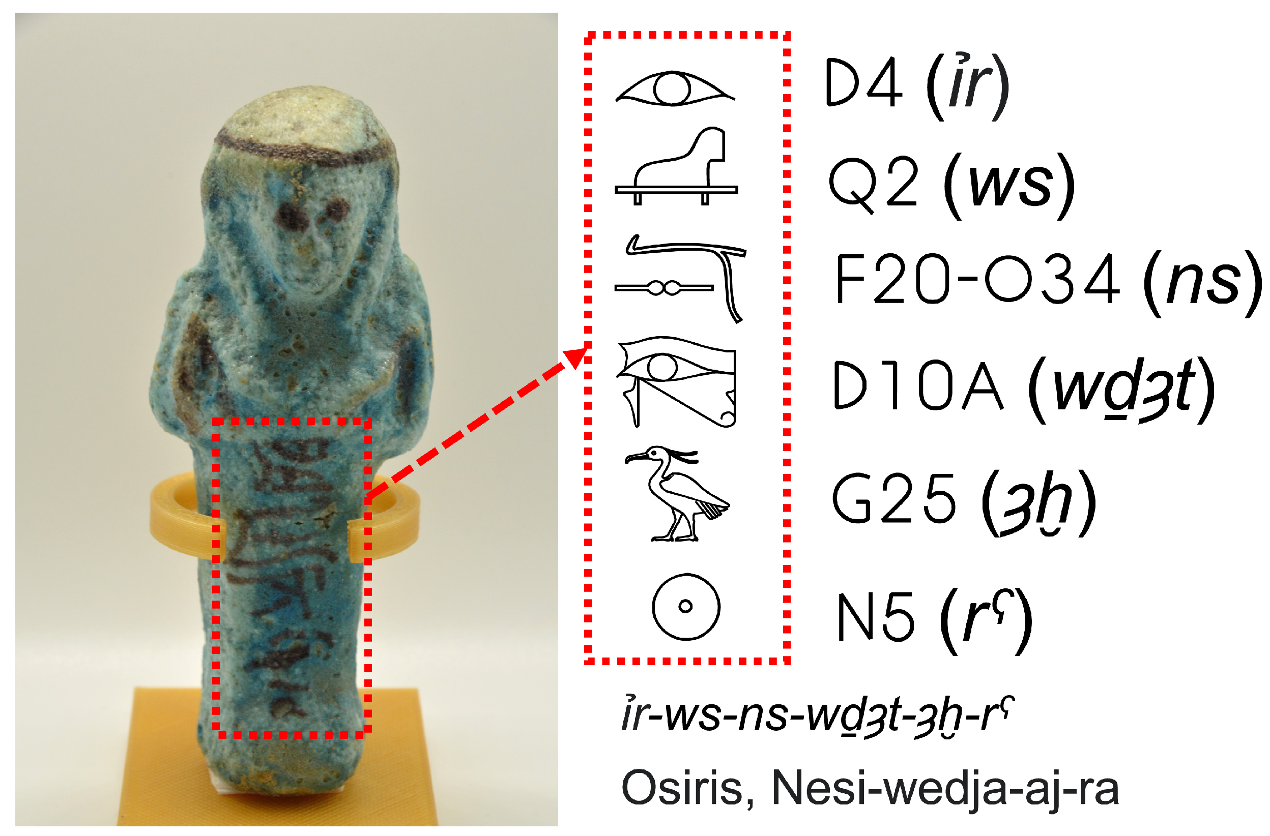
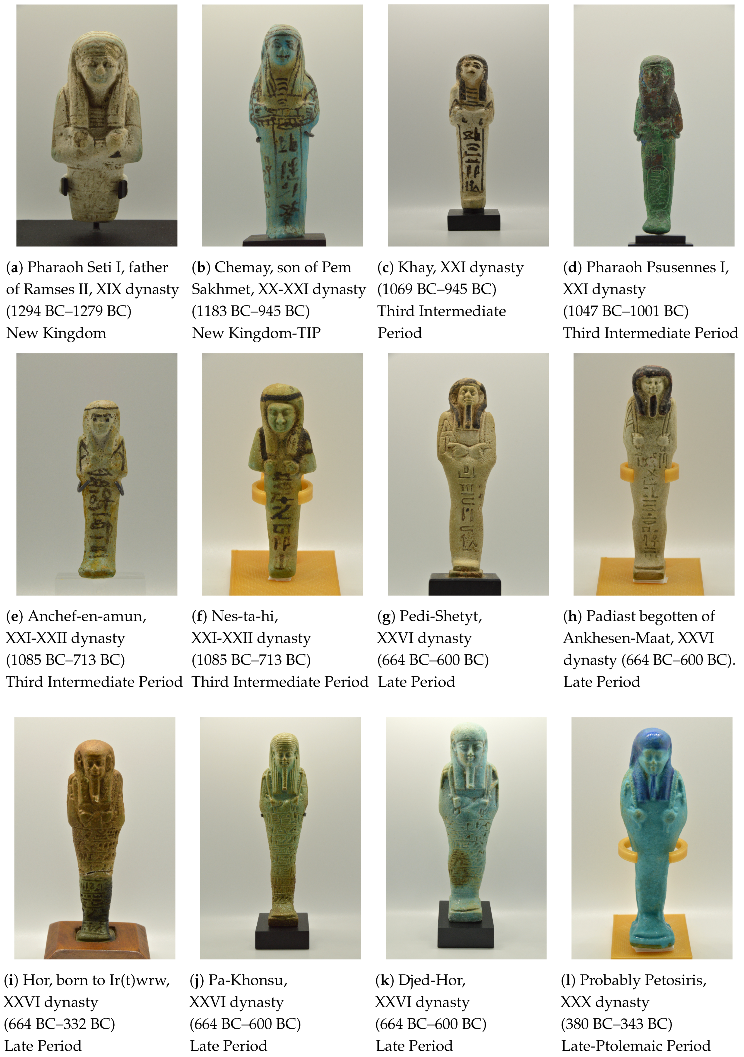
3.1. The Classification of Shabtis

Shabtis were created in different styles and materials. They were initially produced in small amounts and manually decorated. Although some examples have been found from the XIIth dynasty, during the Middle Kingdom (2055 BC–1650 BC), it was during the New Kingdom (1550 BC–1069 BC) when they became common and a lot of people were buried with a different number of servants, which the real function of a shabti was. During the Third Intermediate Period (1069 BC–664 BC), the shabtis were not as refined as during the New Kingdom, although most of them were manually decorated and painted, as shown in Figure 2. Many shabtis have different kinds of inscriptions showing the name of the deceased.
The style of the shabtis was different depending on the period. Figure 3 shows different shabtis, most of them used during training. A hand-written shabti of the biblical pharaoh Seti I (Figure 3a), father of Ramses II and produced during the XIX dynasty (1294 BC–1279 BC) of the New Kingdom, is quite different from a bronze shabti of the pharaoh Psusennes I (Figure 3d), produced during the XXI dynasty (1047 BC–1001 BC) of the Third Intermediate Period (TIP); or a molded green faience shabti of Pa-Khonsu (Figure 3j) produced during the XXVI dynasty (664 BC–350 BC) of the Late Period; or a bi-chrome blue shabti probably of Petosiris (Figure 3l), produced during the XXX dynasty (380 BC–343 BC) of the Late and Early Ptolemaic Period. During different Egyptian periods, there were changes in materials, hieroglyphs inscription formulas, wigs, the working instruments or even the beard. Seti I, being a pharaoh, is not represented with the Osiris beard. However, Pa-Khonsu used this attribute because, at his time, shabtis used beards. During a particular period of time, it is possible to find similar-style shabtis used for several people. However, there is usually a difference, since they were normally manually produced and adapted to different people’s tastes. The shabtis of Pe-di-setyt (Figure 3g) and the Padiast (Figure 3h) are quite similar because they were probably produced during the same period of time, XXVI dynasty (664 BC–600 BC), and probably in a nearby location, but it is possible to find significant differences that are also identified by the neural networks. The shabtis of Anchef-en-amun (Figure 3e) and Nes-ta-hi (Figure 3f) were probably produced in the same Egyptian period but, as in the previous example, there are observable differences that can be learnt by a CNN.

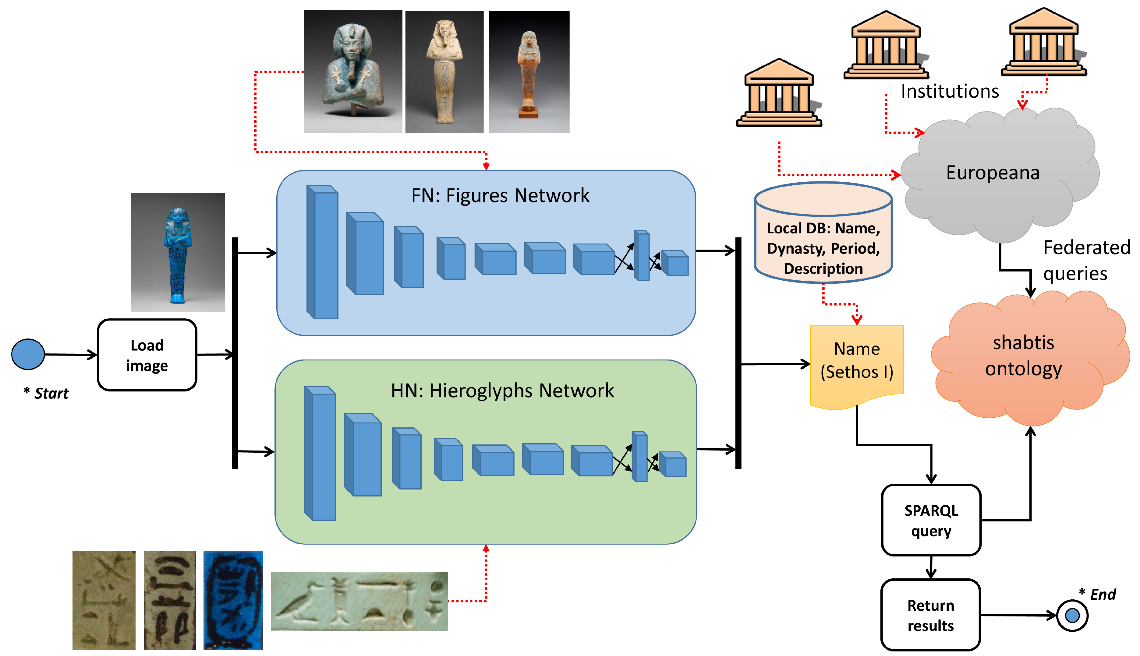
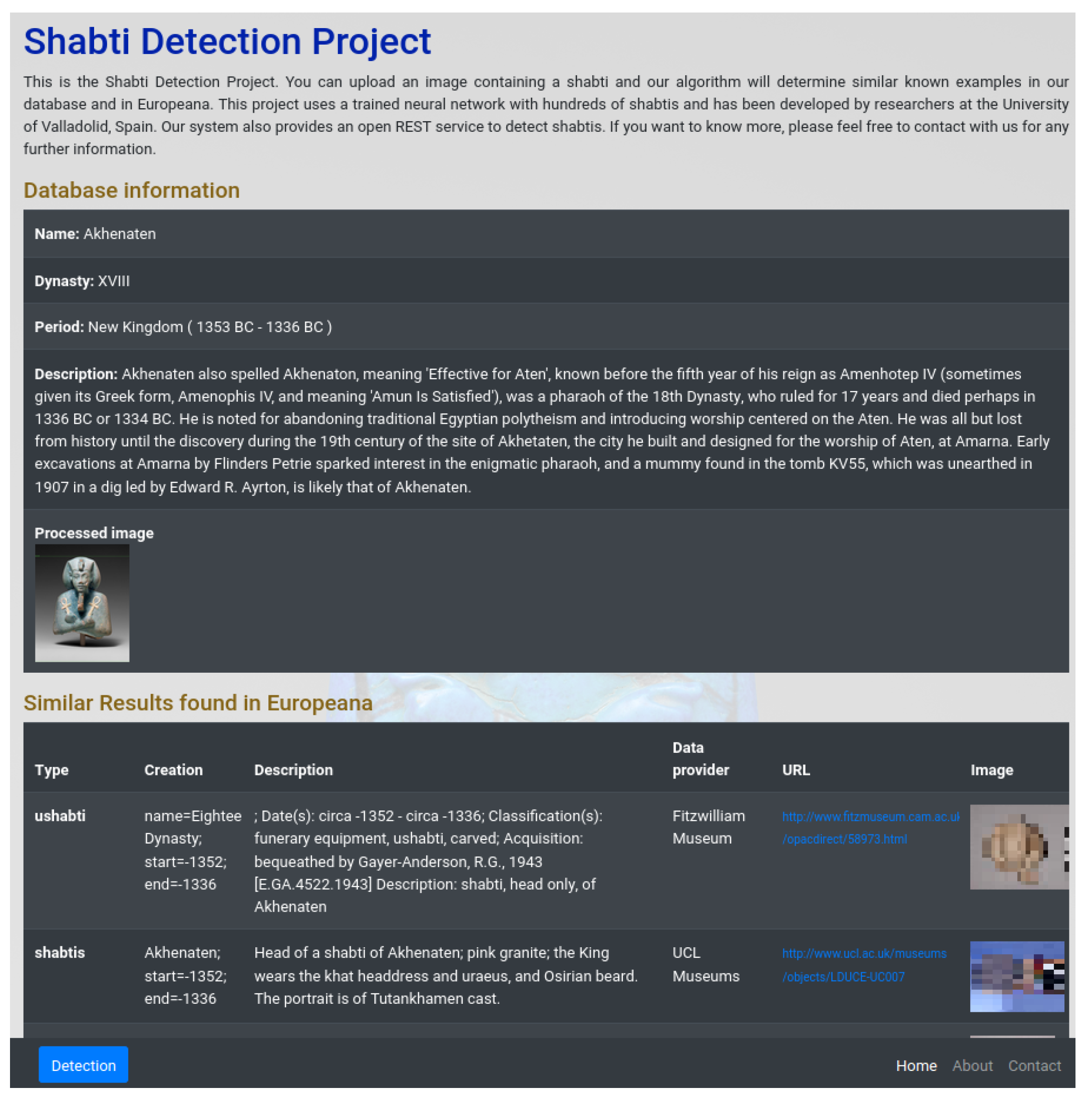
3.2. The System to Detect Shabtis

The system is composed by two different parts. The first part is responsible for the detection of the shabti using computer vision. The second part obtains data from Europeana when a name has been detected. Figure 4 shows the schema of the system.
Although a unique network could be trained to detect both kinds of object at the same time; in our work, we have preferred to decouple this process, so it is easier to make modifications or perform new trainings in each module separately. Moreover, the results are improved when two networks are responsible for detecting different elements. In our system, a first network, named Figures Network (FN), detects shabtis by their complete figure. A second network, named Hieroglyphs Network (HN), only detects Egyptian names written in hieroglyphs.
There are two main reasons for using the concept of two different networks. On the one hand, some shabtis have clear hieroglyphs that are well repeated in different examples for a concrete person. It is important to note that, although it is possible to find two similar shabtis of two different persons with the same name, it is uncommon. If the style of two shabtis is very similar and the name is the same, it is likely to be the same owner. Moreover, some shabtis are broken and only some fragments have been found. In this case, the detection of the name in hieroglyphs is essential because a comparison between the figure and other complete examples is not possible. On the other hand, the inscription of some shabtis is illegible. These cases require the detection of the complete figure. In addition, some shabtis do not have an inscription or they do not have it on its front, such as the examples of Petosiris (see Figure 3l) or Hekaemsaf. In these situations, the hieroglyphs detection makes no sense and the detection of the complete figure is required. One question that arises at this point is whether it is possible to detect the owner of a shabti by its figure or not. The answer is that many times it is. People who work in cataloguing shabtis are used to identifying the owner of a shabti in many situations just by looking at the figure and without reading the hieroglyphs. Some examples do not even have inscriptions, but are likely to be from the same owner, as shown in Figure 5. Going back to a previous example, the shabti of Seti I (see Figure 3a) is practically illegible because its text cannot be read well. Some cartouches with the name of the pharaoh can be seen, but it is impossible to read them correctly. However, it is clearly a shabti of Seti I of an excellent manufacture not seen in any of the other shabtis of Figure 3.
A database with 1111 images and 151 different shabti owners has been created for the FN. Before training the Yolo network, a process has been carried out to extract the saliency of each image. This process automates the manual labelling of shabtis, which requires an enormous amount of time. The saliency corresponds to what stands out in a photo, focusing on the most important regions. As an example, the saliency of the shabti of Seti I (Figure 6a) is shown in Figure 6b.
The saliency algorithm is based on the model presented by Montabone and Soto [41], where the authors presented VSF (Visual Saliency Features), a method to extract features based on a biologically inspired attention system [42,43] and providing fine grained feature maps and much more defined borders than other previous methods such as VOCUS. The VSF method implements the same filter windows as those used in VOCUS, which converts the original color image into grayscale and creates a Gaussian image pyramid, applying a 3 × 3 Gaussian filter and a scaling down factor four times consecutively. Finally, the system only takes into account the information present in the smallest scales. However, VSF uses an integral image on the original scale to obtain high quality features. Although VSF has been widely used in human detection extraction, it has produced excellent results in our problem, and less than 10% of the labels of the shabtis have been manually updated.
The importance of saliency consists in the need for some DNN algorithms, such as YOLO, to know the limits of the objects that have to be recognized. In Figure 6c, the limits of the shabti of Seti I are obtained, detecting the first/last active pixels in the saliency map. The center of this region and the width and height are the parameters used with the image to train the network.
In addition to the figures database, the HN has been trained with the names of some of the shabtis of the main database, concretely 201 names for 60 different shabtis. These names have been manually labelled, since it is necessary to read the hieroglyphs and filter the concrete names. Some parts of the inscriptions refer to the name of the parents, the titles of the deceased (see Figure 7), religious expressions (see Figure 8) or even Chapter VI of the Book of the Dead in shabtis with several lines of text. Figure 9 shows the manual annotation of some of the names.
The names found on two shabtis of the same person tend to be very similar, either because they were created through a mold, or because they were written in the same way, using the same hieroglyphics in the same position. In some cases, the name may appear in a different form or in different material on several groups of shabtis from the same tomb. However, the different cases of names have been included during the training.
The two networks, FN and HN, have been implemented using YOLOv3. Two important aspects of YOLO are necessary for our project. One is a detector, which is necessary since our problem is an identification problem, and the other is the feature of returning the bounding boxes to compare the results obtained by FN and HN. In this way, it is possible to discern whether a name in hieroglyphics detected by the HN is within a shabti detected by the FN. Unlike other methods that use pipelines for detection or classification, YOLO [31] uses a single neural network. YOLO receives an image as input and returns a bounding box vector and the prediction percentage of the corresponding detected categories as output. The input image is divided into a grid of S · S cells. For each object present in the image, the cell in which the center of the object is located is responsible for its prediction. Each grid cell predicts the bounding boxes, B, and the class probabilities, C. The output of the network consists of bounding boxes as well as class probabilities. The prediction of each bounding box has 5 components: ( x , y , w , h , c o n f i d e n c e ) . The coordinates ( x , y ) represent the center of the box, relative to the location of the grid cell; while ( w , h ) are the weight and height of the box relative to the size of the image. The confidence shows the certitude that an object of these dimensions is present at that position. In addition, in each cell, there are probabilities corresponding to each of the possible classes. YOLO uses a single CNN network with different convolutional, max pooling and full-connected layers. The convolutional layers extract features, called feature maps, and the pooling layers distill features down to the most salient elements. Several consecutive pairs of convolutional and pooling layers are aimed at first extracting simple characteristics, such as lines or vertices, to more complex characteristics, as in our case would be the shape and outstanding attributes of a shabti. It also uses sequences of 1 x 1 reduction layers and 3 × 3 convolutional layers inspired by the GoogLeNet model (Inception) [44,45] and the Network in Network (NiN) model to reduce the number of features before costly parallel blocks.
Some parameters established in both networks (FN and HN) have been: batch = 64, subdivisions = 16, width = 416, height = 416, channels = 3, momentum = 0.9, decay = 0.0005, angle = 0, saturation = 1.5, exposure = 1.5, hue = 0.1, learning rate = 0.001. YOLOv3 is composed of 75 convolutional layers, 23 shortcut layers after CNN-layers to propagate gradients further and allow efficient training, 4 route layers to merge precedent layers into one layer, 2 up-sample layers used for deconvolution and 3 Yolo layers responsible for calculating the loss at three different scales.
A procedure for identifying a shabti using the two networks has been established. The procedure is the following:
  • An input image is introduced in the two YOLO networks.
  • If the FN model returns some detections ( F N 1 , F N 2 ,..., F N x ), the class with the highest confidence, F N i , is selected after applying non-maxima suppression to suppress weak, overlapping bounding boxes.
  • If the HN model returns some detections ( H N 1 , H N 2 ,..., H N y ), the class with the highest confidence, H N j , is selected after applying non-maxima suppression to suppress weak, overlapping bounding boxes.
  • If both models have returned detections, F N i is selected when c o n f i d e n c e ( F N i ) > c o n f i d e n c e ( H N j ) , and H N j otherwise. If the bounding box H N j is not inside the bounding box F N i , the non-selected class is also shown to the user as another possibility whenever the class is different.
  • If only the FN model has returned detections, F N x is selected.
  • If only the HN model has returned detections, H N y is selected.
  • Local data and data retrieved from Europeana are shown for the selected class.
In CNNs, the square average error is often used as a loss function. However, YOLOv3 detects the bounding boxes and, hence, the loss function is different. This concept is necessary for our project when detecting more than one shabti at the same time. Since two networks have been used (FN and HN), when both of them detect a shabti, it is necessary to check whether the HN bounding box is inside the FN bounding box or not. If not, these hieroglyphs are not part of the shabti detected by the FN model. Specifically, this function is the following:
e = λ c o o r d i = 0 S 2 j = 0 B 𝟙 i j o b j x i x i ^ 2 + y i y i ^ 2 + λ c o o r d i = 0 S 2 j = 0 B 𝟙 i j o b j w i w i ^ 2 + h i h i ^ 2 + i = 0 S 2 j = 0 B 𝟙 i j o b j C i C i ^ 2 + λ n o o b j i = 0 S 2 j = 0 B 𝟙 i j n o o b j C i C i ^ 2 + i = 0 S 2 𝟙 i o b j c c l a s s e s p i ( c ) p i ^ ( c ) 2
where the first term evaluates, for each grid S · S and each bounding box B detected in each grid, the error of the central position ( x , y ) of the bounding box of some found object compared with the real value that the bounding box should have. 𝟙 i j o b j is 1 if an object is present in grid cell i and the predictor in bounding box j is responsible for that prediction. The second term uses a similar idea but, instead of checking the central point of the bounding box, what is checked is the size of a bounding box, height w and width h, compared with the real object used during the training. Regarding the third term, the concept is the same as in the previous terms, but the confidence ( C i ) that the detected bounding box really corresponds to an object ( C i ^ ) is evaluated. This term also penalized incorrect detections. The λ parameters are used to balance the different parts of the loss function. The fourth term is actually responsible for the classification problem, inferring whether an object located on the grid i is of the class we are looking for. The indicator function, 𝟙 i o b j is 1 if an object is present in a cell i, and 0 otherwise. This function seems similar to a quadratic error used in a classification problem except for 𝟙 i n o o b j . This indicator is used to avoid penalizing the error when no object is present in the cell. In YOLO, as in other neural networks, the gradient descent optimization algorithm is used to minimize the error function to achieve an overall minimum.
YOLO2 [32] introduced several modifications to YOLO, such as:
  • Batch normalization, to help regularize the model and reduce overfitting.
  • High resolution images, passing from small input images of 224 × 224 to 448 × 448.
  • Anchor boxes, to predict more bounding boxes per image.
  • Fine-grained features, which helps to locate small objects while being efficient for large objects.
  • Multi-scale training, randomly changing the image dimensions during training to detect small objects. The size is increased from a minimum of 320 × 320 to a maximum of 608 × 608.
  • Modifications to the internal network, using a new classification model as a backbone classifier.
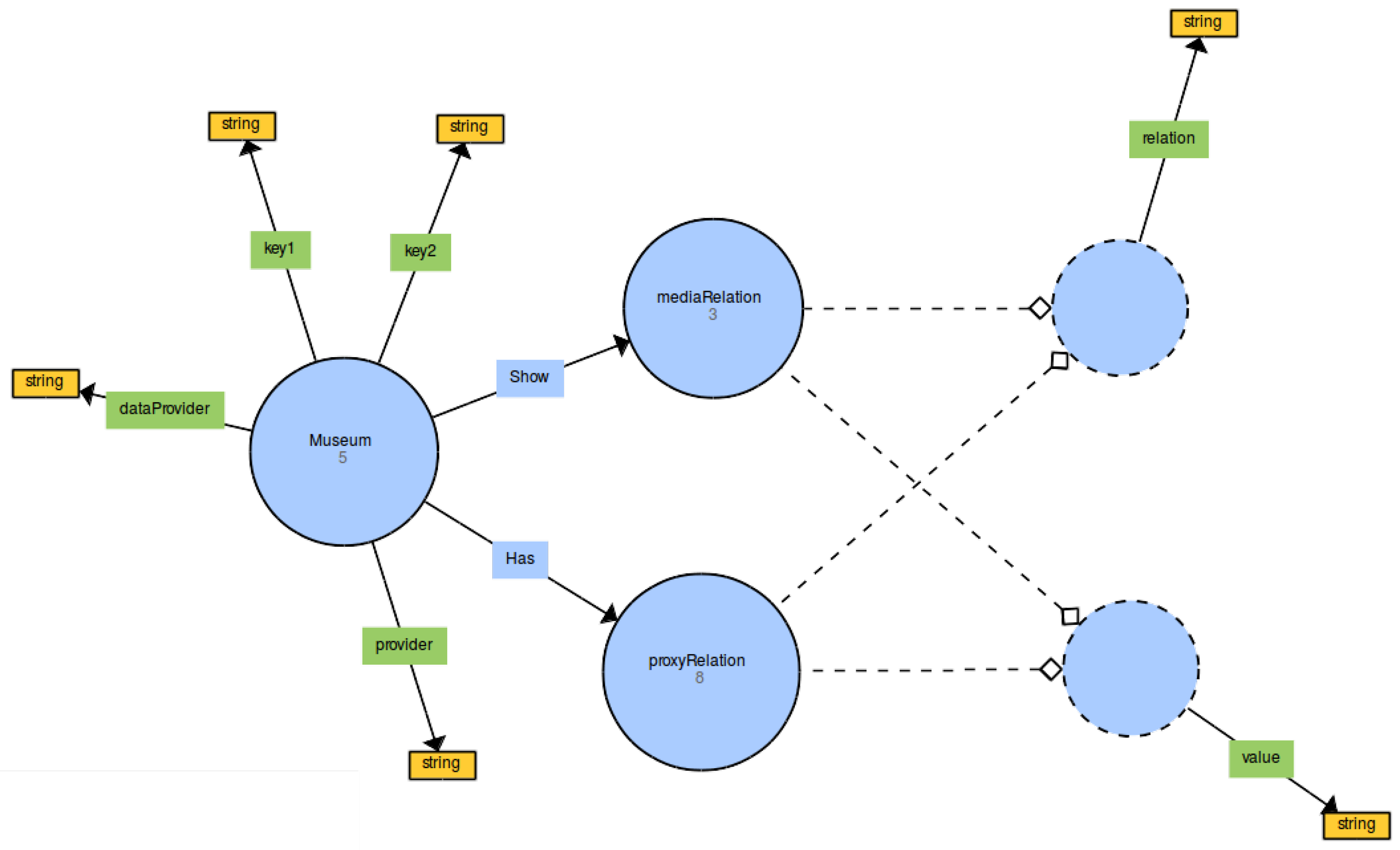
In addition, YOLO3 [30] has included some modifications, called incremental improvements, making some changes in the bounding box and category predictions together with prediction across scales. The prediction across the scales extracts features from each scale and uses a method based on feature pyramid networks.

3.3. New Ontology

An ontology is a specification of a conceptualization [35,36], which defines and classifies concepts, entities, and the relationships between them. An ontology integrates entities, such as classes or dependencies, and formal axioms to limit the interpretation and well-formed use of them. Classes provide a mechanism of abstraction to group resources with similar characteristics. Two class identifiers have been predefined in the OWL semantic Web language: the Thing and No Thing classes. The Thing extension is the set of all individuals, while No Thing it is the empty set. Each OWL class is a subclass of Thing [37]. The individuals represented in the extension of the class are the instances of the class. When a class is defined as a subclass, their individuals are a subset of the individuals contained in the parent class.
Two main categories of properties are defined in OWL: object properties, which link individuals; and data type properties, which assign individuals to data values. On the other hand, range and domain are axioms used during the inference process, which is the process of deduction that allows knowledge to be obtained from known data and existing relations in the ontology. A range axiom assigns a property to a data range, specifying the range of the data values. A domain axiom assigns a property to a class description, specifying the extension of the indicated class.
A problem that was found during our research is that obtaining data from multiple cultural institutions via Europeana is not unified, since every institution has used their concrete terms to catalogue their collections. When a new application is created, a different query has to be implemented to access each institution, i.e., University College of London (UCL) or Israel Museum. Moreover, the keys that were used in each query were different. Each institution has the information to search in a different concept, i.e., the name of the shabti. A new ontology was designed to integrate different institutions and thus be able to obtain data with just one query. This ontology was also designed to specify the keys that had to be used in the query.
There are three general subclasses of Thing: Museum, proxyRelation and mediaRelation (see Figure 10). The extension of the class Museum refers to cultural institutions, such as the UCL, Fitzwilliam Museum or Israel Museum. Europeana includes Cultural Heritage Objects (CHO) that are associated to concrete proxies. The class proxyRelation specifies which URIs are significant for a museum. Simultaneously, the class mediaRelation specifies the possible media relations of a museum, i.e., photos of the object.
The class Museum has different data properties. key1 and key2 specify the URIs used to search in that museum. For example, key1 = http://purl.org/dc/elements/1.1/type specifies that the concept type of http://purl.org/dc/elements/1.1 will be used to search for the term “shabti”. The property dataProvider specifies the name of the institution, i.e., “UCL Museums”. A museum is linked to a general provider and the property provider is used for that purpose, i.e., “AthenaPlus”. This property could be omitted, but the query would not work due to a time out. Data has to be filtered to work in a reasonable time. All the used data properties are of type xsd:string.
The classes proxyRelation and mediaRelation have two data properties: relation and value. relation specifies the URI used to link the concept indicated by value with the proxy of the CHO (proxyRelation) or just the CHO (mediaRelation). For example, in a proxyRelation, it is possible to specify relation = http://purl.org/dc/elements/1.1/title and value = “title”. The inference will search for a relation of the proxy using the URI specified by relation and the result will be named “title”. These two data properties are xsd:string.
There are two object properties: Has and Show. The domain of Has is Museum and the range is proxyRelation. The domain of Show is Museum and the range is mediaRelation. These object properties link the cultural institutions with their respective relations.
Several individuals have been created, one for each cultural institution. There are different relations and each cultural institution can share some of them. As an example, UCL is defined by next data properties (Table 1) and object properties (Table 2).
The ontology has been implemented using Protégé 5.5 [46] and an Apache Jena Fuseki server [47] has been deployed to support the ontology and give an endpoint for the application. To connect Europeana’s SPARQL remote endpoint, federated queries have been used [48].

4. Experiments and Results Discussion

An initial comparison between YOLO v3 and different techniques of object detection were evaluated. They included methods based on feature extraction such as SIFT [27], SURF [28] or ORB [29]. The matchers used with SIFT, SURF and ORB were respectively FLANN, BF, and Hamming KNN [49]. YOLO was chosen because the results were better when faced with new images (70.06% vs. 61.16% SIFT, 17.85% SURF and 56.70% ORB) and, in addition, its processing time was much faster (0.15 s vs. 16.75 s SIFT, 1.24 s SURF and 1.61 s ORB). Moreover, when the training set grows, SIFT, SURF or ORB processing times also increase because these methods must match the input image descriptors with all the image descriptors in the database to get the closest match. YOLO has no such problem, since once the model is trained, its runtime remains stable regardless of the size of the dataset. However, YOLO v3 needs a heavy initial training.
One problem with the shabtis is that there are not many known shabtis for each owner. In some cases, it is possible to find more than 50 examples, such as Seti I or Pinudjem I, but for most of them, less than 10 examples are usually found in museums or private collections. In some cases, such as Pa-khonsu, only one example is known. To avoid overfitting of the network because of this particular situation, data augmentation is carried out during the training, creating random images obtained by changing the parameters of the original images, such as the saturation, exposure or hue.
The list of shabti owners used for the training of the FN is shown in Table 3. Some people had the same name, although it could be written in a different manner, as Henut-tawy and Henut-tawy (Queen), who were two different persons. The reason is because there were different hieroglyphs with the same phonetic sound and even transliteration in our language. Other owners had completely different shabtis produced in several materials. For these cases, the category has been decoupled to make the network split the objects more accurately. Some examples are the famous Tutankhamen (Faience and Wood), Amenophis III (Limestone and Wood), or Ramses III (Alabaster, Stone and Wood). In total, there are 158 categories for 151 different shabti owners. 64 out of these 158 categories were used to train the HN, since the names of hieroglyphs could only be read for images of 64 classes. 815 images have been used, respectively, for the FN and HN trainings. 354 images have been used for the tests.
The YOLO FN training took 398 h (316,000 iterations), while the HN training took 148 h (128,000 iterations) in a i9-9900K/32 Gb with a GPU RTX2080-TI. Figure 11 shows the loss function during the first iterations of the FN/HN training, taking a value lower than 1.0, starting from the iteration 400. The rest of the trainings progressively decrease the loss value to less than 0.01 in the final iterations. The success of the models against the test dataset is shown in Figure 12 for the first 40,000 iterations. This success represents the percentage of correct detections of the 354 test images.
The main objective of the HN network is to detect shabtis by name, so even though there are less training data and fewer classes in the network, it allows to filter those classes in a more unequivocal way. However, many times the names are not clear or have not been represented, so the combination with the FN network is necessary. The combination of FN and HN improves the success of both networks, achieving 70.06% of correct detections in the complete test dataset (354 images), against FN (66.10% of 354 images) and HN (66.38%, considering that in this case the test set was composed of 200 images, which is smaller because the number of classes was lower). However, some shabtis were not detected as positive or negative. Considering only positive and negative detections the results are: 82.10% of success for the FN model that has detected 285 shabtis (positive + negative), 78.07% of success for the HN model that has detected 153 shabtis (positive + negative) and 82.39% of success for the FN + HN model that has detected 301 shabtis (positive + negative). These results clearly show that the combination of both models significantly improves the positive detections.
A Precision-Recall (PR) curve has been obtained to evaluate the FN, HN and FN + HN models. The Average Precision (AP) has been computed by integrating the curve, therefore computing the Area Under the Curve (AUC). Figure 13a shows the PR curve for the FN network with an A P = 0.73. Figure 13b shows the PR curve for the HN network with an A P = 0.61. Figure 13c shows the PR curve for the FN + HN model with an A P = 0.79. As previously explained, the combination of both models, FN and HN, improves the model, since the system is able to detect the shabtis either by their shape or by their name.
Regardless of whether the system returns the proper owner or not, another important issue is giving the right dynasty and period. Although a shabti could be wrong, it is important to return a similar shabti of the same dynasty or period. The FN + HN model returns the right dynasty in 74.86% of cases and the right period in 81.36% of cases. Considering only the 301 detected shabtis of the FN + HN model, the right dynasty is given in 88.04% of cases and the right period in 95.68% of cases. A confusion matrix of the dynasty and period detection is shown in Table 4 and Table 5 respectively.
With regard to the confusion matrix of the dynasties, most of the errors are situated close to the diagonal. This means that our approach is able to identify that the shabti was produced near that dynasty or period of time. For example, some shabtis of the XXI dynasty were detected between the XXth and the XXII dynasties, but these dynasties happen in a short slot of time according to Egyptian history. In some cases, shabtis of different dynasties, far distant in time, were wrongly detected. For example, shabtis of the XVIII dynasty are detected in the XXVI-XXX dynasty. This happens because some examples of the previous dynasty were reproduced in a very similar style in the next dynasties.
Concerning the confusion matrix of the periods, it is important to note that there were shabtis detected on the limit between periods. As an example, the XX dynasty corresponds to the New Kingdom while the XXI dynasty corresponds to the Third Intermediate Period. In these two dynasties, which are very close together, the style of some shabtis were very similar. However, in most cases, the success was 95.68% of correct period identification, as presented before.
Although our problem is different from others published, a comparison with similar archaeological problems, such as the ancient coin or pottery sherds classification, can be established. Aslan et al. [18] obtained a classification accuracy of 73.6% detecting 60 types of Roman coins; Zambanini and Kampel [17] obtained a classification accuracy of 71.4% also detecting 60 types of Roman coins; and Anwar et al. [22] showed an accuracy depending on the class (i.e., 68.15% for coins with a quadriga or 79.28% with a curule) in CoinNet. Regarding the classification of archaeological pottery sherds, Makridis and Daras [24] obtained an accuracy of 78.26% detecting 8 classes of ceramic. Llamas et al. [23] obtained a better accuracy detecting architectural heritage images (94.59%), but there were only 10 types of architectural elements. In our problem, the number of classes is much larger, obtaining an accuracy of 70.06% detecting 158 categories.
As previously explained, when a shabti has been identified, our system shows some local data previously collected (name, dynasty, period, description) and connects the data to the cultural institutions that have similar shabtis by means of our ontology and Europeana. This connection returns similar examples of the shabti. An example of a SPARQL query to obtain shabtis for Akhenaten is shown in Listing 1, where the syntax word SERVICE links our ontology with Europeana. The search is carried out with “habti” instead of “Shabti” because the term can be found with “Ushabti” or “Shabti” and it is case sensitive.
Some of the results returned by this query are shown in Table 6, where it is possible to see data from different institutions: UCL, Fitzwilliam Museum or Israel Museum. There are two results from the UCL and some properties have different values, i.e., type, which has the value “funerary equipment” but also “ushabti” for Fitzwilliam Museum. The Israel Museum has two identifiers for each shabti. Unlike a structured database, semantic searches are open to this type of possibility, defining certain properties for an individual that may be repeated or even not present in another similar individual in the same class.
A complete deployable application (see Figure 14) using Docker [50] is available on the Internet at the URL: https://drive.google.com/drive/folders/1nRn4jAz2RzTD_AisSJbhv0EptJthgLL_. This application integrates the full process and returns data from our local database and known examples from Europeana.
Listing 1. Query to obtain shabtis of Akhenaten
PREFIX shabt i s : <http://www.amenofis.com/shabtis.owl#>
PREFIX dc : <http://purl.org/dc/elements/1.1/>
PREFIX dc_e : <http://purl.org/dc/terms/>
PREFIX edm: <http://www.europeana.eu/schemas/edm/>
PREFIX rdf : <http://www.w3.org/1999/02/22–rdf–syntax–ns#>
PREFIX ore : <http://www.openarchives.org/ore/terms/>
PREFIX skos : <http://www.w3.org/2004/02/skos/core#>
PREFIX rdf s : <http://www.w3.org/2000/01/rdf–schema#>
SELECT DISTINCT
(GROUP_CONCAT(DISTINCT CONCAT( ? value , " : " , s t r ( ? val ) ) ;
SEPARATOR=" ; ; ; " ) AS ? r e l a t ionVa lue s )
(GROUP_CONCAT(DISTINCT CONCAT( ? sValue , " : " , s t r ( ? sVal ) ) ;
SEPARATOR=" ; ; ; " ) AS ? showValues )
?ProvidedCHO ? dataProvider ? provider
WHERE
{
?museum shabt i s : provider ? provider .
?museum shabt i s : dataProvider ? dataProvider .
?museum shabt i s : key1 ? key1 .
BIND( IRI ( ? key1 ) AS ?k1 ) .
?museum shabt i s : key2 ? key2 .
BIND( IRI ( ? key2 ) AS ?k2 ) .
?museum shabt i s :Has ? pRelat ion .
? pRelat ion shabt i s : r e l a t i o n ? r e l a t i o n .
BIND( IRI ( ? r e l a t i o n ) AS ? r e l ) .
? pRelat ion shabt i s : value ? value .
?museum shabt i s : Show ? sRe l a t ion .
? sRe l a t ion shabt i s : r e l a t i o n ? showRelation .
BIND( IRI ( ? showRelation ) AS ? sRel ) .
? sRe l a t ion shabt i s : value ? sValue .
SERVICE <http://sparql.europeana.eu>
{
?ProvidedCHO edm: dataProvider ? dataProvider .
?ProvidedCHO edm: provider ? provider .
?proxy ore : proxyIn ?ProvidedCHO.
?proxy ?k1 ?v1 .
?proxy ?k2 ?v2 .
?proxy ? r e l ? val .
?ProvidedCHO ? sRel ? sVal .
FILTER (CONTAINS( ? v1 , " habt i " ) && CONTAINS( ? v2 , "Akhenaten " ) ) .
} }
GROUP BY ?ProvidedCHO ? dataProvider ? provider

5. Conclusions

This paper presents a novel use of computer vision for Egyptology. Ancient Egyptians were buried with hundreds of small servants, called shabtis. These statuettes helped them in the afterlife. A lot of museums and private collections around the world are potential users of our approach, since it can help them to identify their pieces. We have to thank Glenn Janes, global expert with several published books referenced by the main museums, for his help in providing us with examples to train our networks.
Although computer vision has been applied to the classification of ancient coins and archaeological pottery, no other work has been published regarding the classification and identification of shabtis. Using the latest technology, the YOLO v3 neural network, our work demonstrates that it produces better results identifying 158 different categories than other previous techniques, such as SIFT. In our problem, the detection has been carried out using two different models, one for the detection of the figure itself, and another for the detection of the name in hieroglyphics. Both networks are simultaneously processed and increase the performance of the system, detecting properly more than 70% of 354 shabtis in our test dataset. In the case of detected shabtis, the results are over 82% and the dynasty classification is over 88%, while the period classification is near 96%.
The CNN used can work with up to 1000 classes offering good results. However, in our experience, their behavior worsens when the number of classes is too high. For this reason, if our system grows much further, different networks could be used for groups of classes, so that the winner among different networks would be the one that offers more confidence, similar to what is done between the FN and HN network.
In addition to shabti identification, a semantic connection with Europeana has been established. When a shabti is identified, some data are provided by a local database, while a search for shabtis of the same person is carried out in the different institutions linked to the Europeana semantic system to offer the user known examples of that concrete shabti. A web application implementing the full process has been deployed.
Future works will consist in integrating more data from different museums and the use of our system with other archaeological items. Other archaeological items, such as Egyptian sculpture, are also written in hieroglyphs and the use of two neural networks is also replicable.

Author Contributions

J.D.D. contributed to the entire work, creating the dataset, designing the experiments, analyzing the results and preparing the paper. J.G.-G.-B. and E.Z. contributed to the work as scientific directors, monitoring the work progress, analyzing the results and preparing the paper. All authors have read and agreed to the published version of the manuscript.

Funding

The present research has been partially financed by “Programa Retos Investigación del Ministerio de Ciencia, Innovación y Universidades (Ref. RTI2018-096652-B-I00)” and by “Programa de Apoyo a Proyectos de Investigación de la Junta de Castilla y León (Ref. VA233P18)”, co-financed by FEDER funds.

Acknowledgments

We have to thank Glenn Janes, global expert with several published books referenced by different museums, for his help in providing us with examples to train our networks.

Conflicts of Interest

The authors declare that there is no conflict of interest regarding the publication of this manuscript.

References

  1. Quibell, J. Note on a tomb found at Tell er Roba. In Annales du Service des Antiquités de l’Égypte; Conseil Suprême des Antiquités Égyptiennes: Cairo, Egypt, 1902; Volume 3, pp. 245–249. [Google Scholar]
  2. Schneider, H.D. Shabtis: An Introduction to the History of Ancient Egyptian Funerary Statuettes with a Catalogue of the Collection of Shabtis in the National Museum of Antiquities at Leiden: Collections of the National Museum of Antiquities at Leiden; Rijksmuseum van Oudheden: Leiden, The Netherlands, 1977. [Google Scholar]
  3. Stewart, H.M. Egyptian Shabtis; Osprey Publishing: Oxford, UK, 1995; Volume 23. [Google Scholar]
  4. Petrie, S.W.M.F. Shabtis: Illustrated by the Egyptian Collection in University College, London; Aris & Phillips: London, UK, 1974. [Google Scholar]
  5. Janes, G.; Bangbala, T. Shabtis, A Private View: Ancient Egyptian Funerary Statuettes in European Private Collections; Cybèle: Paris, France, 2002. [Google Scholar]
  6. Aubert, J.F.; Aubert, L. Statuettes égyptiennes: Chaouabtis, Ouchebtis; Librairie d’Amérique et d’Orient: Paris, France, 1974. [Google Scholar]
  7. de Araújo, L.M. Estatuetas Funerárias Egípcias da XXI Dinastia; Fundação Calouste Gulbenkian: Lisboa, Portugal, 2003. [Google Scholar]
  8. Newberry, P.E. Funerary Statuettes and Model Sarcophagi; Catalogue général des Antiquités Égyptiennes du Musée du Caire; Institut français d’archéologie orientale, Service des Antiquités de l’Égypte: Cairo, Egypt, 1930. [Google Scholar]
  9. Bovot, J.L. Les Serviteurs Funéraires Royaux et Princiers de L’ancienne Egypte; Réunion des Musées Nationaux: Paris, France, 2003. [Google Scholar]
  10. Brodbeck, A.; Schlogl, H. Agyptische Totenfiguren aus Offentlichen und Privaten Sammlungen der Schweiz; OBO SA; Universitätsverlag Freiburg Schweiz, Vandenhoeck und Ruprecht Göttingen: Fribourg, Switzerland, 1990; Volume 7. [Google Scholar]
  11. Janes, G. The Shabti Collections: West Park Museum, Macclesfield; Olicar House Publications: Cheshire, UK, 2010. [Google Scholar]
  12. Janes, G.; Gallery, W.M.A. The Shabti Collections. 2. Warrington Museum & Art Gallery; Olicar House Publications: Cheshire, UK, 2011. [Google Scholar]
  13. Janes, G.; Moore, A. The Shabti Collections: Rochdale Arts & Heritage Service; Olicar House Publications: Cheshire, UK, 2011. [Google Scholar]
  14. Janes, G.; Cavanagh, K. The Shabti Collections: Stockport Museums; Olicar House Publications: Cheshire, UK, 2012. [Google Scholar]
  15. Manchester University Museum; Janes, G. The Shabti Collections: A Selection from Manchester Museum; Olicar House Publications: Cheshire, UK, 2012. [Google Scholar]
  16. World Museum Liverpool; Janes, G. The Shabti Collections: A Selection from World Museum, Liverpool; Olicar House Publications: Cheshire, UK, 2016. [Google Scholar]
  17. Zambanini, S.; Kampel, M. Coarse-to-fine correspondence search for classifying ancient coins. In Proceedings of the Asian Conference on Computer Vision, Daejeon, Korea, 5–9 November 2012; Springer: Berlin, Germany, 2012; pp. 25–36. [Google Scholar]
  18. Aslan, S.; Vascon, S.; Pelillo, M. Ancient coin classification using graph transduction games. In Proceedings of the 2018 Metrology for Archaeology and Cultural Heritage (MetroArchaeo), Cassino FR, Italy, 22–24 October 2018; pp. 127–131. [Google Scholar]
  19. Aslan, S.; Vascon, S.; Pelillo, M. Two sides of the same coin: Improved ancient coin classification using Graph Transduction Games. Pattern Recognit. Lett. 2020, 131, 158–165. [Google Scholar] [CrossRef]
  20. Anwar, H.; Zambanini, S.; Kampel, M.; Vondrovec, K. Ancient coin classification using reverse motif recognition: Image-based classification of roman republican coins. IEEE Signal Process. Mag. 2015, 32, 64–74. [Google Scholar] [CrossRef]
  21. Mirza-Mohammadi, M.; Escalera, S.; Radeva, P. Contextual-guided bag-of-visual-words model for multi-class object categorization. In Proceedings of the International Conference on Computer Analysis of Images and Patterns, Münster, Germany, 2–4 September 2009; Springer: Berlin, Germany, 2009; pp. 748–756. [Google Scholar]
  22. Anwar, H.; Anwar, S.; Zambanini, S.; Porikli, F. CoinNet: Deep Ancient Roman Republican Coin Classification via Feature Fusion and Attention. arXiv 2019, arXiv:1908.09428. [Google Scholar]
  23. Llamas, J.; M Lerones, P.; Medina, R.; Zalama, E.; Gómez-García-Bermejo, J. Classification of architectural heritage images using deep learning techniques. Appl. Sci. 2017, 7, 992. [Google Scholar] [CrossRef] [Green Version]
  24. Makridis, M.; Daras, P. Automatic classification of archaeological pottery sherds. J. Comput. Cult. Herit. (JOCCH) 2013, 5, 1–21. [Google Scholar] [CrossRef]
  25. Hamdia, K.M.; Ghasemi, H.; Zhuang, X.; Alajlan, N.; Rabczuk, T. Computational machine learning representation for the flexoelectricity effect in truncated pyramid structures. Comput. Mater. Contin. 2019, 59, 1. [Google Scholar] [CrossRef] [Green Version]
  26. Hamdia, K.M.; Ghasemi, H.; Bazi, Y.; AlHichri, H.; Alajlan, N.; Rabczuk, T. A novel deep learning based method for the computational material design of flexoelectric nanostructures with topology optimization. Finite Elem. Anal. Des. 2019, 165, 21–30. [Google Scholar] [CrossRef]
  27. Lowe, D.G. Object recognition from local scale-invariant features. In Proceedings of the Seventh IEEE International Conference on Computer Vision, Kerkyra, Greece, 20–27 September 1999; Volume 99, pp. 1150–1157. [Google Scholar]
  28. Bay, H.; Ess, A.; Tuytelaars, T.; Van Gool, L. Speeded-up robust features (SURF). Comput. Vis. Image Underst. 2008, 110, 346–359. [Google Scholar] [CrossRef]
  29. Rublee, E.; Rabaud, V.; Konolige, K.; Bradski, G. ORB: An efficient alternative to SIFT or SURF. In Proceedings of the 2011 International Conference on Computer Vision, Barcelona, Spain, 6–13 November 2011; pp. 2564–2571. [Google Scholar]
  30. Redmon, J.; Farhadi, A. YOLOv3: An Incremental Improvement. arXiv 2018, arXiv:1804.02767. [Google Scholar]
  31. Redmon, J.; Divvala, S.; Girshick, R.; Farhadi, A. You only look once: Unified, real-time object detection. In Proceedings of the IEEE Conference on Computer Vision and Pattern Recognition, Las Vegas, NV, USA, 27–30 June 2016; pp. 779–788. [Google Scholar]
  32. Redmon, J.; Farhadi, A. YOLO9000: Better, Faster, Stronger. arXiv 2016, arXiv:1612.08242. [Google Scholar]
  33. Russakovsky, O.; Deng, J.; Su, H.; Krause, J.; Satheesh, S.; Ma, S.; Huang, Z.; Karpathy, A.; Khosla, A.; Bernstein, M.; et al. Imagenet large scale visual recognition challenge. Int. J. Comput. Vis. 2015, 115, 211–252. [Google Scholar] [CrossRef] [Green Version]
  34. Isaac, A.; Haslhofer, B. Europeana linked open data (data.europeana.eu). Semant. Web 2013, 4, 291–297. [Google Scholar] [CrossRef]
  35. Gruber, T.R. Toward principles for the design of ontologies used for knowledge sharing. Int. J. Hum.-Comput. Stud. 1995, 43, 907–928. [Google Scholar] [CrossRef]
  36. Guber, T. A Translational Approach to Portable Ontologies. Knowl. Acquis. 1993, 5, 199–229. [Google Scholar] [CrossRef]
  37. World Wide Web Consortium. OWL 2 Web Ontology Language Document Overview; World Wide Web Consortium (W3C), Massachusetts Institute of Technology (MIT): Cambridge, MA, USA, 2012. [Google Scholar]
  38. Baader, F. The Description Logic Handbook: Theory, Implementation and Applications; Cambridge University Press: Cambridge, UK, 2003. [Google Scholar]
  39. Lassila, O.; Swick, R.R. Resource Description Framework (RDF) Model and Syntax Specification; World Wide Web Consortium (W3C), Massachusetts Institute of Technology (MIT): Cambridge, MA, USA, 1999. [Google Scholar]
  40. Gardiner, A.H. Egyptian Grammar. Being an Intr. to the Study of Hieroglyphs; Oxford University Press: Oxford, UK, 1969. [Google Scholar]
  41. Montabone, S.; Soto, A. Human detection using a mobile platform and novel features derived from a visual saliency mechanism. Image Vis. Comput. 2010, 28, 391–402. [Google Scholar] [CrossRef]
  42. VOCUS FTS. A Visual Attention System for Object Detection and Goal Directed Search. Ph.D. Thesis, University of Bonn, Bown, Germany, 2005. [Google Scholar]
  43. Itti, L.; Koch, C.; Niebur, E. A model of saliency-based visual attention for rapid scene analysis. IEEE Trans. Pattern Anal. Mach. Intell. 1998, 20, 1254–1259. [Google Scholar] [CrossRef] [Green Version]
  44. Szegedy, C.; Liu, W.; Jia, Y.; Sermanet, P.; Reed, S.; Anguelov, D.; Erhan, D.; Vanhoucke, V.; Rabinovich, A. Going deeper with convolutions. In Proceedings of the IEEE Conference on Computer Vision and Pattern Recognition, Boston, MA, USA, 7–12 June 2015; pp. 1–9. [Google Scholar]
  45. Szegedy, C.; Vanhoucke, V.; Ioffe, S.; Shlens, J.; Wojna, Z. Rethinking the inception architecture for computer vision. In Proceedings of the IEEE Conference on Computer Vision and Pattern Recognition, Las Vegas, NV, USA, 27–30 June 2016; pp. 2818–2826. [Google Scholar]
  46. Knublauch, H.; Horridge, M.; Musen, M.A.; Rector, A.L.; Stevens, R.; Drummond, N.; Lord, P.W.; Noy, N.F.; Seidenberg, J.; Wang, H. The Protege OWL Experience; OWLED: Galway, Ireland, 2005. [Google Scholar]
  47. Apache Jena Server. Apache. Available online: https://jena.apache.org/ (accessed on 11 September 2020).
  48. Prud’hommeaux, E.; Buil-Aranda, C. SPARQL 1.1 federated query. W3C Recomm. 2013, 21, 113. [Google Scholar]
  49. Noble, F.K. Comparison of OpenCV’s feature detectors and feature matchers. In Proceedings of the 2016 23rd International Conference on Mechatronics and Machine Vision in Practice (M2VIP), Nanjing, China, 28–30 November 2016; pp. 1–6. [Google Scholar]
  50. Merkel, D. Docker: Lightweight linux containers for consistent development and deployment. Linux J. 2014, 2014, 2. [Google Scholar]
Figure 1. Shabtis of the Late Period (664 BC–332 BC). Private collection.
Applsci 10 06408 g001
Figure 2. Inscribed shabti of Nes-oudja-aj-ra using Gardiner code [40]. Private collection. XXI-XXII dynasty (1085 BC–713 BC). Third Intermediate Period.
Applsci 10 06408 g002
Figure 3. Different styles of shabtis from different periods: New Kingdom (1550 BC–1069 BC), Third Intermediate Period (TIP) (1069 BC–664 BC) and Late Period (664 BC–332 BC). Private collection.
Applsci 10 06408 g003
Figure 4. Schema of the system with some shabtis and names used for the training. Shabtis/Names from the MET (Metropolitan Museum of Art), New York, or Private collection.
Applsci 10 06408 g004
Figure 5. Two shabtis for the same person, probably Petosiris. XXX dynasty (380 BC–343 BC), Late-Ptolemaic Period. Private collection.
Applsci 10 06408 g005
Figure 6. Shabti of Seti I (1294–1279 BC) at MET (Metropolitan Museum of Art), New York.
Applsci 10 06408 g006
Figure 7. Hieroglyphic inscription, using the Gardiner code [40], representing the title of the King Psusennes I. Private collection.
Applsci 10 06408 g007
Figure 8. Hieroglyphic inscriptions, using the Gardiner code [40], represent some religious expressions in addition to the names. Private collection.
Applsci 10 06408 g008
Figure 9. Manual labelling of hieroglyph names for the HN. Private collection.
Applsci 10 06408 g009
Figure 10. Implemented ontology.
Applsci 10 06408 g010
Figure 11. Loss function for the first iterations of the FN/HN training.
Applsci 10 06408 g011
Figure 12. Success of the FN/HN/FN+HN models against the test dataset.
Applsci 10 06408 g012
Figure 13. Precision-Recall curves for the FN, HN and FN + HN models.
Applsci 10 06408 g013
Figure 14. Web application integrating the full process: FN+HN detection and integration with Europeana. Shabti of Akhenaten (1353–1336 BC) at MET (Metropolitan Museum of Art), New York.
Applsci 10 06408 g014
Table 1. Data properties of UCL.
InstitutionData PropertyValue
UCL_MuseumdataProvider“UCL Museums”
UCL_Museumprovider“AthenaPlus”
UCL_Museumkey1http://purl.org/dc/elements/1.1/type
UCL_Museumkey2http://purl.org/dc/elements/1.1/description
Table 2. Object property assertions of UCL.
InstitutionAssertionObject PropertyData Properties
UCL_MuseumHasRelation1relation = “http://purl.org/dc/elements/1.1/identifier
value = “id”
UCL_MuseumHasRelation2relation = “http://purl.org/dc/elements/1.1/title
value = “title”
UCL_MuseumHasRelation3relation = “http://purl.org/dc/elements/1.1/description
value = “description”
UCL_MuseumHasRelation4relation = “http://purl.org/dc/terms/created
value = “creation”
UCL_MuseumHasRelation6relation = “http://purl.org/dc/elements/1.1/type
value = “type”
UCL_MuseumShowMedia1relation = “http://www.europeana.eu/schemas/edm/isShownBy
value = “mediaURL”
UCL_MuseumShowMedia2relation = “http://www.europeana.eu/schemas/edm/isShownAt
value = “URL”
Table 3. List of categories (Shabti’s owners).
AhmoseAkhenatenAkheqaAmen-em-hat-pa-meshaAmen-em-ipetAmen-em-wiyaAmen-hotepAmen-niwt-nakht
AmenemiptAmenemopeAmenophis IIAmenophis III (Limestone)Amenophis III (Wood)Anchef-en-amunAnkh-horAnkh-wahibre
AnlamaniApriesArtahaAspeltaAst-em-khebitAyBak-en-renefChemay
DenitptahDjed-horDjed-khonsuDjed-khonsu-iwef-ankhDjed-montu-iwef-ankhDjed-mutDjed-mut-iwef-ankhDjed-ptah-iwef-ankh
HatshepsutHeka-em-safHem-hotepHenut-tawyHenut-tawy (Queen)Henut-wedjatHenut-wertHenutmehyt
Her-webkhetHorHor-em-hebHor-ir-aaHor-WedjaHorkhebitHorudjaHuy (Faience)
Huy (Stone)Iset-em-KhebitIsisIy-er-niwt-efKemehuKhaemwesetKhayMaa-em-heb
MaatkaraMadiqanMahuiaMasahartaMayMehyt-weskhetMerneptahMery-Sekhmet
Mut-nefretNakht-nes-tawyNecho IINectabeno INectabeno IINefer-hotepNeferibre-saneithNefertity
Neferu-PtahNepherites-INes-Amen-em-OpetNes-ankhef-en-MaatNes-ba-neb-djedNes-pa-heranNes-pa-ka-shutyNes-pa-nefer-her
Nes-ta-hiNes-ta-neb-tawyNes-ta-nebt-IsheruNesy-AmunNesy-KhonsuNesy-per-nubOsorkon IIPa-di-Amen-nesut-tawy
Pa-di-hor-MehenPa-di-NeithPa-hem-neterPa-her-merPa-kharuPa-khonsuPa-nefer-neferPa-shed-Khonsu
Pa-shenPadiastPadimayhesPakhaasPamerihuPaserPashedPashedu
Pedi-ShetytPen-amunPetosirisPinudjem IPinudjem IIPsamtekPsamtek IPsamtek Iahmes
Psamtek-mery-ptahPsusennes I (Bronze)Psusennes I (Faience)Qa-mutQenamunRamesses IIRamesses III (Alabaster)Ramesses III (Stone)
Ramesses III (Wood)Ramesses IVRamesses IXRamesses VIRamesses-heruRamessuSa-isetSati
Sedjem-ash-HesymerefSenkamaniskenSennedjemSety I (Faience)Sety I (Wood)Shed-su-HorSiptahSuneru
Ta-shed-amunTa-shed-khonsuTabasaTaharqaTakelot ITayu-heretTent-OsorkonThutmose III
Thutmose IVTjai-hor-pa-taTjai-ne-hebuTjai-neferTjayTutankhamen (Faience)Tutankhamen (Wood)User-hat-mes
User-maat-re-nakhtWahibreWahibre-em-khebWedja-HorWendjebauendjedYuya
Table 4. Confusion matrix of the dynasty detection of the FN + HN model (%). The green cells represent success in the dynasty detection. The redder the cells are, the bigger error in the dynasty classification.
DetectedXIIXVIIILate XVIIIXVIII-XIXEarly XIXXIXXIX-XXXXXX-XXIXXIXXI-XXIIXXIIXXVEarly XXVIXXVIXXVI-XXXXXIXXXX
Real
XII1.00.00.00.00.00.00.00.00.00.00.00.00.00.00.00.00.00.0
XVIII0.00.920.00.00.00.00.00.00.00.00.00.00.00.00.00.080.00.0
late XVIII0.00.01.00.00.00.00.00.00.00.00.00.00.00.00.00.00.00.0
XVIII-XIX0.00.00.01.00.00.00.00.00.00.00.00.00.00.00.00.00.00.0
early XIX0.00.00.00.01.00.00.00.00.00.00.00.00.00.00.00.00.00.0
XIX0.00.050.00.00.00.840.00.00.00.090.00.00.00.00.020.00.00.0
XIX-XX0.00.00.00.00.00.01.00.00.00.00.00.00.00.00.00.00.00.0
XX0.00.00.00.00.00.220.00.670.00.110.00.00.00.00.00.00.00.0
XX-XXI0.00.00.00.00.00.00.00.01.00.00.00.00.00.00.00.00.00.0
XXI0.00.00.00.00.00.020.00.00.010.90.050.010.00.00.020.00.00.0
XXI-XXII0.00.00.00.00.00.00.00.00.00.10.90.00.00.00.00.00.00.0
XXII0.00.00.00.00.00.00.00.00.00.060.00.940.00.00.00.00.00.0
XXV0.00.00.00.00.00.00.00.00.00.00.00.01.00.00.00.00.00.0
early XXVI0.00.00.00.00.00.00.00.00.00.00.00.00.00.50.50.00.00.0
XXVI0.00.020.00.00.00.00.00.00.00.00.00.00.00.00.880.060.040.0
XXVI-XXX0.00.00.00.00.00.00.00.00.00.00.00.00.00.00.01.00.00.0
XXIX0.00.00.00.00.00.00.00.00.00.00.00.00.00.00.00.01.00.0
XXX0.00.00.00.00.00.00.00.00.00.00.00.00.00.00.250.00.00.75
Table 5. Confusion matrix of the period detection of the FN + HN model (%). The green cells represent success in the period detection. The redder the cells are, the bigger error in the period classification.
DetectedMiddle KingdomNew KingdomThird Intermediate PeriodLate Period
Real
Middle Kingdom1.00.00.00.0
New Kingdom0.00.910.060.03
Third Intermediate Period0.00.010.970.01
Late Period0.00.010.00.99
Table 6. Result of the query.
Relation ValuesShowValuesProvidedCHODataProviderProvider
id:http://www.fitzmuseum.cam.ac.uk/opacdirect/58973.html
title:Shabti Figure funerary equipment, ushabti
description: Date(s): circa -1352 - circa -1336;
Classification(s): funerary equipment, ushabti,
carved;
Acquisition: bequeathed by Gayer-Anderson,
R.G., 1943 [ E.GA.4522.1943 ]
Description: shabti, head only, of Akhenaten
creation:name=Eighteenth Dynasty;
start = −1352; end = −1336
type:funerary equipment
type:ushabti
URL:http://www.fitzmuseum.cam.ac.uk/opacdirect/58973.html
mediaURL:http://www.culturegrid.org.uk/dpp/resource/1877374/stream/thumbnail_image_jpeg
http://data.europeana.eu/aggregation/provider/2022304/8E91610B7CE6D3727EC1E70E0D47B6059DAC7765Fitzwilliam
Museum
CultureGrid
id:http://www.ucl.ac.uk/museums/objects/LDUCE-UC007
title:shabtis
description:Head of a shabti of Akhenaten;
pink granite; the King wears the khat
headdress and uraeus, and Osirian
beard. The portrait is of Tutankhamen cast.
type:Egyptology
type:shabtis
URL:http://www.ucl.ac.uk/museums/objects/LDUCE-UC007
mediaURL:http://www.culturegrid.org.uk/dpp/resource/4901201/stream/thumbnail_image_jpeg
http://data.europeana.eu/aggregation/provider/2048087/ProvidedCHO_UCL_Museums_http___www_ucl_ac_uk_museums_objects_LDUCE_UC007UCL
Museums
AthenaPlus
id:http://www.ucl.ac.uk/museums/objects/LDUCE-UC2236
title:shabtis
description:Fragment of shabti figure
of Akhenaten (shoulders to knees survive); granite;
an inscription beneath the arms: throne name
and title sa Re (son of Re).
type:Egyptology
type:shabtis
URL:http://www.ucl.ac.uk/museums/objects/LDUCE-UC2236
mediaURL:http://www.culturegrid.org.uk/dpp/resource/4897992/stream/thumbnail_image_jpeg
http://data.europeana.eu/aggregation/provider/2048087/ProvidedCHO_UCL_Museums_http___www_ucl_ac_uk_museums_objects_LDUCE_UC2236UCL
Museums
AthenaPlus
id:338431
id:76.14.185
title:Head of a shabti of Akhenaten
type:http://www.imj.org.il/imagine/thesaurus/objects/T41854.rdf
description:Head of a shabti of Akhenaten
URL:http://www.imj.org.il/imagine/collections/item.asp?itemNum=338431
mediaURL:http://www.imj.org.il/images/corridor/Bronfman/egypt/permanentdisplay/groupF/76-14-185front.jpg
http://data.europeana.eu/aggregation/provider/08502/Athena_Update_ProvidedCHO_The_Israel_Museum__Jerusalem_338431The Israel
Museum
Jerusalem
Athena

